The Simultaneous Influence of the Solar Wind and Earth’s Magnetic Field on the Weather

Abstract

The correlation between simultaneous observations of the atmospheric weather and geomagnetic field has been studied during the period 1999–2021. We found that there is a strong correlation between atmospheric weather and the geomagnetic field. This correlation is lower at the Earth’s surface, due to the strong influence of the source of the magnetic field coming from the core of the Earth. In contrast, when we move towards the outer magnetosphere, the interaction between weather and the magnetic field strength is stronger. This indicates that the weather and external magnetic field could play an important role in the variations of the atmospheric weather parameters.

1. Introduction

Our planet is covered with the atmosphere and the magnetosphere to ensure the stability of life on Earth. With the development of Space Weather science, we have become certain that both the atmosphere and magnetosphere are affected by and interact with any change in the space environment. However, studying the effect of both covers on each other was a mystery until now.

Earth is not isolated, it is affected by our closest star, the Sun. The Sun is the main reason for life on Earth; it emits radiation and ejects particles into space, some of which reach us, the inhabitants of the Earth. All these outputs vary with time. The study of solar-terrestrial connections in the long term has been of interest to climate researchers. Recently, it has become possible to link them in the short-term. This is called Space Weather.

Many studies have been conducted, examining the impact of the space environment on the atmosphere [1,2,3,4,5,6,7,8,9,10], as well as many studies which have also dealt with the impact of the space environment on the magnetosphere [11,12]. However, the study of the interaction between the two covers did not have sufficient studies, although researchers expect possible long-term changes in the relationship between both covers [13,14].

The authors of [15] measured the possible information flow and sense between the geomagnetic field system from the South Atlantic Anomaly (SAA) area extent at the Earth’s surface and the rising of the Global Sea Level as an indication of the climate change during the period 300 years. Ref. [16] found a correlation between the Earth’s temperature and the global magnetic field. There are a few studies [17] that have addressed the geomagnetic forcing of changes in climate and in the atmospheric circulation. Studies of [16,18,19,20,21] suggest that geomagnetic field intensity can influence global climate through the modulation of cosmic ray flux.

The authors of [22] explain that the non-dipolar geomagnetic irregularities are the reason for the projection of ionizing particles into the lower ozone layer (near the troposphere). This results in a direct effect on the tropopause temperature and humidity. Hence, the geomagnetic variations are imprinted down to the Earth’s surface, impacting the climate system.

However, the physical mechanism able to potentially explain this connection is still an open issue [15].

Regarding the influence from space, studies [11,23] found that the solar wind at 1 AU, upon the Earth’s magnetosphere, has polarity. In addition, this wind polarity reverses every solar cycle in the minimum epoch. In contrast, Earth’s magnetopause distance varies quantitatively with solar activity [12]. However, the direct effect on the atmosphere has been studied in [13]. This study compared the strength of the Earth’s magnetic field and average atmospheric pressures in the troposphere at high latitudes. It shows that the magnetic field exerts a controlling influence on the pressure.

As mentioned above [1,2,3,4,5,6,7,8,9,10,11,12,13,14,15,16,17,18,19,20,21,22], few studies have addressed the relationship between the magnetic field of the Earth and weather parameters.

The aim of our work is to study the relationship and mutual simultaneous influence between the Earth’s magnetic field and solar wind on the tropospheric weather parameters.

The organization of the current study is as follows: In Section 2, we describe the data sources. Section 3 presents the results. Section 4 discusses our results. Finally, Section 5 presents a conclusion.

2. Data Sources

We used the solar wind at 1 AU from the Wind satellite obtained from OMNIWeb in the URL (https://omniweb.gsfc.nasa.gov/form/sc_merge_min1.html (accessed on 1 March 2022).

The solar wind is a stream of plasma particles ejected from the sun. It includes a mixture of materials, such as trace amounts of heavy ions and atomic nuclei such as C, N, O, Ne, Mg, Si, S, and Fe.

The list of geomagnetic observatories contributing to sudden storm commencement (SSC) events is obtained from the International Service of Geomagnetic Indices (ISGI) at the URL (http://isgi.unistra.fr/events_sc.php (accessed on 1 March 2022)).

The Disturbance Storm Time (Dst) index is provided by the World Data Center C2 (WDCC2) for Geomagnetism, Kyoto University (http://wdc.kugi.kyoto-u.ac.jp/index.html (accessed on 1 March 2022)). The Dst index has a time resolution of 1 min.

The Dst index is a derived value of magnetic variability by a network of near-equatorial geomagnetic observatories. It is measured from the intensity of the globally symmetrical equatorial electrojet (the “ring current”). They show the effect of the globally symmetrical westward flowing high altitude equatorial ring current, which causes the “main phase” depression worldwide in the H-component field during large magnetic storms.

Dst is equivalent to horizontal and equatorial magnetic disturbances. The Dst index varies according to some events that come out of the Sun. Some of these reach the Earth’s magnetic field causing geomagnetic disturbances which give sudden variation in the Dst value. The correspondence between the Dst index and weather parameters refers to the interaction between the geomagnetic field and space influences, especially from the Sun.

We used the data recorded by the Chambon la Foret (CLF) station located in France, with geodetic latitude of 48.025, and geodetic longitude of 2.260. The ground-based observation of the Earth’s magnetic field is obtained from the “Bureau Central de Magnétisme Terrestre” (BCMT) from the URL (http://dx.doi.org/10.18715/BCMT.MAG.DEF (accessed on 1 March 2022)). The weather parameters are obtained from the European Centre for Medium-Range Weather Forecasts (ECMWF), from the URL (https://www.ecmwf.int/ (accessed on 1 March 2022)). We used the monthly average values, from all data sets, during the period 1999–2021.

We used the following parameters to be as additional parameters of the weather:

○

The boundary layer height (BLH) is that part of the troposphere that is directly influenced by the presence of the Earth’s surface and responds to surface forces on a timescale of about an hour or less. These forcings include frictional drag, evaporation and transpiration, heat transfer, pollutant emission, and terrain-induced flow modification. The boundary layer height is quite variable in time and space, ranging from hundreds of meters to a few kilometers.

○

Sensible heat flux means the conductive heat flux from the Earth’s surface to the atmosphere.

3. Results

The variation in atmospheric weather with the geomagnetic field may be the result of interaction with the solar ejections that reach the Earth to the outer geomagnetic field. It may be affected by changes within the inner layers of the magnetosphere, and it may be related to or interact with changes in the magnetic field at the Earth’s surface. In the following subsections, we will study all these cases.

3.1. Weather-Solar Wind Parameters Relationship

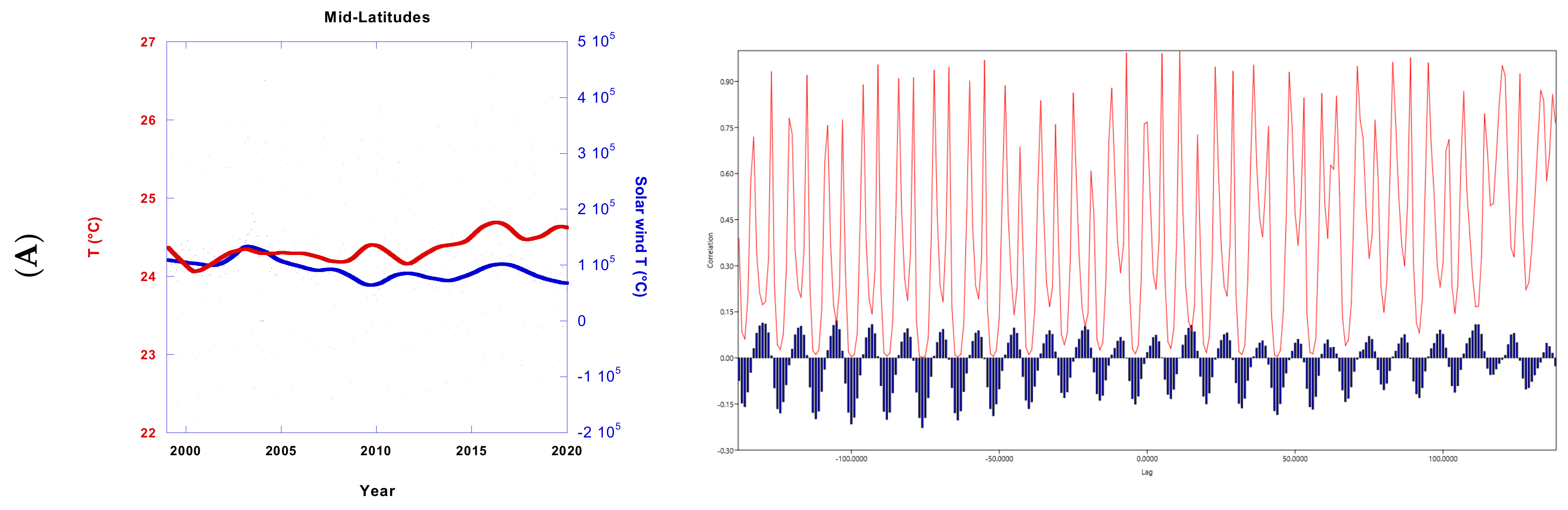
We plotted the time series of the two-meter temperature of the area located in the middle latitudes (in the range of 30° N to 60° N) with solar proton density at 1 AU and the scalar B-component of the solar wind at 1 AU obtained from the wind satellite (Figure 1), which is referred to as the primary interaction of the solar plasma with the outer geomagnetic field.

We found that there is a simultaneous and high correlation between the two-meter temperature of the atmosphere with the scalar B-component of the solar wind at 1 AU and solar protons during the period of the study. We can clearly see that the peaks and troughs of both curves are simultaneous. The correlation coefficient reaches about 0.9, as shown in the cross-correlation plot, for each cycle during our period of study, as shown in the right panels of Figure 1. In addition, we estimated Pearson’s correlation coefficient and examined the significance by a two-way t-test as shown in

Table 1. The correlation values by Pearson’s correlation and Tetrachoric statistic correlation [25] for solar wind.

Solar Wind Parameters	Two-Meter Temperature		t-Test (Two-Sample)
	Permutation p for Pearson’s Correlation	Tetrachoric (Statistic)	t:	p
Temperature	0.76	0.85018	42.674	2.6664−123
Proton Density	0.11	0.87175	181.13	2.9596−287
Scalar B	0.92	0.87175	177.72	5.1485−285

. This is because the solar wind has high temperatures, which heats the tropospheric air as an additional factor to the solar irradiance. This heating causes a few plasma particles in the troposphere, which interact with the Earth’s magnetic field lines.

This indicates that solar plasma that comes from the Sun and reaches the Earth causes a disturbance in the Earth’s magnetic field, as well as atmospheric temperature for mid-latitudes. The strong coherence with atmospheric temperature comes from solar protons and solar wind temperature. Simultaneously, with the solar wind, the scalar B-component becomes weaker. We found there was no correlation with other weather parameters.

The temperature oscillations that correlate to the impacts of the proton density are readily observable, as shown in Figure 1B. This indicates where the two-meter temperature fluctuation was greatest when the solar wind was strongest. This suggests that variations in solar wind activity are linked to variations in solar activity.

Our explanation of the correlation between atmospheric temperature and the B-scalar of the solar wind is that there is a dependence on the interplanetary magnetic field at 1 AU and solar wind parameters, which is associated with variations in its temperatures [11]. This coherence is shown in Figure 1C.

We examined these time series with the global value of the atmospheric temperature for northern and southern geospheres, and additionally to the low (0–30°) and high latitudes (60–90°) for both northern and southern geospheres. We found that the time series is clearer for mid-latitudes (30° N to 60° N).

It is noticeable that the density of protons strongly coincides with the temperature of the atmosphere. This is consistent with the results of [24], who found that variations in the altitudinal temperature profile observed during solar proton events are associated with a decrease in direct solar radiation at the Earth’s surface.

3.2. Weather Parameters-Dst Index Relationship

Pudovkin and Morozova [26] studied the effects of geomagnetic activity on the mesospheric electric fields. They used the Kp index. Their measurements show a clear dependence of the vertical electric fields on the geomagnetic activity at polar and high middle latitudes. They did not investigate the possible connection between the Kp index as an indication of geomagnetic activity and tropospheric weather parameters. Here, we use the Dst index to compare the synchronization between it and the tropospheric weather parameters.

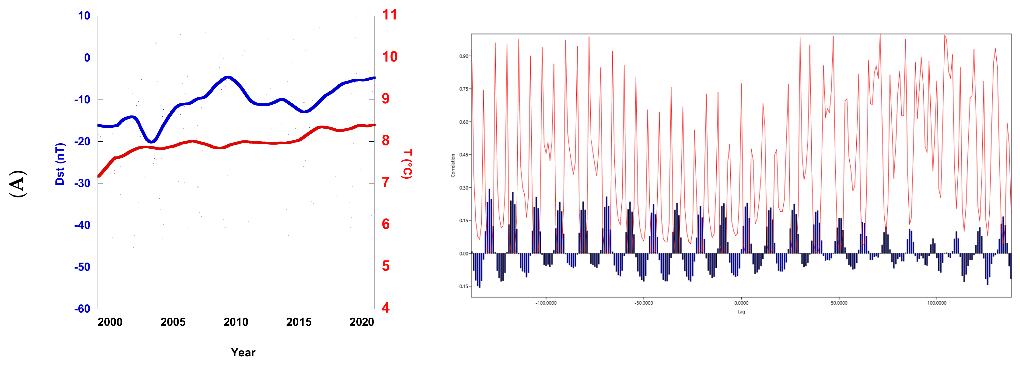
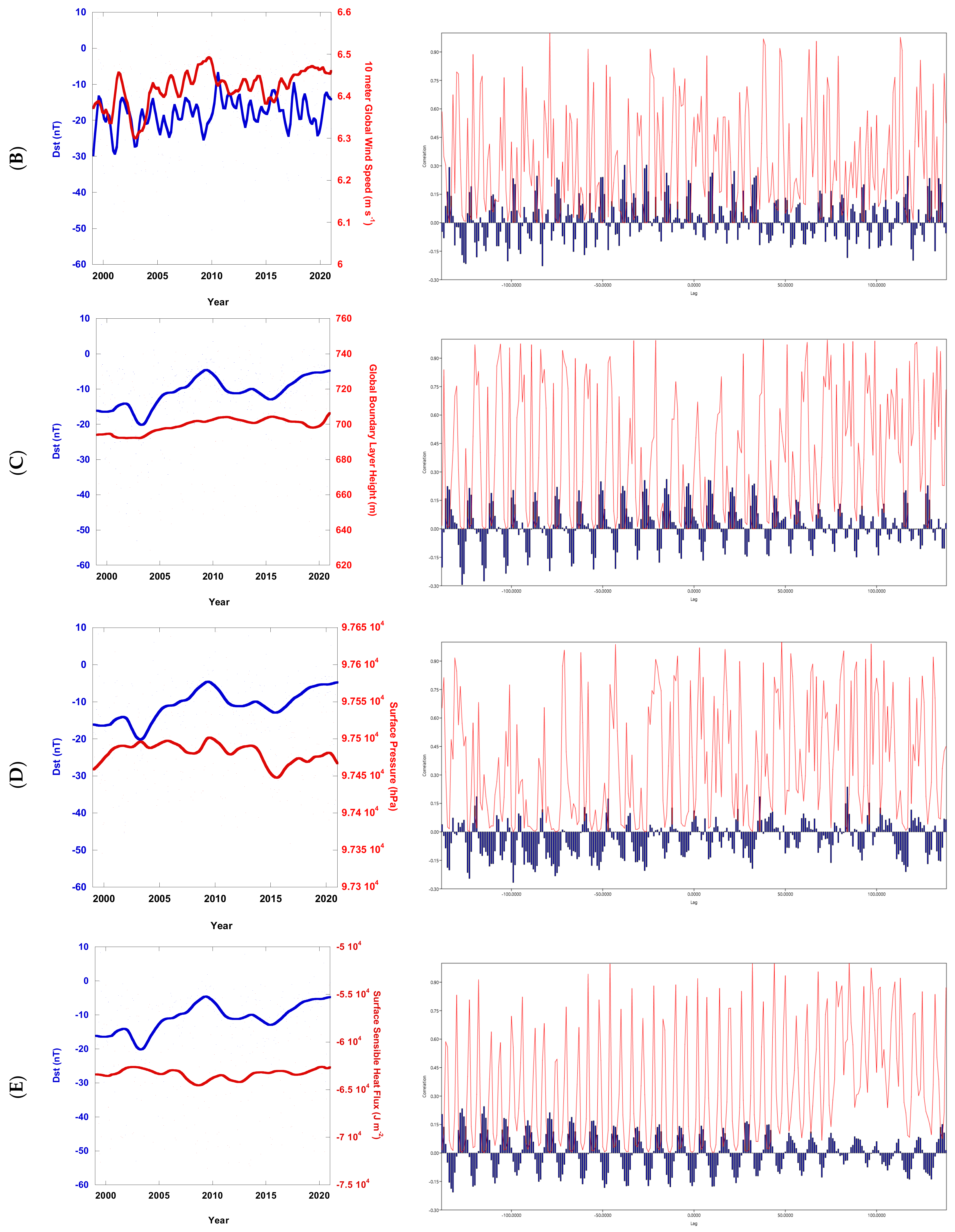
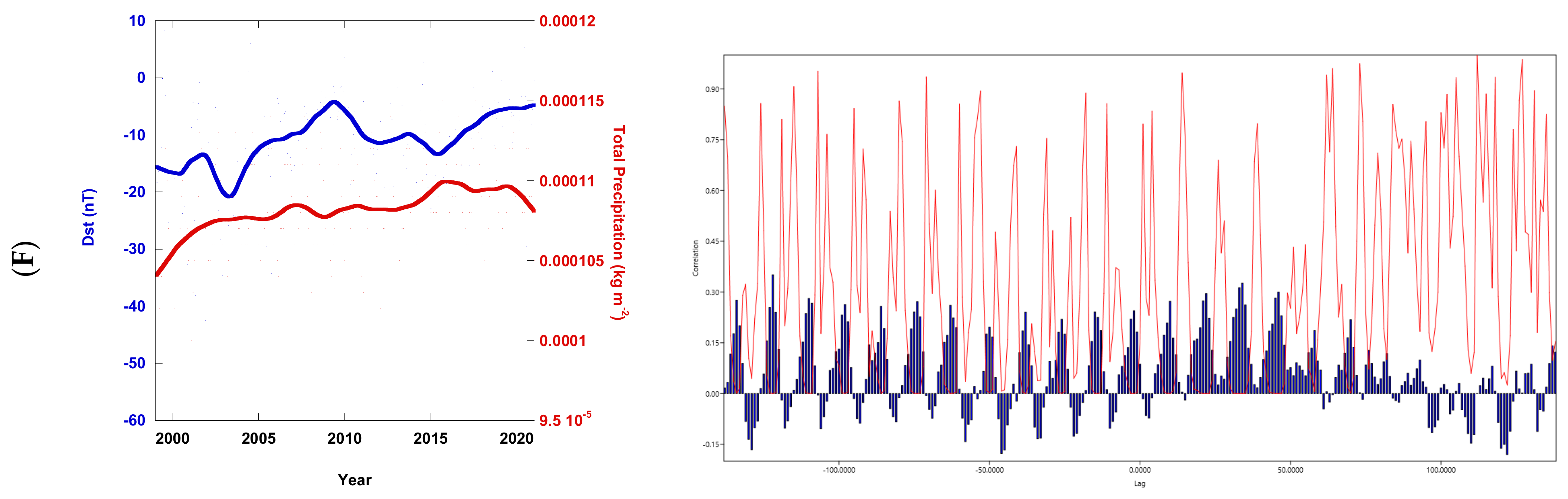
In Figure 2, we plotted the Dst index with all-weather parameters, two-meter temperature, global wind speed, global boundary layer height, surface pressure, surface sensible heat flux, and total precipitation.

We found there is a positive correlation of time series between Dst with global wind speed and surface pressure. In contrast, this time series gives a negative correlation with two-meter temperature, global boundary layer height, surface sensible heat flux, and total precipitation. The correlation coefficient reaches about 0.9, as shown in the cross-correlation plot, for each cycle during our period of study, as shown in the right panels of Figure 2. In addition, we estimated Pearson’s correlation coefficient and examined the significance by a two-way t-test as shown in

Table 2. Same as Table 1 but for Dst index.

Weather Parameters	Dst Index		t-Test (Two-Sample)
	Permutation p for Pearson’s Correlation	Tetrachoric (Statistic)	t:	p (Same Mean)
Temperature	0.7778	−0.60685	−63.683	1.2008−166
Global wind speed	0.5608	−0.60685	−31.923	1.7679−94
Global Boundary layer height	0.3014	0.96477	−382.71	0
Global surface pressure	0.0643	−0.60685	−29580	0
Surface Sensible heat flux	0.0102	0.73586	194.56	1.6472−83
Total Precipitation	0.1492	−0.60685	−20.584	1.2774−57

.

The strongest correlation comes with both time series Dst and global wind speed. which means that the horizontal geomagnetic field interacts with the atmospheric wind speeds and vice versa.

We noticed that the two-meter temperature has two variations. The main variation is the rising trend. This variation is equivalent to the rising with Dst. At the same time, the small variation comes with opposition.

This indicates that the change in the magnetic field affects atmospheric weather. Also, the weather influences the magnetic field.

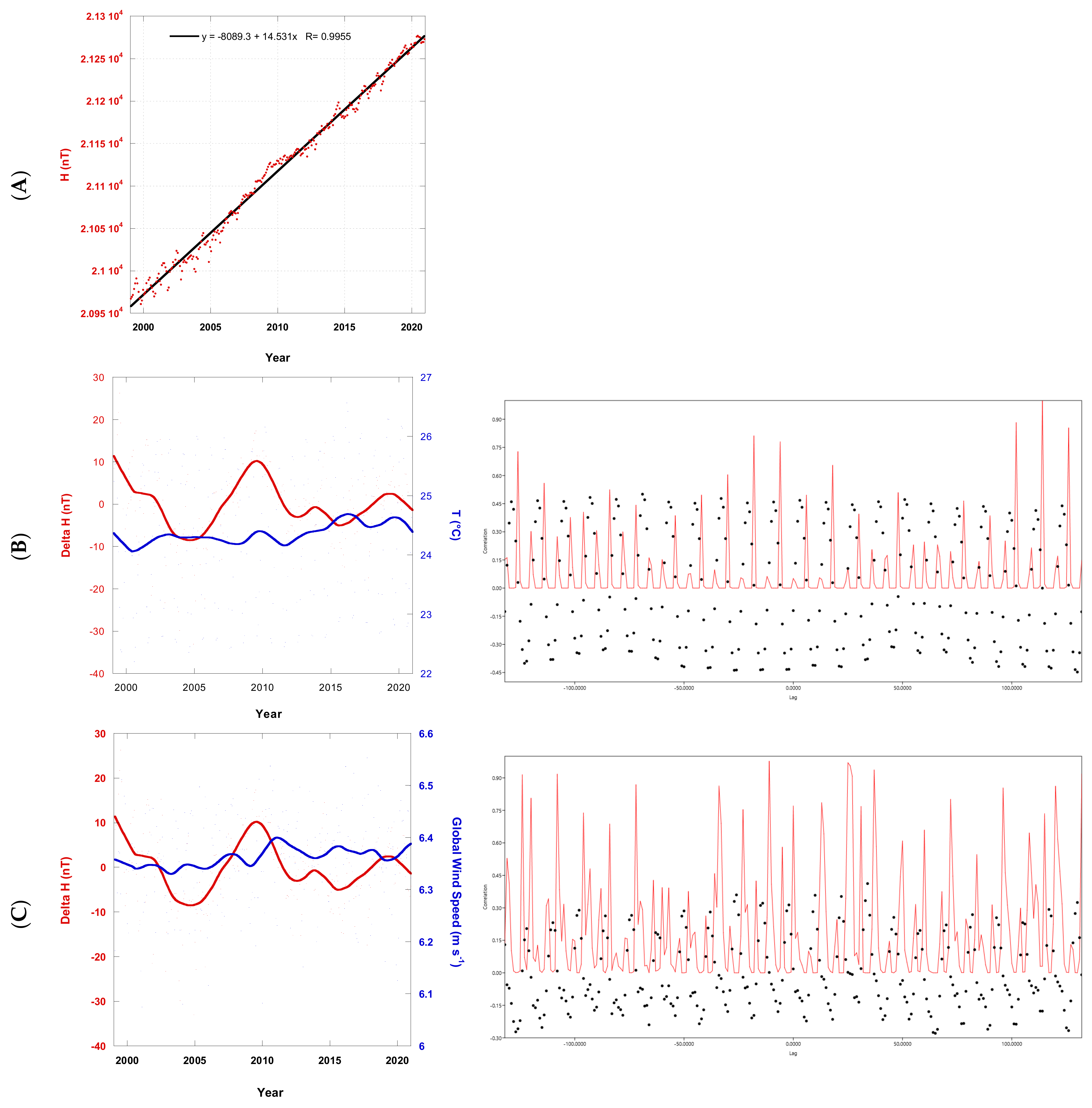
3.3. Weather-Earth’s Magnetic Field Strength

In Figure 3, we illustrate the time series of ΔH-component and two-meter temperature, global wind speed, global boundary layer height, surface pressure, total precipitation, and two-meter temperature at mid-latitudes (30° N–60° N).

The horizontal intensity of the geomagnetic field vector (H-component) rises with time during our study (1999–2021). During this period, there are small oscillations. The rising trend does not correlate with any weather parameters. But we need to examine the correlation with small oscillations only. Because of that, we want to deduce the smaller oscillations without a rising trend. Our solution is to derive the linear equation of the rising trend by fitting. Then, we use this equation to extract the small oscillations only (ΔH). ΔH gives the following:

ΔH = H − (−8089.3 + 14.531 × T)

where H is the H-component of the Earth’s magnetic field at the time T. The values are the linear fitting parameters, the intercept of H, and slope, respectively. These fitting parameters give a correlation coefficient equal to 0.9955.

We found that the small oscillations have strong coherence with weather parameters, as shown in Figure 3. The two-meter temperature and surface pressure give a positive correlation. Global wind speed, global boundary layer height, and total precipitation negatively correlate.

The correlation coefficient reaches about 0.9, as shown in the cross-correlation plot, for each cycle during our period of study, as shown in the right panels of Figure 3. In addition, we estimated Pearson’s correlation coefficient and examined the significance of two-way t-test as shown in

Table 3. Same as Table 1 but for ΔH-component.

Weather Parameters	ΔH-Component		t-Test (Two-Sample)
	Permutation p for Pearson’s Correlation	Tetrachoric (Statistic)	t:	p (Same Mean)
Temperature	0.05145	1	−44.703	6.9496−125
Global wind speed	0.77087	1	−12.604	8.2423−29
Global Boundary layer height	0.00012271	1	−389.77	0
Global surface pressure	0.00035516	1	−29309	0
Surface Sensible heat flux	3.7547 × 10−14	1	191.48	2.0531−284
Total Precipitation	0.27721	1	−0.86708	0.38669

. This result indicates that the magnetic field on the ground has two sources. The main source that is associated with the rising trend comes from the Earth’s core. The source of the small oscillations is atmospheric weather. This indicates that the weather has a slight effect on the Earth’s magnetic field at the Earth’s surface.

4. Discussion

It is obvious that the variability of climate change is dependent on solar activity, as manifested in the solar wind, and this variation can be significant. The change in two-meter temperature is consistent with the variation of the solar wind during the time series as a result of solar irradiance. The Earth’s surface temperature is affected by the variation of solar irradiance [27]. For example, after Earth’s surface absorption and reflection, irradiance can influence the temperature of the atmosphere. This variation depends on the change of distance from the Sun, the solar cycle, and cross-cycle fluctuations, all of which affect irradiance at the top of the atmosphere. On the other hand, this change in solar activity affects the geomagnetic field at the same time. The simultaneities between the two-meter temperature and the Dst index are shown in Figure 2A. This relationship does not mean the effect of the geomagnetic field at the Earth’s surface on atmospheric variables but means the simultaneous solar activity on both atmospheric variables and geomagnetic field effects only.

By studying the long-term temperature, ref. [16] discovered that there is a positive correlation between the Earth’s temperature with the magnetic field. This result agrees with our results during a shorter period of study. In addition, we found that it has a positive correlation with solar wind temperature. This means that the temperature of the solar wind reaching the Earth heats the atmosphere. We found that the Dst index gives a negative correlation with the tropospheric temperature.

The precipitation has a negative correlation with the Dst index. The H-component has two periodicities; the short one has a negative correlation but the long one has a positive correlation (during the period 1999–2021). This is consistent partially with the results of [18], as they discovered that there is a positive correlation between cloud cover and cosmic rays during the period 1980–1995. It is known that cosmic rays are linked to the heliomagnetic field, that is, they are affected by solar activity. Consequently, the Earth’s magnetic field is associated with those cosmic rays.

We note that the Dst has a strong association with global wind speed, as shown in Figure 2B and Figure 3B. This means that the variation in the geomagnetic disturbance moves the air in the troposphere. This indicates that the air contains a few charged particles that move according to the disturbances of the magnetic field. This conclusion is consistent with previous research findings that aerosols are associated with cosmic rays [16,18,19,20,21].

Observations and previous studies have shown that the altitude of the magnetosphere varies with time depending on solar activity as a result of the pressure of the solar wind on the magnetosphere [12]. In the current study, Figure 2C and Figure 3C show a variation in the boundary layer height synchronous with geomagnetic disturbances. In addition, Figure 2D and Figure 3D show a variation in the surface pressure too. This means that a change in the magnetic field is followed by the compression or rarefaction of air, especially containing some charged particles, which drives it to move. This is an additional force that leads to the wind’s movement. Although that force is weak compared to the known dynamic forces, these figures show that it has an important impact.

5. Conclusions

We studied the correlation between the atmospheric weather and geomagnetic strength during the period of 1999–2021. We found the strongest coherence comes with weather parameters of the mid-latitudes (30° N to 60° N) with the H-component.

In the outer magnetosphere, we found that there is a high coherence and simultaneity between the two-meter temperature with solar proton and solar wind temperature. Simultaneity with the solar wind scalar B-component comes weaker.

With the depths of the magnetosphere, we found that the Dst index has a strong correlation with all-weather parameters. A positive correlation was found between global wind speed and surface pressure. However, this gives a negative correlation with two-meter temperature, global boundary layer height, surface sensible heat flux, and total precipitation. The strongest correlation comes with both time series Dst and global wind speed.

We found that the atmospheric wind speeds causing variation in the strength of the magnetic field at the ground and the small oscillations in the magnetic field lead to variation in the speed of the wind and its directions. From this result, we conclude that the tropospheric air contains a little plasma particle which interacts with Earth’s magnetic field lines. This particle’s movement drags together with the natural air.

At the surface of the Earth, the variation of the magnetic field has two sources according to its large and small oscillations. We focus on small variations only because the main source of the large oscillations comes from the Earth’s core. We notice that the small oscillations in the magnetic field have strong coherence with the atmospheric weather. This indicates that the weather has a slight effect on the Earth’s magnetic field at the Earth’s surface.

Finally, there is a very strong correlation between atmospheric weather and the geomagnetic field. This relationship is lower at the Earth’s surface due to the strong influence of the source of the magnetic field coming from the center of the Earth. When we move towards the higher layers of the magnetosphere, the interaction between weather and the magnetic field strength is stronger. This indicates that space, especially the Sun, is the important external source of the variation in the atmospheric weather parameters.

References

- Hoyt, D.V.; Schatten, K.H.; Bering, E.A. The Role of the Sun in Climate Change. Phys. Today 1998, 51, 70. [Google Scholar] [CrossRef]
- Yousef, S.M. The solar Wolf-Gleissberg cycle and its influence on the Earth. In ICEHM2000; Cairo University: Giza, Egypt, 2000; pp. 267–293. [Google Scholar]
- Yousef, S. Expected cooling of the Earth and its implications on good security. Bull. L. Inst. Egypte Tom 2005, 80, 53–82. [Google Scholar]
- Zhao, J.; Han, Y.B.; Li, Z.A. The Effect of Solar Activity on the Annual Precipitation in the Beijing Area. Chin. J. Astron. Astrophys. 2004, 4, 189–197. Available online: http://www.solarstorms.org/Beijing.pdf (accessed on 1 March 2022). [CrossRef]
- Akasofu, S.-I. On the recovery from the Little Ice Age. Nat. Sci. 2010, 2, 1211–1224. [Google Scholar] [CrossRef]
- Yousef, S. Solar Induced Climate Changes on Millennium, Century and Solar Cycle scales. In Proceedings of the 4th IAGA Symposium, Hurghada, Egypt, 20–24 March 2016; Available online: http://iaga.cu.edu.eg/index.htm (accessed on 1 March 2022).
- Yousef, S.M. Solar Induced Climate Changes and Cooling of the Earth. In Modern Trends in Physics Research; World Scientific: Luxor, Egypt, 2011; pp. 296–308. [Google Scholar] [CrossRef]
- Mawad, R. On the correlation between Earth’s orbital perturbations and oscillations of sea level and concentration of greenhouse gases. J. Mod. Trends Phys. R. 2015, 15, 1–9. [Google Scholar] [CrossRef]
- Mawad, R. Coherence between sea level oscillations and orbital perturbations. Earth Space Sci. 2017, 4, 138–146. [Google Scholar] [CrossRef]
- Schmutz, W.K. Changes in the Total Solar Irradiance and climatic effects. J. Space Weather Space Clim. 2021, 11, 40. [Google Scholar] [CrossRef]
- Youssef, M.; Mahrous, A.; Mawad, R.; Ghamry, E.; Shaltout, M.; El-Nawawy, M.; Fahim, A. The effects of the solar magnetic polarity and the solar wind velocity on Bz-component of the interplanetary magnetic field. Adv. Space Res. 2012, 49, 1198–1202. [Google Scholar] [CrossRef]
- Mawad, R.; Youssef, M.; Yousef, S.; Abdel-Sattar, W. Quantizated variability of Earth’s magnetopause distance. J. Mod. Trends Phys. R. 2014, 14, 105–110. [Google Scholar] [CrossRef]
- King, J.W. Weather and the Earth’s magnetic field. Nature 1974, 247, 131–134. [Google Scholar] [CrossRef]
- King, J.W.; Willis, D.M. Magnetometeorology: Relationships between the Weather and Earth’s Magnetic Field. In Goddard Space Flight Center Possible Relationships between Solar Activity and Meteorol Phenomena; NASA: Merritt Island, FL, USA, 1975; pp. 39–41. [Google Scholar]
- Campuzano, S.A.; De Santis, A.; Pavon-Carrasco, F.J.; Osete, M.L.; Qamili, E. New perspectives in the study of the Earth’s magnetic field and climate connection: The use of transfer entropy. PLoS ONE 2018, 13, e0207270. [Google Scholar] [CrossRef]
- Lorenzen, B. Earth’s Magnetic Field—The Key to Global Warming. J. Geosci. Environ. Prot. 2019, 7, 25–38. [Google Scholar] [CrossRef]
- Bucha, V. Geomagnetic forcing of changes in climate and in the atmospheric circulation. J. Atmos. Sol. Terr. Phys. 1998, 60, 145–169. [Google Scholar] [CrossRef]
- Marsh, N. Cosmic Rays, Clouds, and Climate. Space Sci. Rev. 2000, 94, 215–230. [Google Scholar] [CrossRef]
- Shumilov, O.I.; Raspopov, O.M.; Kasatkina, E.A.; Turjansky, V.A.; Dergachev, V.A.; Prokhorov, N.S. Atmospheric Aerosols Created by Varying Cosmic Ray Activity—One of the Key Factors of Non-Direct Solar Forcing of Climate. Available online: https://articles.adsabs.harvard.edu/pdf/2000ESASP.463..543S (accessed on 1 March 2022).
- Usoskin, I.G.; Kovaltsov, G.A. Cosmic rays and climate of the Earth: Possible connection. Comptes Rendus Geosci. 2008, 340, 441–450. [Google Scholar] [CrossRef]
- Kitaba, I.; Hyodo, M.; Katoh, S.; Dettman, D.L.; Sato, H. Midlatitude cooling caused by geomagnetic field minimum during polarity reversal. Proc. Natl. Acad. Sci. USA 2013, 110, 1215–1220. [Google Scholar] [CrossRef]
- Kilifarska, N.; Bakhmutov, V.; Melnyk, G. Coupling between Geomagnetic Field and Earth’s Climate System; Essa, K.S., Mahmoud, K.H., Eds.; IntechOpen: London, UK, 2022; Working Title “Magnetosphere”. [Google Scholar] [CrossRef]
- Lyatsky, W.; Tan, A.; Lyatskaya, S. Effect of Solar magnetic field polarity on interplanetary magnetic field Bz. Geophys. Res. Lett. 2003, 30, 2258. [Google Scholar] [CrossRef]
- Pudovkin, M.; Morozova, A. Time variation of atmospheric pressure and circulation associated with temperature changes during Solar Proton Events. J. Atmos. Sol. Terr. Phys. 1998, 60, 1729–1737. [Google Scholar] [CrossRef]
- El-Hashash, E.F.; El-Absy, K.M. Methods for Determining the Tetrachoric Correlation Coefficient for Binary Variables. Asian J. Probab. Stat. 2018, 2, 1–12. [Google Scholar] [CrossRef]
- Zadorozhny, A.M.; Tyutin, A.A. Effects of geomagnetic activity on the mesospheric electric fields. Ann. Geophys. Eur. Geosci. Union 1998, 16, 1544–1551. [Google Scholar] [CrossRef]
- Lawin, A.E.; Niyongendako, M.; Manirakiza, C. Solar Irradiance and Temperature Variability and Projected Trends Analysis in Burundi. Climate 2019, 7, 83. [Google Scholar] [CrossRef]