How Inflationary Gravitons Affect the Force of Gravity

Abstract

We employ an unregulated computation of the graviton self-energy from gravitons on the de Sitter background to infer the renormalized result. This is used to quantum-correct the linearized Einstein equation. We solve this equation for the potentials that represent the gravitational response to a static, point mass. We find large spatial and temporal logarithmic corrections to the Newtonian potential and to the gravitational shift. Although suppressed by a minuscule loop-counting parameter, these corrections cause perturbation theory to break down at large distances and late times. Another interesting fact is that gravitons induce up to three large logarithms, whereas a loop of massless, minimally coupled scalars produces only a single large logarithm. This is in line with corrections to the graviton mode function: a loop of gravitons induces two large logarithms, whereas a scalar loop gives none.

1. Introduction

A key prediction of primordial inflation is that virtual gravitons of a cosmological scale are ripped out of the vacuum [1,2]. The occupation number for each wave vector $\overrightarrow{k}$ is staggering:

$$N(\eta ,k)=\frac{\pi {\mathrm{\Delta }}_h^2\left(k\right)}{64G{k}^2}\times a^2\left(\eta \right),$$

(1)

where ${\mathrm{\Delta }}_h^2\left(k\right)$ is the tensor power spectrum, G is Newton’s constant, and $a\left(\eta \right)$ is the scale factor at conformal time $\eta$. Our goal is to study how these gravitons change the force of gravity.

We can describe the background geometry of cosmology in conformal coordinates:

$$d{s}^2=a^2\left(\eta \right)\left[-d{\eta }^2+d\overrightarrow{x}·d\overrightarrow{x}\right]⟹H\equiv \frac{a^{\prime }}{a^2},ϵ\equiv -\frac{H^{\prime }}{a{H}^2},$$

(2)

where $H\left(\eta \right)$ is the Hubble parameter and $ϵ\left(\eta \right)$ is the first slow roll parameter. A reasonable paradigm for inflation is provided by the special case of de Sitter ($ϵ=0$, constant H, and $a\left(\eta \right)=-1/H\eta$), which is tempting because there are analytic expressions for the graviton propagator [3,4] and because there is no mixing between gravitons and the matter fields that drive inflation [5,6]. One quantum-corrects the linearized Einstein equation using the graviton self-energy $-i\left[{}^{\mu \nu }{\Sigma }^{\rho \sigma }\right](x;x^{\prime })$, which is the 1PI (one-particle irreducible) two-graviton function,

$${\mathcal{D}}^{\mu \nu \rho \sigma }{h}_{\rho \sigma }\left(x\right)-\int d^4{x}^{\prime }\left[{}^{\mu \nu }{\Sigma }^{\rho \sigma }\right](x;x^{\prime })h_{\rho \sigma }\left(x^{\prime }\right)=\frac{1}{2}\kappa T_{\mathrm{lin}}^{\mu \nu }\left(x\right).$$

(3)

Here, ${\kappa }^2\equiv 16\pi G$ is the loop-counting parameter, $h_{\mu \nu }\equiv (g_{\mu \nu }-a^2{\eta }_{\mu \nu })/\kappa$ is the graviton field, $T_{\mathrm{lin}}^{\mu \nu }\left(x\right)$ is the linearized stress tensor, and ${\mathcal{D}}^{\mu \nu \rho \sigma }$ is the graviton kinetic operator in the same gauge that was used to compute $-i\left[{}^{\mu \nu }{\Sigma }^{\rho \sigma }\right](x;x^{\prime })$. Our two aims in this work are (1) to infer a fully renormalized result for $-i\left[{}^{\mu \nu }{\Sigma }^{\rho \sigma }\right](x;x^{\prime })$ at one loop from an old computation [7] that was made without regularization and (2) to work out one-loop corrections to the gravitational response to a point mass.

There are four sections to this paper, of which this Introduction is the first. Section 2 describes our procedure for extracting the renormalized self-energy from the unregulated result, with technical details consigned to an Appendix A. Section 3 solves (3) for one-loop corrections to the gravitational potentials induced by a point mass. Our conclusions comprise Section 4.

2. Quantum Linearized Einstein Equation

This section derives an explicit expression for the quantum-corrected Einstein Equation (3). Our first tasks are specifying the gauge-fixed kinetic operator ${\mathcal{D}}^{\mu \nu \rho \sigma }$, explaining how we represent the tensor structure of the graviton self-energy, and giving $3+1$ decompositions of both. The main part of this section describes the process through which we infer most of the renormalized, Schwinger–Keldysh result for the graviton self-energy from an unregulated, noncoincident computation [7]. At the section’s end, we give a direct, dimensionally regulated computation of the local four-point contribution, and we discuss the need for a fully dimensionally regulated calculation.

2.1. 3 + 1 Decomposition

In the simplest gauge and $D=3+1$ dimensions, the gauge-fixed kinetic operator takes the form [3,4]:

$${\mathcal{D}}^{\mu \nu \rho \sigma }=\frac{1}{2}{\eta }^{\mu (\rho }{\eta }^{\sigma )\nu }{D}_A-\frac{1}{4}{\eta }^{\mu \nu }{\eta }^{\rho \sigma }{D}_A+2a^4{H}^2{\delta }_0^{(\mu }{\eta }^{\nu \left)\right(\rho }{\delta }_0^{\sigma )}.$$

(4)

Here, $D_A$ is the massless, minimally coupled scalar kinetic operator:

$$D_A=-a^2\left[{\partial }_0^2+2aH{\partial }_0-{\nabla }^2\right]={\partial }^{\mu }{a}^2{\partial }_{\mu }.$$

(5)

The $3+1$ decomposition of ${\mathcal{D}}^{\mu \nu \rho \sigma }{h}_{\rho \sigma }$ is

$$\begin{array}{ccc}\hfill {\mathcal{D}}^{00\rho \sigma }{h}_{\rho \sigma }& =& \frac{1}{4}{D}_A(h_{00}+h_{kk})-2a^4{H}^2{h}_{00},\hfill \end{array}$$

(6)

$$\begin{array}{ccc}\hfill {\mathcal{D}}^{0i\rho \sigma }{h}_{\rho \sigma }& =& -\frac{1}{2}{D}_B{h}_{0i},\hfill \end{array}$$

(7)

$$\begin{array}{ccc}\hfill {\mathcal{D}}^{ij\rho \sigma }{h}_{\rho \sigma }& =& \frac{1}{2}{D}_A\left[h_{ij}+\frac{1}{2}{\delta }_{ij}(h_{00}-h_{kk})\right],\hfill \end{array}$$

(8)

where $D_B$ stands for the kinetic operator of a massless, conformally coupled scalar:

$$D_B=-a^2\left[{\partial }_0^2+2aH{\partial }_0-{\nabla }^2+2a^2{H}^2\right]=a{\partial }^{2}a.$$

(9)

Note that adding (6) and the trace of (8) gives a relation for $h_{00}$,

$$\left({\mathcal{D}}^{00\rho \sigma }+{\mathcal{D}}^{kk\rho \sigma }\right)h_{\rho \sigma }=D_B{h}_{00}.$$

(10)

Using general tensor analysis on a general cosmological background (2), we can represent the graviton self-energy as the sum of 21 tensor differential operators $\left[{}^{\mu \nu }{\mathcal{D}}^{\rho \sigma }\right]$ acting on scalar functions of $\eta$, ${\eta }^{\prime }$, and $\parallel \overrightarrow{x}-{\overrightarrow{x}}^{\prime }\parallel$ [8],

$$-i\left[{}^{\mu \nu }{\Sigma }^{\rho \sigma }\right](x;x^{\prime })=\sum _{i=1}^{21}\left[{}^{\mu \nu }{\mathcal{D}}_i^{\rho \sigma }\right]\times T^i(x;x^{\prime }).$$

(11)

The 21 basis tensors are constructed from ${\delta }_0^{\mu }$, the spatial part of the Minkowski metric ${\overline{\eta }}^{\mu \nu }\equiv {\eta }^{\mu \nu }+{\delta }_0^{\mu }{\delta }_0^{\nu }$, and the spatial derivative operator ${\overline{\partial }}^{\mu }\equiv {\partial }^{\mu }+{\delta }_0^{\mu }{\partial }_0$. These 21 tensors are listed in

Table 1. The 21 basis tensors used in Expression (11). The pairs $(3,4)$, $(5,6)$, $(7,8)$, $(10,11)$, $(14,15)$, $(16,17)$, and $(19,20)$ are related by reflection.

i	$\left[{}^{\mathit{\mu }\mathit{\nu }}{\mathcal{D}}_{\mathit{i}}^{\mathit{\rho }\mathit{\sigma }}\right]$	i	$\left[{}^{\mathit{\mu }\mathit{\nu }}{\mathcal{D}}_{\mathit{i}}^{\mathit{\rho }\mathit{\sigma }}\right]$	i	$\left[{}^{\mathit{\mu }\mathit{\nu }}{\mathcal{D}}_{\mathit{i}}^{\mathit{\rho }\mathit{\sigma }}\right]$
1	${\overline{\eta }}^{\mu \nu }{\overline{\eta }}^{\rho \sigma }$	8	${\overline{\partial }}^{\mu }{\overline{\partial }}^{\nu }{\overline{\eta }}^{\rho \sigma }$	15	${\delta }_0^{(\mu }{\overline{\partial }}^{\nu )}{\delta }_0^{\rho }{\delta }_0^{\sigma }$
2	${\overline{\eta }}^{\mu (\rho }{\overline{\eta }}^{\sigma )\nu }$	9	${\delta }_0^{(\mu }{\overline{\eta }}^{\nu \left)\right(\rho }{\delta }_0^{\sigma )}$	16	${\delta }_0^{\mu }{\delta }_0^{\nu }{\overline{\partial }}^{\rho }{\overline{\partial }}^{\sigma }$
3	${\overline{\eta }}^{\mu \nu }{\delta }_0^{\rho }{\delta }_0^{\sigma }$	10	${\delta }_0^{(\mu }{\overline{\eta }}^{\nu \left)\right(\rho }{\overline{\partial }}^{\sigma )}$	17	${\overline{\partial }}^{\mu }{\overline{\partial }}^{\nu }{\delta }_0^{\rho }{\delta }_0^{\sigma }$
4	${\delta }_0^{\mu }{\delta }_0^{\nu }{\overline{\eta }}^{\rho \sigma }$	11	${\overline{\partial }}^{(\mu }{\overline{\eta }}^{\nu \left)\right(\rho }{\delta }_0^{\sigma )}$	18	${\delta }_0^{(\mu }{\overline{\partial }}^{\nu )}{\delta }_0^{(\rho }{\overline{\partial }}^{\sigma )}$
5	${\overline{\eta }}^{\mu \nu }{\delta }_0^{(\rho }{\overline{\partial }}^{\sigma )}$	12	${\overline{\partial }}^{(\mu }{\overline{\eta }}^{\nu \left)\right(\rho }{\overline{\partial }}^{\sigma )}$	19	${\delta }_0^{(\mu }{\overline{\partial }}^{\nu )}{\overline{\partial }}^{\rho }{\overline{\partial }}^{\sigma }$
6	${\delta }_0^{(\mu }{\overline{\partial }}^{\nu )}{\overline{\eta }}^{\rho \sigma }$	13	${\delta }_0^{\mu }{\delta }_0^{\nu }{\delta }_0^{\rho }{\delta }_0^{\sigma }$	20	${\overline{\partial }}^{\mu }{\overline{\partial }}^{\nu }{\delta }_0^{(\rho }{\overline{\partial }}^{\sigma )}$
7	${\overline{\eta }}^{\mu \nu }{\overline{\partial }}^{\rho }{\overline{\partial }}^{\sigma }$	14	${\delta }_0^{\mu }{\delta }_0^{\nu }{\delta }_0^{(\rho }{\overline{\partial }}^{\sigma )}$	21	${\overline{\partial }}^{\mu }{\overline{\partial }}^{\nu }{\overline{\partial }}^{\rho }{\overline{\partial }}^{\sigma }$

.

Table 2. Scalar coefficient functions in Expression (11), which are related by reflection.

i	Relation	i	Relation
$3,4$	$T^4(x;x^{\prime })=+T^3(x^{\prime };x)$	$14,15$	$T^{15}(x;x^{\prime })=-T^{14}(x^{\prime };x)$
$5,6$	$T^6(x;x^{\prime })=-T^5(x^{\prime };x)$	$16,17$	$T^{17}(x;x^{\prime })=+T^{16}(x^{\prime };x)$
$7,8$	$T^8(x;x^{\prime })=+T^7(x^{\prime };x)$	$19,20$	$T^{20}(x;x^{\prime })=-T^{19}(x^{\prime };x)$
$10,11$	$T^{11}(x;x^{\prime })=-T^{10}(x^{\prime };x)$

gives the 7 pairs of $T^i(x;x^{\prime })$, which are related by reflection invariance, $-i\left[{}^{\mu \nu }{\Sigma }^{\rho \sigma }\right](x;x^{\prime })=-i\left[{}^{\rho \sigma }{\Sigma }^{\mu \nu }\right](x^{\prime };x)$.

The $3+1$ decomposition of $\left[{}^{\mu \nu }{\Sigma }^{\rho \sigma }\right](x;x^{\prime })h_{\rho \sigma }\left(x^{\prime }\right)$ is

$$\begin{array}{c}\hfill {\displaystyle \left[{}^{00}{\Sigma }^{\rho \sigma }\right]h_{\rho \sigma }⟶i{T}^4{h}_{kk}+i{T}^{13}{h}_{00}+i{T}^{14}{h}_{0k,k}+i{T}^{16}{h}_{k\ell ,k\ell },}\\ \hfill {\displaystyle \left[{}^{0i}{\Sigma }^{\rho \sigma }\right]h_{\rho \sigma }⟶\frac{i}{2}{\partial }_i\left[T^6{h}_{kk}+T^{15}{h}_{00}+T^{18}{h}_{0k,k}+T^{19}{h}_{k\ell ,k\ell }\right]}\end{array}$$

(12)

$$\begin{array}{cc}& +\frac{i}{2}{T}^9{h}_{0i}+\frac{i}{2}{T}^{10}{h}_{ik,k},\hfill \\ \hfill {\displaystyle \left[{}^{ij}{\Sigma }^{\rho \sigma }\right]h_{\rho \sigma }⟶i{\delta }_{ij}\left[T^1{h}_{kk}+T^3{h}_{00}+T^5{h}_{0k,k}+T^7{h}_{k\ell ,k\ell }\right]+i{T}^2{h}_{ij}}\end{array}$$

(13)

$$\begin{array}{ccc}& & +i{\partial }_{(i}\left[T^{11}{h}_{j)0}+T^{12}{h}_{j)k,k}\right]+i{\partial }_i{\partial }_j\left[T^8{h}_{kk}+T^{17}{h}_{00}+T^{20}{h}_{0k,k}+T^{21}{h}_{k\ell ,k\ell }\right].\hfill \end{array}$$

(14)

Some of these relations were simplified using transition invariance to partially integrate spatial derivatives from the coefficient functions $T^i(x;x^{\prime })$ onto the graviton field.

2.2. The Quantum Correction

Suppose that $S\left[g\right]$ stands for the classical action, with ghost and gauge fixing action $S_g[h,\overline{\theta },\theta ]$ and counterterms $\mathrm{\Delta }S\left[g\right]$. We can give an analytic expression for the one-loop graviton self-energy using an expectation value of variations of these actions:

$$\begin{array}{c}\hfill {\displaystyle -i\left[{}^{\mu \nu }{\Sigma }^{\rho \sigma }\right](x;x^{\prime })=\langle \mathrm{\Omega }\left|T^{*}\right[{\left[\frac{i\delta S\left[g\right]}{\delta h_{\mu \nu }\left(x\right)}\right]}_{hh}{\left[\frac{i\delta S\left[g\right]}{\delta h_{\rho \sigma }\left(x^{\prime }\right)}\right]}_{hh}+{\left[\frac{i\delta S\left[g\right]}{\delta h_{\mu \nu }\left(x\right)}\right]}_{\overline{\theta }\theta }}\\ \times {\left[\frac{i\delta S\left[g\right]}{\delta h_{\rho \sigma }\left(x^{\prime }\right)}\right]}_{\overline{\theta }\theta }+{\left[\frac{i{\delta }^{2}S\left[g\right]}{\delta h_{\mu \nu }\left(x\right)\delta h_{\rho \sigma }\left(x^{\prime }\right)}\right]}_{hh}+{\left[\frac{i{\delta }^2\mathrm{\Delta }S\left[g\right]}{\delta h_{\mu \nu }\left(x\right)\delta h_{\rho \sigma }\left(x^{\prime }\right)}\right]}_1\left]\right|\mathrm{\Omega }\rangle .\hfill \end{array}$$

(15)

The $T^{*}$-ordering symbol indicates that derivatives are taken outside the time ordering symbol, and the various subscripts give the number of weak fields that contribute. The analogous Feynman diagrams are shown in Figure 1.

2.2.1. The $D=4$ Result

The unregulated result [7] can best be understood by considering how a dimensionally regulated computation of $-i\left[{}^{\mu \nu }{\Sigma }^{\rho \sigma }\right](x;x^{\prime })$ would look. The general forms of the three-graviton and four-graviton vertices are [3,9]:1

$$\begin{array}{ccc}\hfill \kappa a^{D-2}h\partial h\partial h& ,& \kappa H{a}^{D-1}hh\partial h,\hfill \end{array}$$

(16)

$$\begin{array}{ccc}\hfill {\kappa }^2{a}^{D-2}hh\partial h\partial h& ,& {\kappa }^{2}H{a}^{D-1}hhh\partial h.\hfill \end{array}$$

(17)

There is a plethora of different index contractions, but contributions to the first two (nonlocal) diagrams of Figure 1 take the general form:

$$\kappa a^{D-2}\times \partial {\partial }^{\prime }i\mathrm{\Delta }(x;x^{\prime })\times \partial {\partial }^{\prime }i\mathrm{\Delta }(x;x^{\prime })\times \kappa {a^{\prime }}^{D-2},$$

(18)

with $i\mathrm{\Delta }(x;x^{\prime })$ standing for a ghost or graviton propagator and the understanding that one derivative at each vertex could be replaced by a factor of H times the appropriate scale factor. Note also that, when an external leg happens to be differentiated, then minus the derivative acts on everything. On the other hand, the third (four-point) diagram of Figure 1 is local:

$${\kappa }^2{a}^{D-2}\times \partial {\partial }^{\prime }i\mathrm{\Delta }(x;x^{\prime })\times i{\delta }^D(x-x^{\prime }),$$

(19)

with the same understanding concerning derivatives. The last (counterterm) diagram of Figure 1 is also local:

$$\frac{{\kappa }^2{a}^{D-4}}{D-4}\times {\partial }^2{{\partial }^{\prime }}^2\times i{\delta }^D(x-x^{\prime }),$$

(20)

with the stipulation that any number of the four derivatives could each be replaced by a factor of $Ha$.

The gauge for this computation was fixed by adding [3,4]

$${\mathcal{L}}_{GF}=-\frac{a^{D-2}}{2}{\eta }^{\mu \nu }{F}_{\mu }{F}_{\nu },F_{\mu }={\eta }^{\rho \sigma }\left(h_{\mu \rho ,\sigma }-\frac{1}{2}{h}_{\rho \sigma ,\mu }+(D-2)aH{h}_{\mu \rho }{\delta }_{\sigma }^0\right).$$

(21)

In this gauge, the ghost and graviton propagators become sums of constant tensor factors multiplied by simple scalar propagators:

$$\begin{array}{ccc}\hfill i\left[{}_{\mu }{\mathrm{\Delta }}_{\rho }\right](x;x^{\prime })& =& {\overline{\eta }}_{\mu \rho }\times i{\mathrm{\Delta }}_A(x;x^{\prime })-{\delta }_{\mu }^0{\delta }_{\nu }^0\times i{\mathrm{\Delta }}_B(x;x^{\prime }),\hfill \end{array}$$

(22)

$$\begin{array}{ccc}\hfill i\left[{}_{\mu \nu }{\mathrm{\Delta }}_{\rho \sigma }\right](x;x^{\prime })& =& \sum _{I=A,B,C}\left[{}_{\mu \nu }{T}_{\rho \sigma }^I\right]\times i{\mathrm{\Delta }}_I(x;x^{\prime }).\hfill \end{array}$$

(23)

The various $\left[{}_{\mu \nu }{T}_{\rho \sigma }^I\right]$ are

$$\begin{array}{c}\hfill \left[{}_{\mu \nu }{T}_{\rho \sigma }^A\right]=2{\overline{\eta }}_{\mu (\rho }{\overline{\eta }}_{\sigma )\nu }-\frac{2}{D-3}{\overline{\eta }}_{\mu \nu }{\overline{\eta }}_{\rho \sigma },\left[{}_{\mu \nu }{T}_{\rho \sigma }^B\right]=-4{\delta }_{(\mu }^0{\overline{\eta }}_{\nu \left)\right(\rho }{\delta }_{\sigma )}^0,\end{array}$$

(24)

$$\begin{array}{c}\hfill \left[{}_{\mu \nu }{T}_{\rho \sigma }^C\right]=\frac{2E_{\mu \nu }{E}_{\rho \sigma }}{(D-2)(D-3)},E_{\mu \nu }\equiv (D-3){\delta }_{\mu }^0{\delta }_{\nu }^0+{\overline{\eta }}_{\mu \nu }.\end{array}$$

(25)

Most of the scalar propagators can be expressed using a function $A\left(y\right)$ of the de Sitter length function $y(x;x^{\prime })\equiv a{a}^{\prime }{H}^2\mathrm{\Delta }{x}^2$:

$$\begin{array}{ccc}\hfill i{\mathrm{\Delta }}_A(x;x^{\prime })& =& A\left(y\right)+kln\left(a{a}^{\prime }\right)k\equiv \frac{H^{D-2}}{{\left(4\pi \right)}^{\frac{D}{2}}}\frac{\mathrm{\Gamma }(D-1)}{\mathrm{\Gamma }\left(\frac{D}{2}\right)},\hfill \end{array}$$

(26)

$$\begin{array}{ccc}\hfill i{\mathrm{\Delta }}_B(x;x^{\prime })& =& B\left(y\right)\equiv -\frac{[(4y-y^2)A^{\prime }\left(y\right)+(2-y)k]}{2(D-2)},\hfill \end{array}$$

(27)

$$\begin{array}{ccc}\hfill i{\mathrm{\Delta }}_C(x;x^{\prime })& =& C\left(y\right)\equiv \frac{1}{2}(2-y)B\left(y\right)+\frac{k}{D-3}.\hfill \end{array}$$

(28)

The first derivative of $A\left(y\right)$ is [10,11]

$$\begin{array}{c}{\displaystyle A^{\prime }\left(y\right)=-\frac{H^{D-2}}{4{\left(4\pi \right)}^{\frac{D}{2}}}\{\mathrm{\Gamma }\left(\frac{D}{2}\right){\left(\frac{4}{y}\right)}^{\frac{D}{2}}+\mathrm{\Gamma }\left(\frac{D}{2}+1\right){\left(\frac{4}{y}\right)}^{\frac{D}{2}-1}}\hfill \\ \hfill +\sum _{n=0}^{\infty }\left[\frac{\mathrm{\Gamma }(n+\frac{D}{2}+2)}{\mathrm{\Gamma }(n+3)}{\left(\frac{y}{4}\right)}^{n-\frac{D}{2}+2}-\frac{\mathrm{\Gamma }(n+D)}{\mathrm{\Gamma }(n+\frac{D}{2}+1)}{\left(\frac{y}{4}\right)}^n\right]\}.\end{array}$$

(29)

Note that the $y^n$ and $y^{n-\frac{D}{2}-2}$ terms cancel for $D=4$, so they only contribute when multiplied by a sufficiently singular term.

Divergences occur in the effective field Equation (3) when the integration over ${x^{\prime }}^{\mu }$ carries it to coincidence, ${x^{\prime }}^{\mu }=x^{\mu }$. Hence, the first two (nonlocal) diagrams of Figure 1 can be taken to $D=4$ away from coincidence, which also makes the two local diagrams vanish. This was performed for the unregulated computation [7]. That computation was tractable because taking $D=4$ simplifies the propagators,

$$\begin{array}{ccc}\hfill i\left[{}_{\mu }{\mathrm{\Delta }}_{\rho }^{D=4}\right](x;x^{\prime })& =& \frac{1}{4{\pi }^2}\left\{\frac{{\eta }_{\mu \rho }}{a{a}^{\prime }\mathrm{\Delta }{x}^2}-\frac{1}{2}{H}^{2}ln\left(H^2\mathrm{\Delta }{x}^2\right){\overline{\eta }}_{\mu \rho }\right\},\hfill \\ \hfill i\left[{}_{\mu \nu }{\mathrm{\Delta }}_{\rho \sigma }^{D=4}\right](x;x^{\prime })& =& \frac{1}{4{\pi }^2}\{\frac{(2{\eta }_{\mu (\rho }{\eta }_{\sigma )\nu }-{\eta }_{\mu \nu }{\eta }_{\rho \sigma })}{a{a}^{\prime }\mathrm{\Delta }{x}^2}\hfill \end{array}$$

(30)

$$\begin{array}{ccc}& & -H^{2}ln\left(H^2\mathrm{\Delta }{x}^2\right)\left({\overline{\eta }}_{\mu (\rho }{\overline{\eta }}_{\sigma )\nu }-{\overline{\eta }}_{\mu \nu }{\overline{\eta }}_{\rho \sigma }\right)\}.\hfill \end{array}$$

(31)

Because one of the propagators in the nonlocal diagrams (18) might not carry any derivatives, the coefficient functions $T^i(x;x^{\prime })$ in our representation (11) of the graviton self-energy take the form:

$$T^i(x;x^{\prime })\equiv T_N^i(x;x^{\prime })+T_L^i(x;x^{\prime })\times ln\left(H^2\mathrm{\Delta }{x}^2\right).$$

(32)

The coefficient functions $T_L^i(x;x^{\prime })$ are given in

Table 3. Each tabulated term must be multiplied by $-\frac{{\kappa }^2}{64{\pi }^4}$.

i	Coefficient Functions ${\mathit{T}}_{\mathit{L}}^{\mathit{i}}(\mathit{x};{\mathit{x}}^{\prime })$ in Expression (32)
1	$8a^2{a^{\prime }}^2{H}^4\times [\frac{4\mathrm{\Delta }{\eta }^2}{\mathrm{\Delta }{x}^6}+\frac{1}{\mathrm{\Delta }{x}^4}]+4a^3{a^{\prime }}^3{H}^6\times [\frac{4\mathrm{\Delta }{\eta }^4}{\mathrm{\Delta }{x}^6}-\frac{\mathrm{\Delta }{\eta }^2}{\mathrm{\Delta }{x}^4}+\frac{3}{\mathrm{\Delta }{x}^2}]$
2	$-16a^2{a^{\prime }}^2{H}^4\times [\frac{4\mathrm{\Delta }{\eta }^2}{\mathrm{\Delta }{x}^6}+\frac{1}{\mathrm{\Delta }{x}^4}]-4a^3{a^{\prime }}^3{H}^6\times [\frac{8\mathrm{\Delta }{\eta }^4}{\mathrm{\Delta }{x}^6}+\frac{1}{\mathrm{\Delta }{x}^2}]$
3	$8a^3{a^{\prime }}^3{H}^6\times [\frac{\mathrm{\Delta }{\eta }^2}{\mathrm{\Delta }{x}^4}-\frac{2}{\mathrm{\Delta }{x}^2}]-4a^3{a^{\prime }}^2{H}^5\times [\frac{4\mathrm{\Delta }{\eta }^3}{\mathrm{\Delta }{x}^6}-\frac{\mathrm{\Delta }\eta }{\mathrm{\Delta }{x}^4}]$
5	$16a^2{a^{\prime }}^2{H}^4\times \frac{\mathrm{\Delta }\eta }{\mathrm{\Delta }{x}^4}+4a^3{a^{\prime }}^2{H}^5\times [\frac{2\mathrm{\Delta }{\eta }^2}{\mathrm{\Delta }{x}^4}+\frac{3}{\mathrm{\Delta }{x}^2}]$
7	$-8a^2{a^{\prime }}^2{H}^4\times \frac{1}{\mathrm{\Delta }{x}^2}-2a^3{a^{\prime }}^3{H}^6\times \frac{\mathrm{\Delta }{\eta }^2}{\mathrm{\Delta }{x}^2}-2a^3{a^{\prime }}^2{H}^5\times \frac{\mathrm{\Delta }\eta }{\mathrm{\Delta }{x}^2}$
9	$-96a{a}^{\prime }{H}^2\times [\frac{16\mathrm{\Delta }{\eta }^4}{\mathrm{\Delta }{x}^{10}}+\frac{12\mathrm{\Delta }{\eta }^2}{\mathrm{\Delta }{x}^8}+\frac{1}{\mathrm{\Delta }{x}^6}]-4a^2{a^{\prime }}^2{H}^4\times [\frac{24\mathrm{\Delta }{\eta }^4}{\mathrm{\Delta }{x}^8}+\frac{8\mathrm{\Delta }{\eta }^2}{\mathrm{\Delta }{x}^6}-\frac{1}{\mathrm{\Delta }{x}^4}]$
10	$96a{a}^{\prime }{H}^2\times [\frac{2\mathrm{\Delta }{\eta }^3}{\mathrm{\Delta }{x}^8}+\frac{\mathrm{\Delta }\eta }{\mathrm{\Delta }{x}^6}]+12a^2{a^{\prime }}^2{H}^4\times [\frac{4\mathrm{\Delta }{\eta }^3}{\mathrm{\Delta }{x}^6}+\frac{\mathrm{\Delta }\eta }{\mathrm{\Delta }{x}^4}]+a^3{a^{\prime }}^3{H}^6\times [\frac{8\mathrm{\Delta }{\eta }^3}{\mathrm{\Delta }{x}^4}-\frac{4\mathrm{\Delta }\eta }{\mathrm{\Delta }{x}^2}]$
	$-8a^2{a}^{\prime }{H}^3\times [\frac{4\mathrm{\Delta }{\eta }^2}{\mathrm{\Delta }{x}^6}+\frac{1}{\mathrm{\Delta }{x}^4}]-4a^3{a}^{\prime 2}{H}^5\times [\frac{2\mathrm{\Delta }{\eta }^2}{\mathrm{\Delta }{x}^4}-\frac{1}{\mathrm{\Delta }{x}^2}]$
12	$-8a{a}^{\prime }{H}^2\times [\frac{4\mathrm{\Delta }{\eta }^2}{\mathrm{\Delta }{x}^6}+\frac{1}{\mathrm{\Delta }{x}^4}]-2a^2{a^{\prime }}^2{H}^4\times [\frac{6\mathrm{\Delta }{\eta }^2}{\mathrm{\Delta }{x}^4}-\frac{9}{\mathrm{\Delta }{x}^2}]+4a^3{a^{\prime }}^3{H}^6\times \frac{\mathrm{\Delta }{\eta }^2}{\mathrm{\Delta }{x}^2}$
13	$-96a{a}^{\prime }{H}^2\times [\frac{16\mathrm{\Delta }{\eta }^4}{\mathrm{\Delta }{x}^{10}}+\frac{12\mathrm{\Delta }{\eta }^2}{\mathrm{\Delta }{x}^8}+\frac{1}{\mathrm{\Delta }{x}^6}]+4a^2{a^{\prime }}^2{H}^4\times [\frac{24\mathrm{\Delta }{\eta }^4}{\mathrm{\Delta }{x}^8}+\frac{56\mathrm{\Delta }{\eta }^2}{\mathrm{\Delta }{x}^6}+\frac{11}{\mathrm{\Delta }{x}^4}]$
	$+8a^3{a^{\prime }}^3{H}^6\times [\frac{4\mathrm{\Delta }{\eta }^4}{\mathrm{\Delta }{x}^6}-\frac{2\mathrm{\Delta }{\eta }^2}{\mathrm{\Delta }{x}^4}+\frac{3}{\mathrm{\Delta }{x}^2}]$
14	$192a{a}^{\prime }{H}^2\times [\frac{2\mathrm{\Delta }{\eta }^3}{\mathrm{\Delta }{x}^8}+\frac{\mathrm{\Delta }\eta }{\mathrm{\Delta }{x}^6}]+8a^2{a^{\prime }}^2{H}^4\times [\frac{4\mathrm{\Delta }{\eta }^3}{\mathrm{\Delta }{x}^6}-\frac{3\mathrm{\Delta }\eta }{\mathrm{\Delta }{x}^4}]$
	$-16a^2{a}^{\prime }{H}^3\times [\frac{4\mathrm{\Delta }{\eta }^2}{\mathrm{\Delta }{x}^6}+\frac{1}{\mathrm{\Delta }{x}^4}]-16a^3{a^{\prime }}^2{H}^5\times [\frac{\mathrm{\Delta }{\eta }^2}{\mathrm{\Delta }{x}^4}+\frac{1}{\mathrm{\Delta }{x}^2}]$
16	$-8a{a}^{\prime }{H}^2\times [\frac{4\mathrm{\Delta }{\eta }^2}{\mathrm{\Delta }{x}^6}+\frac{1}{\mathrm{\Delta }{x}^4}]+2a^2{a^{\prime }}^2{H}^4\times [-\frac{6\mathrm{\Delta }{\eta }^2}{\mathrm{\Delta }{x}^4}+\frac{1}{\mathrm{\Delta }{x}^2}]-2a^3{a^{\prime }}^3{H}^6\times \frac{\mathrm{\Delta }{\eta }^2}{\mathrm{\Delta }{x}^2}$
	$+16a^2{a}^{\prime }{H}^3\times \frac{\mathrm{\Delta }\eta }{\mathrm{\Delta }{x}^4}+6a^3{a^{\prime }}^2{H}^5\times \frac{\mathrm{\Delta }\eta }{\mathrm{\Delta }{x}^2}$
18	$-24a{a}^{\prime }{H}^2\times [\frac{4\mathrm{\Delta }{\eta }^2}{\mathrm{\Delta }{x}^6}+\frac{1}{\mathrm{\Delta }{x}^4}]-2a^2{a^{\prime }}^2{H}^4\times [\frac{6\mathrm{\Delta }{\eta }^2}{\mathrm{\Delta }{x}^4}+\frac{5}{\mathrm{\Delta }{x}^2}]$
19	$8a{a}^{\prime }{H}^2\times \frac{\mathrm{\Delta }\eta }{\mathrm{\Delta }{x}^4}+6a^2{a^{\prime }}^2{H}^4\times \frac{\mathrm{\Delta }\eta }{\mathrm{\Delta }{x}^2}-4a^2{a}^{\prime }{H}^3\times \frac{1}{\mathrm{\Delta }{x}^2}$

and the $T_N^i(x;x^{\prime })$ are given in

Table 4. Each of the tabulated terms must be multiplied by $-\frac{{\kappa }^2}{64{\pi }^4}$.

i	Coefficient Functions ${\mathit{T}}_{\mathit{N}}^{\mathit{i}}(\mathit{x};{\mathit{x}}^{\prime })$ in Expression (32)
1	$\frac{\frac{736}{5}}{\mathrm{\Delta }{x}^8}-a{a}^{\prime }{H}^2[\frac{616\mathrm{\Delta }{\eta }^2}{\mathrm{\Delta }{x}^8}+\frac{\frac{220}{3}}{\mathrm{\Delta }{x}^6}]-a^2{a^{\prime }}^2{H}^4[\frac{96\mathrm{\Delta }{\eta }^4}{\mathrm{\Delta }{x}^8}+\frac{\frac{812}{3}\mathrm{\Delta }{\eta }^2}{\mathrm{\Delta }{x}^6}+\frac{19}{\mathrm{\Delta }{x}^4}]-a^3{a^{\prime }}^3{H}^6[\frac{64\mathrm{\Delta }{\eta }^4}{\mathrm{\Delta }{x}^6}+\frac{22\mathrm{\Delta }{\eta }^2}{\mathrm{\Delta }{x}^4}]$
2	$\frac{\frac{1952}{5}}{\mathrm{\Delta }{x}^8}-a{a}^{\prime }{H}^2[\frac{416\mathrm{\Delta }{\eta }^2}{\mathrm{\Delta }{x}^8}+\frac{\frac{128}{3}}{\mathrm{\Delta }{x}^6}]-a^2{a^{\prime }}^2{H}^4[\frac{\frac{112}{3}\mathrm{\Delta }{\eta }^2}{\mathrm{\Delta }{x}^6}-\frac{56}{\mathrm{\Delta }{x}^4}]+a^3{a^{\prime }}^3{H}^6[\frac{32\mathrm{\Delta }{\eta }^4}{\mathrm{\Delta }{x}^6}+\frac{12\mathrm{\Delta }{\eta }^2}{\mathrm{\Delta }{x}^4}]$
	$-184[\frac{\frac{8}{5}\mathrm{\Delta }{\eta }^2}{\mathrm{\Delta }{x}^{10}}+\frac{1}{\mathrm{\Delta }{x}^8}]+32a{a}^{\prime }{H}^2[\frac{36\mathrm{\Delta }{\eta }^4}{\mathrm{\Delta }{x}^{10}}+\frac{14\mathrm{\Delta }{\eta }^2}{\mathrm{\Delta }{x}^8}-\frac{\frac{43}{3}}{\mathrm{\Delta }{x}^6}]$
3	$-a^2{a^{\prime }}^2{H}^4[\frac{288\mathrm{\Delta }{\eta }^4}{\mathrm{\Delta }{x}^8}-\frac{\frac{1228}{3}\mathrm{\Delta }{\eta }^2}{\mathrm{\Delta }{x}^6}+\frac{145}{\mathrm{\Delta }{x}^4}]+4a^3{a^{\prime }}^3{H}^6[\frac{16\mathrm{\Delta }{\eta }^4}{\mathrm{\Delta }{x}^6}+\frac{5\mathrm{\Delta }{\eta }^2}{\mathrm{\Delta }{x}^4}]$
	$-8aH[\frac{232\mathrm{\Delta }{\eta }^3}{\mathrm{\Delta }{x}^{10}}+\frac{203\mathrm{\Delta }\eta }{\mathrm{\Delta }{x}^8}]+4a^2{a}^{\prime }{H}^3[\frac{74\mathrm{\Delta }{\eta }^3}{\mathrm{\Delta }{x}^8}-\frac{\frac{319}{3}\mathrm{\Delta }\eta }{\mathrm{\Delta }{x}^6}]-a^3{a^{\prime }}^2{H}^5\times \frac{38\mathrm{\Delta }\eta }{\mathrm{\Delta }{x}^4}$
5	$\frac{\frac{368}{5}\mathrm{\Delta }\eta }{\mathrm{\Delta }{x}^8}-32a{a}^{\prime }{H}^2[\frac{9\mathrm{\Delta }{\eta }^3}{\mathrm{\Delta }{x}^8}-\frac{\frac{4}{3}\mathrm{\Delta }\eta }{\mathrm{\Delta }{x}^6}]+4a^2{a^{\prime }}^2{H}^4[\frac{8\mathrm{\Delta }{\eta }^3}{\mathrm{\Delta }{x}^6}-\frac{\mathrm{\Delta }\eta }{\mathrm{\Delta }{x}^4}]$
	$+232aH[\frac{2\mathrm{\Delta }{\eta }^2}{\mathrm{\Delta }{x}^8}+\frac{1}{\mathrm{\Delta }{x}^6}]-2a^2{a}^{\prime }{H}^3[\frac{\frac{28}{3}\mathrm{\Delta }{\eta }^2}{\mathrm{\Delta }{x}^6}-\frac{23}{\mathrm{\Delta }{x}^4}]-a^3{a^{\prime }}^2{H}^5\times \frac{12\mathrm{\Delta }{\eta }^2}{\mathrm{\Delta }{x}^4}$
7	$-\frac{\frac{92}{15}}{\mathrm{\Delta }{x}^6}+a{a}^{\prime }{H}^2[\frac{24\mathrm{\Delta }{\eta }^2}{\mathrm{\Delta }{x}^6}+\frac{\frac{7}{3}}{\mathrm{\Delta }{x}^4}]+a^2{a^{\prime }}^2{H}^4[\frac{8\mathrm{\Delta }{\eta }^2}{\mathrm{\Delta }{x}^4}-\frac{3}{\mathrm{\Delta }{x}^2}]+a^3{a^{\prime }}^3{H}^6\times \frac{\mathrm{\Delta }{\eta }^2}{\mathrm{\Delta }{x}^2}$
	$-aH\times \frac{\frac{116}{3}\mathrm{\Delta }\eta }{\mathrm{\Delta }{x}^6}-a^2{a}^{\prime }{H}^3\times \frac{\frac{23}{3}\mathrm{\Delta }\eta }{\mathrm{\Delta }{x}^4}+a^3{a^{\prime }}^2{H}^5\times \frac{\mathrm{\Delta }\eta }{\mathrm{\Delta }{x}^2}$
9	$-16[\frac{\frac{488}{5}\mathrm{\Delta }{\eta }^2}{\mathrm{\Delta }{x}^{10}}+\frac{61}{\mathrm{\Delta }{x}^8}]+16a{a}^{\prime }{H}^2[\frac{88\mathrm{\Delta }{\eta }^4}{\mathrm{\Delta }{x}^{10}}-\frac{10\mathrm{\Delta }{\eta }^2}{\mathrm{\Delta }{x}^8}-\frac{35}{\mathrm{\Delta }{x}^6}]+4a^2{a^{\prime }}^2{H}^4[\frac{8\mathrm{\Delta }{\eta }^4}{\mathrm{\Delta }{x}^8}+\frac{2\mathrm{\Delta }{\eta }^2}{\mathrm{\Delta }{x}^6}-\frac{3}{\mathrm{\Delta }{x}^4}]$
10	$\frac{\frac{976}{5}\mathrm{\Delta }\eta }{\mathrm{\Delta }{x}^8}-16a{a}^{\prime }{H}^2[\frac{8\mathrm{\Delta }{\eta }^3}{\mathrm{\Delta }{x}^8}-\frac{\frac{23}{3}\mathrm{\Delta }\eta }{\mathrm{\Delta }{x}^6}]-2a^2{a^{\prime }}^2{H}^4[\frac{\frac{16}{3}\mathrm{\Delta }{\eta }^3}{\mathrm{\Delta }{x}^6}-\frac{23\mathrm{\Delta }\eta }{\mathrm{\Delta }{x}^4}]$
	$+a^3{a^{\prime }}^3{H}^6\times \frac{4\mathrm{\Delta }{\eta }^3}{\mathrm{\Delta }{x}^4}+aH\times \frac{\frac{64}{3}}{\mathrm{\Delta }{x}^6}+8a^2{a}^{\prime }{H}^3[\frac{\frac{4}{3}\mathrm{\Delta }{\eta }^2}{\mathrm{\Delta }{x}^6}-\frac{5}{\mathrm{\Delta }{x}^4}]-a^3{a^{\prime }}^2{H}^5\times \frac{4\mathrm{\Delta }{\eta }^2}{\mathrm{\Delta }{x}^4}$
12	$-\frac{\frac{488}{15}}{\mathrm{\Delta }{x}^6}+\frac{32}{3}a{a}^{\prime }{H}^2[\frac{\mathrm{\Delta }{\eta }^2}{\mathrm{\Delta }{x}^6}-\frac{1}{\mathrm{\Delta }{x}^4}]-a^2{a^{\prime }}^2{H}^4[\frac{\frac{10}{3}\mathrm{\Delta }{\eta }^2}{\mathrm{\Delta }{x}^4}-\frac{8}{\mathrm{\Delta }{x}^2}]-a^3{a^{\prime }}^3{H}^6\times \frac{2\mathrm{\Delta }{\eta }^2}{\mathrm{\Delta }{x}^2}$
13	$16[\frac{336\mathrm{\Delta }{\eta }^4}{\mathrm{\Delta }{x}^{12}}+\frac{336\mathrm{\Delta }{\eta }^2}{\mathrm{\Delta }{x}^{10}}+\frac{63}{\mathrm{\Delta }{x}^8}]+4a{a}^{\prime }{H}^2[\frac{336\mathrm{\Delta }{\eta }^4}{\mathrm{\Delta }{x}^{10}}+\frac{868\mathrm{\Delta }{\eta }^2}{\mathrm{\Delta }{x}^8}+\frac{409}{\mathrm{\Delta }{x}^6}]$
	$+a^2{a^{\prime }}^2{H}^4[\frac{424\mathrm{\Delta }{\eta }^4}{\mathrm{\Delta }{x}^8}+\frac{144\mathrm{\Delta }{\eta }^2}{\mathrm{\Delta }{x}^6}+\frac{557}{\mathrm{\Delta }{x}^4}]-24a^3{a^{\prime }}^3{H}^6[\frac{4\mathrm{\Delta }{\eta }^4}{\mathrm{\Delta }{x}^6}-\frac{\mathrm{\Delta }{\eta }^2}{\mathrm{\Delta }{x}^4}]$
14	$-672[\frac{\frac{8}{5}\mathrm{\Delta }{\eta }^3}{\mathrm{\Delta }{x}^{10}}+\frac{\mathrm{\Delta }\eta }{\mathrm{\Delta }{x}^8}]-8a{a}^{\prime }{H}^2[\frac{30\mathrm{\Delta }{\eta }^3}{\mathrm{\Delta }{x}^8}+\frac{\frac{107}{3}\mathrm{\Delta }\eta }{\mathrm{\Delta }{x}^6}]-4a^2{a^{\prime }}^2{H}^4[\frac{16\mathrm{\Delta }{\eta }^3}{\mathrm{\Delta }{x}^6}-\frac{7\mathrm{\Delta }\eta }{\mathrm{\Delta }{x}^4}]$
	$-16aH[\frac{4\mathrm{\Delta }{\eta }^2}{\mathrm{\Delta }{x}^8}+\frac{\frac{35}{3}}{\mathrm{\Delta }{x}^6}]-2a^2{a}^{\prime }{H}^3[\frac{\frac{68}{3}\mathrm{\Delta }{\eta }^2}{\mathrm{\Delta }{x}^6}+\frac{137}{\mathrm{\Delta }{x}^4}]+a^3{a^{\prime }}^2{H}^5\times \frac{16\mathrm{\Delta }{\eta }^2}{\mathrm{\Delta }{x}^4}$
16	$4[\frac{\frac{84}{5}\mathrm{\Delta }{\eta }^2}{\mathrm{\Delta }{x}^8}+\frac{\frac{13}{3}}{\mathrm{\Delta }{x}^6}]+a{a}^{\prime }{H}^2[\frac{24\mathrm{\Delta }{\eta }^2}{\mathrm{\Delta }{x}^6}+\frac{\frac{127}{3}}{\mathrm{\Delta }{x}^4}]+a^2{a^{\prime }}^2{H}^4[\frac{6\mathrm{\Delta }{\eta }^2}{\mathrm{\Delta }{x}^4}+\frac{5}{\mathrm{\Delta }{x}^2}]$
	$-a^3{a^{\prime }}^3{H}^6\times \frac{3\mathrm{\Delta }{\eta }^2}{\mathrm{\Delta }{x}^2}-aH\times \frac{28\mathrm{\Delta }\eta }{\mathrm{\Delta }{x}^6}+a^2{a}^{\prime }{H}^3\times \frac{\frac{49}{3}\mathrm{\Delta }\eta }{\mathrm{\Delta }{x}^4}+a^3{a^{\prime }}^2{H}^5\times \frac{\mathrm{\Delta }\eta }{\mathrm{\Delta }{x}^2}$
18	$8[\frac{\frac{168}{5}\mathrm{\Delta }{\eta }^2}{\mathrm{\Delta }{x}^8}+\frac{\frac{29}{3}}{\mathrm{\Delta }{x}^6}]+4a{a}^{\prime }{H}^2[\frac{12\mathrm{\Delta }{\eta }^2}{\mathrm{\Delta }{x}^6}-\frac{23}{\mathrm{\Delta }{x}^4}]+a^2{a^{\prime }}^2{H}^4\times \frac{10\mathrm{\Delta }{\eta }^2}{\mathrm{\Delta }{x}^4}$
19	$-\frac{\frac{112}{5}\mathrm{\Delta }\eta }{\mathrm{\Delta }{x}^6}-8a{a}^{\prime }{H}^2\times \frac{\mathrm{\Delta }\eta }{\mathrm{\Delta }{x}^4}-a^2{a^{\prime }}^2{H}^4\times \frac{\mathrm{\Delta }\eta }{\mathrm{\Delta }{x}^2}+aH\times \frac{\frac{50}{3}}{\mathrm{\Delta }{x}^4}$
21	$\frac{\frac{14}{5}}{\mathrm{\Delta }{x}^4}$

. Both are functions of a, $a^{\prime }$, $\mathrm{\Delta }\eta \equiv \eta -{\eta }^{\prime }$ and inverse powers of the Poincaré interval $\mathrm{\Delta }{x}^2\equiv \parallel \overrightarrow{x}-{\overrightarrow{x}}^{\prime }{\parallel }^2-\left(\right|\eta -{\eta }^{\prime }{|-i\epsilon )}^2$.

2.2.2. Recovering the Renormalized Result

In [12], we presented a four-step procedure for reconstructing the dimensionally regulated result for the first two diagrams of Figure 1:

1.

Express each $T_L^i(x;x^{\prime })$ as a sum of derivatives acting on three integrable functions:

$$\frac{1}{\mathrm{\Delta }{x}^2},\frac{\mathrm{\Delta }\eta }{\mathrm{\Delta }{x}^2},\frac{\mathrm{\Delta }{\eta }^2}{\mathrm{\Delta }{x}^2};$$

(33)

2.

Commute the various derivatives to the left of the multiplicative factor of $ln\left(H^2\mathrm{\Delta }{x}^2\right)$;

3.

Write the sum of the remainder $\mathrm{\Delta }{T}_L^i(x;x^{\prime })$ from Step 2 and $T_N^i(x;x^{\prime })$ as the sum of derivatives acting on the same integrable functions (33) and $1/\mathrm{\Delta }{x}^4$;

4.

Recognize the factors of $1/\mathrm{\Delta }{x}^4$ from Step 3 as the $D=4$ limit of $1/\mathrm{\Delta }{x}^{2D-4}$, and isolate the ultraviolet divergences on delta functions, which can be absorbed into counterterms.

Below, we explain the rationale for each step and provide details. We also implement the various steps on $T^{12}(x;x^{\prime })$:

$$\begin{array}{c}\hfill {\displaystyle T_L^{12}(x;x^{\prime })=-\frac{{\kappa }^{2}ln\left(H^2\mathrm{\Delta }{x}^2\right)}{64{\pi }^4}\{a{a}^{\prime }{H}^2\left[-\frac{32\mathrm{\Delta }{\eta }^2}{\mathrm{\Delta }{x}^6}-\frac{8}{\mathrm{\Delta }{x}^4}\right]}\end{array}$$

$$\begin{array}{c}+a^2{a^{\prime }}^2{H}^4\left[-\frac{12\mathrm{\Delta }{\eta }^2}{\mathrm{\Delta }{x}^4}+\frac{18}{\mathrm{\Delta }{x}^2}\right]+a^3{a^{\prime }}^3{H}^6\left[\frac{4\mathrm{\Delta }{\eta }^2}{\mathrm{\Delta }{x}^2}\right]\},\hfill \end{array}$$

(34)

$$T_N^{12}(x;x^{\prime })=-\frac{{\kappa }^2}{64{\pi }^4}\{-\frac{\frac{488}{15}}{\mathrm{\Delta }{x}^6}+a{a}^{\prime }H\left[\frac{\frac{32}{3}\mathrm{\Delta }{\eta }^2}{\mathrm{\Delta }{x}^6}-\frac{\frac{32}{3}}{\mathrm{\Delta }{x}^6}\right]$$

$$\begin{array}{ccc}& & +a^2{a^{\prime }}^2{H}^4\left[-\frac{\frac{10}{3}\mathrm{\Delta }{\eta }^2}{\mathrm{\Delta }{x}^4}+\frac{8}{\mathrm{\Delta }{x}^2}\right]+a^3{a^{\prime }}^3{H}^6\left[-\frac{2\mathrm{\Delta }{\eta }^4}{\mathrm{\Delta }{x}^2}\right]\}.\hfill \end{array}$$

(35)

To understand the rationale behind Step 1, note that a single factor of $ln\left(H^2\mathrm{\Delta }{x}^2\right)$ from the propagators (30) and (31) can only contribute to one of the $T_L^i(x;x^{\prime })$ if no derivatives act on one of the two propagators in (18). In that case, all of the derivatives must act on the other propagator, and it is this differentiated propagator, multiplied by the scale factors from the vertices, that appears in $T_L^i(x;x^{\prime })$. It follows that we can express $T_L^i(x;x^{\prime })$ as the sum of products of scale factors multiplied by derivatives of the three integrable functions (33). For example, $T_L^{12}(x;x^{\prime })$ in Expression (34) can be written as

$$\begin{array}{c}{\displaystyle T_L^{12}(x;x^{\prime })=-\frac{{\kappa }^{2}ln\left(H^2\mathrm{\Delta }{x}^2\right)}{64{\pi }^4}\{a{a}^{\prime }{H}^2\times -4{\partial }_0^2\left(\frac{1}{\mathrm{\Delta }{x}^2}\right)}\hfill \\ \hfill +a^2{a^{\prime }}^2{H}^4\left[-6{\partial }_0\left(\frac{\mathrm{\Delta }\eta }{\mathrm{\Delta }{x}^2}\right)+\frac{24}{\mathrm{\Delta }{x}^2}\right]+a^3{a^{\prime }}^3{H}^6\left[\frac{4\mathrm{\Delta }{\eta }^2}{\mathrm{\Delta }{x}^2}\right]\}.\end{array}$$

(36)

Appendix A contains a number of useful identities (A2)–(A11) for extracting derivatives.

Step 2 consists of commuting the multiplicative factor of $ln\left(H^2\mathrm{\Delta }{x}^2\right)$ through the derivatives to multiply the three integrable functions (33). Of course, this produces a “remainder” $\mathrm{\Delta }{T}_L^i(x;x^{\prime })$ in which derivatives act on the logarithm to produce a term like those in $T_N^i(x;x^{\prime })$. For example, carrying out Step 2 on Expression (36) for $T_L^{12}(x;x^{\prime })$ gives

$$\begin{array}{c}{\displaystyle T_L^{12}(x;x^{\prime })=-\frac{{\kappa }^2}{64{\pi }^4}\{a{a}^{\prime }{H}^2\times -4{\partial }_0^2\left(\frac{ln\left(H^2\mathrm{\Delta }{x}^2\right)}{\mathrm{\Delta }{x}^2}\right)+a^2{a^{\prime }}^2{H}^4[-6{\partial }_0}\hfill \\ \times \left(\frac{\mathrm{\Delta }\eta ln\left(H^2\mathrm{\Delta }{x}^2\right)}{\mathrm{\Delta }{x}^2}\right)+\frac{24ln\left(H^2\mathrm{\Delta }{x}^2\right)}{\mathrm{\Delta }{x}^2}]+a^3{a^{\prime }}^3{H}^6\times \frac{4\mathrm{\Delta }{\eta }^{2}ln\left(H^2\mathrm{\Delta }{x}^2\right)}{\mathrm{\Delta }{x}^2}\}\hfill \\ \hfill -\frac{{\kappa }^2}{64{\pi }^4}\left\{a{a}^{\prime }{H}^2\left[-\frac{48\mathrm{\Delta }{\eta }^2}{\mathrm{\Delta }{x}^6}-\frac{8}{\mathrm{\Delta }{x}^4}\right]+a^2{a^{\prime }}^2{H}^4\times -\frac{12\mathrm{\Delta }{\eta }^4}{\mathrm{\Delta }{x}^6}\right\}.\end{array}$$

(37)

Identities (A12)–(A20) in Appendix A facilitate these reductions. It is useful at this stage to identify six integrable functions, with a factor of $2\pi i$ extracted for future convenience,

$$\begin{array}{ccc}\hfill 2\pi i{A}_1\equiv \frac{ln\left(H^2\mathrm{\Delta }{x}^2\right)}{\mathrm{\Delta }{x}^2}& ,& 2\pi i{A}_2\equiv \frac{1}{\mathrm{\Delta }{x}^2},\hfill \end{array}$$

(38)

$$\begin{array}{ccc}\hfill 2\pi i{B}_1\equiv \frac{\mathrm{\Delta }\eta ln\left(H^2\mathrm{\Delta }{x}^2\right)}{\mathrm{\Delta }{x}^2}& ,& 2\pi i{B}_2\equiv \frac{\mathrm{\Delta }\eta }{\mathrm{\Delta }{x}^2},\hfill \end{array}$$

(39)

$$\begin{array}{ccc}\hfill 2\pi i{C}_1\equiv \frac{\mathrm{\Delta }{\eta }^{2}ln\left(H^2\mathrm{\Delta }{x}^2\right)}{\mathrm{\Delta }{x}^2}& ,& 2\pi i{C}_2\equiv \frac{\mathrm{\Delta }{\eta }^2}{\mathrm{\Delta }{x}^2}.\hfill \end{array}$$

(40)

Hence, we can write,

$$T_L^{12}=-\frac{i{\kappa }^2}{32{\pi }^3}\left\{-4a{a}^{\prime }{H}^2{\partial }_0^2{A}_1-6a^2{a^{\prime }}^2{H}^4\left[{\partial }_0{B}_1-4A_1\right]+4a^3{a^{\prime }}^3{H}^6{C}_1\right\}+\mathrm{\Delta }{T}_L^2,$$

(41)

where the remainder term is,

$$\mathrm{\Delta }{T}_L^{12}(x;x^{\prime })=-\frac{{\kappa }^2}{64{\pi }^4}\left\{a{a}^{\prime }{H}^2\left[-\frac{48\mathrm{\Delta }{\eta }^2}{\mathrm{\Delta }{x}^6}-\frac{8}{\mathrm{\Delta }{x}^4}\right]+a^2{a^{\prime }}^2{H}^4\times -\frac{12\mathrm{\Delta }{\eta }^4}{\mathrm{\Delta }{x}^6}\right\}.$$

(42)

The terms involving $A_1$, $B_1$, and $C_1$ would be ultraviolet finite in dimensional regularization, so it is perfectly valid to leave them in $D=4$. Results for all the algebraically independent coefficient functions are given in

Table 5. Each tabulated term must be multiplied by $\frac{{\kappa }^2}{32{\pi }^3}$.

i	Nonlocal Contributions to ${\mathit{iT}}_{\mathit{SK}}^{\mathit{i}}(\mathit{x};{\mathit{x}}^{\prime })$ Which Involve ${\mathit{A}}_1$, ${\mathit{B}}_1$ and ${\mathit{C}}_1$
1	$4a^2{a^{\prime }}^2{H}^4\times {\partial }_0^2{A}_1+2a^3{a^{\prime }}^3{H}^6\times [{\partial }_0^2{C}_1-6{\partial }_0{B}_1+10A_1]$
2	$-8a^2{a^{\prime }}^2{H}^4\times {\partial }_0^2{A}_1-4a^3{a^{\prime }}^3{H}^6\times [{\partial }_0^2{C}_1-5{\partial }_0{B}_1+4A_1]$
3	$4a^3{a^{\prime }}^3{H}^6\times [{\partial }_0{B}_1-5A_1]-2a^3{a^{\prime }}^2{H}^5\times [{\partial }_0^2{B}_1-4{\partial }_0{A}_1]$
5	$8a^2{a^{\prime }}^2{H}^4\times {\partial }_0{A}_1+4a^3{a^{\prime }}^2{H}^5\times [{\partial }_0{B}_1+2A_1]$
7	$-8a^2{a^{\prime }}^2{H}^4\times A_1-2a^3{a^{\prime }}^3{H}^6\times C_1-2a^3{a^{\prime }}^2{H}^5\times B_1$
9	$-4a{a}^{\prime }{H}^2\times {\partial }_0^4{A}_1-2a^2{a^{\prime }}^2{H}^4\times [{\partial }_0^3{B}_1-4{\partial }_0^2{A}_1]$
10	$4a{a}^{\prime }{H}^2\times {\partial }_0^3{A}_1+6a^2{a^{\prime }}^2{H}^4\times [{\partial }_0^2{B}_1-2{\partial }_0{A}_1]$
	$+a^3{a^{\prime }}^3{H}^6\times [4{\partial }_0{C}_1-12B_1]-4a^2{a}^{\prime }{H}^3\times {\partial }_0^2{A}_1-a^3{a}^{\prime 2}{H}^5\times [4{\partial }_0{B}_1-8A_1]$
12	$-4a{a}^{\prime }{H}^2\times {\partial }_0^2{A}_1-6a^2{a^{\prime }}^2{H}^4\times [{\partial }_0{B}_1-4A_1]+4a^3{a^{\prime }}^3{H}^6\times C_1$
13	$-4a{a}^{\prime }{H}^2\times {\partial }_0^4{A}_1+2a^2{a^{\prime }}^2{H}^4\times [{\partial }_0^3{B}_1+8{\partial }_0^2{A}_1]$
	$+4a^3{a^{\prime }}^3{H}^6\times [{\partial }_0^2{C}_1-7{\partial }_0{B}_1+11A_1]$
14	$8a{a}^{\prime }{H}^2\times {\partial }_0^3{A}_1+4a^2{a^{\prime }}^2{H}^4\times [{\partial }_0^2{B}_1-6{\partial }_0{A}_1]$
	$-8a^2{a}^{\prime }{H}^3\times {\partial }_0^2{A}_1-8a^3{a^{\prime }}^2{H}^5\times [{\partial }_0{B}_1+A_1]$
16	$-4a{a}^{\prime }{H}^2\times {\partial }_0^2{A}_1-a^2{a^{\prime }}^2{H}^4\times [6{\partial }_0{B}_1-8A_1]-2a^3{a^{\prime }}^3{H}^6\times C_1$
	$+8a^2{a}^{\prime }{H}^3\times {\partial }_0{A}_1+6a^3{a^{\prime }}^2{H}^5\times B_1$
18	$-12a{a}^{\prime }{H}^2\times {\partial }_0^2{A}_1-a^2{a^{\prime }}^2{H}^4\times [6{\partial }_0{B}_1+4A_1]$
19	$4a{a}^{\prime }{H}^2\times {\partial }_0{A}_1+6a^2{a^{\prime }}^2{H}^4\times B_1-4a^2{a}^{\prime }{H}^3\times A_1$

.

In Step 3, we first combine $T_N^i(x;x^{\prime })$ with the remainder $\mathrm{\Delta }{T}_L^i(x;x^{\prime })$. For our example of $T^{12}(x;x^{\prime })$, we add (35) and (42),

$$\begin{array}{c}{\displaystyle T_N^{12}(x;x^{\prime })+\mathrm{\Delta }{T}_L^{12}(x;x^{\prime })=-\frac{{\kappa }^2}{64{\pi }^4}\{-\frac{\frac{488}{15}}{\mathrm{\Delta }{x}^6}+a{a}^{\prime }H\left[-\frac{\frac{112}{3}\mathrm{\Delta }{\eta }^2}{\mathrm{\Delta }{x}^6}-\frac{\frac{56}{3}}{\mathrm{\Delta }{x}^4}\right]}\hfill \\ \hfill +a^2{a^{\prime }}^2{H}^4\left[-\frac{\frac{46}{3}\mathrm{\Delta }{\eta }^2}{\mathrm{\Delta }{x}^4}+\frac{8}{\mathrm{\Delta }{x}^2}\right]+a^3{a^{\prime }}^3{H}^6\times -\frac{2\mathrm{\Delta }{\eta }^2}{\mathrm{\Delta }{x}^2}\}.\end{array}$$

(43)

These sums typically contain ultraviolet divergences. If we again employ the Appendix A identities (A2)–(A11) to extract derivatives, the result involves factors of $1/\mathrm{\Delta }{x}^4$ in addition to the three integrable functions (33). For example, Expression (43) gives

$$\begin{array}{c}{\displaystyle \left[T_N^{12}+\mathrm{\Delta }{T}_L^{12}\right](x;x^{\prime })=-\frac{{\kappa }^2}{64{\pi }^4}\{-{\partial }^2\left(\frac{\frac{61}{15}}{\mathrm{\Delta }{x}^4}\right)+a{a}^{\prime }{H}^2\left[-{\partial }_0^2\left(\frac{\frac{14}{3}}{\mathrm{\Delta }{x}^2}\right)-\frac{\frac{28}{3}}{\mathrm{\Delta }{x}^4}\right]}\hfill \\ \hfill +a^2{a^{\prime }}^2{H}^4\left[-{\partial }_0\left(\frac{\frac{23}{3}\mathrm{\Delta }\eta }{\mathrm{\Delta }{x}^2}\right)+\frac{\frac{47}{3}}{\mathrm{\Delta }{x}^2}\right]+a^3{a^{\prime }}^3{H}^6\times -\frac{2\mathrm{\Delta }{\eta }^2}{\mathrm{\Delta }{x}^2}\}.\end{array}$$

(44)

The ultraviolet finite factors of $A_2$, $B_2$, and $C_2$ are reported in

Table 6. Each of the tabulated terms must be multiplied by $\frac{{\kappa }^2}{32{\pi }^3}$.

i	Nonlocal Contributions to ${\mathit{iT}}_{\mathit{SK}}^{\mathit{i}}(\mathit{x};{\mathit{x}}^{\prime })$ Which Involve ${\mathit{A}}_2$, ${\mathit{B}}_2$ and ${\mathit{C}}_2$
1	$-a^2{a^{\prime }}^2{H}^4[2{\partial }_0^3{B}_2+\frac{95}{6}{\partial }_0^2{A}_2]-a^3{a^{\prime }}^3{H}^6[5{\partial }_0^2{C}_2-12{\partial }_0{B}_2+2A_2]$
2	$-\frac{50}{3}{a}^2{a^{\prime }}^2{H}^4{\partial }_0^2{A}_2-a^3{a^{\prime }}^3{H}^6[2{\partial }_0^2{C}_2-16{\partial }_0{B}_2+12A_2]$
3	$3a{a}^{\prime }{H}^2{\partial }_0^4{A}_2-a^2{a^{\prime }}^2{H}^4[6{\partial }_0^3{B}_2-\frac{523}{6}{\partial }_0^2{A}_2]+a^3{a^{\prime }}^3{H}^6[8{\partial }_0^2{C}_2$
	$-26{\partial }_0{B}_2+10A_2]+\frac{37}{6}{a}^2{a}^{\prime }{H}^3{\partial }_0^3{A}_2-a^3{a^{\prime }}^2{H}^5[3{\partial }_0^2{B}_2+8{\partial }_0{A}_2]$
5	$-6a{a}^{\prime }{H}^2{\partial }_0^3{A}_2+a^2{a^{\prime }}^2{H}^4[4{\partial }_0^2{B}_2-6{\partial }_0{A}_2]$
	$-\frac{7}{3}{a}^2{a}^{\prime }{H}^3{\partial }_0^2{A}_2-2a^3{a^{\prime }}^2{H}^5[{\partial }_0{B}_2-A_2]$
7	$3a{a}^{\prime }{H}^2{\partial }_0^2{A}_2+a^2{a^{\prime }}^2{H}^4[4{\partial }_0{B}_2-7A_2]+a^3{a^{\prime }}^3{H}^6{C}_2$
	$-\frac{23}{6}{a}^2{a}^{\prime }{H}^3{\partial }_0{A}_2+a^3{a^{\prime }}^2{H}^5{B}_2$
9	$-\frac{14}{3}a{a}^{\prime }{H}^2{\partial }_0^4{A}_2-a^2{a^{\prime }}^2{H}^4[3{\partial }_0^3{B}_2-13{\partial }_0^2{A}_2]$
10	$\frac{14}{3}a{a}^{\prime }{H}^2{\partial }_0^3{A}_2+a^2{a^{\prime }}^2{H}^4[\frac{23}{3}{\partial }_0^2{C}_2+6{\partial }_0{A}_2]+a^3{a^{\prime }}^3{H}^6[6{\partial }_0{C}_2-12B_2]$
	$-\frac{14}{3}{a}^2{a}^{\prime }{H}^3{\partial }_0^2{A}_2-6a^3{a^{\prime }}^2{H}^5[{\partial }_0{B}_2-A_2]$
12	$-\frac{14}{3}a{a}^{\prime }{H}^2{\partial }_0^2{A}_2-a^2{a^{\prime }}^2{H}^4[\frac{23}{3}{\partial }_0{B}_2-\frac{47}{3}{A}_2]-2a^3{a^{\prime }}^3{H}^6{C}_2$
13	$-\frac{29}{6}a{a}^{\prime }{H}^2{\partial }_0^4{A}_2+a^2{a^{\prime }}^2{H}^4[\frac{25}{2}{\partial }_0^3{B}_2-15{\partial }_0^2{A}_2]$
	$-a^3{a^{\prime }}^3{H}^6[6{\partial }_0^2{C}_2-34{\partial }_0{B}_2+22A_2]$
14	$\frac{29}{3}a{a}^{\prime }{H}^2{\partial }_0^3{A}_2-a^2{a^{\prime }}^2{H}^4[2{\partial }_0^2{B}_2-8{\partial }_0{A}_2]-\frac{53}{3}{a}^2{a}^{\prime }{H}^3{\partial }_0^2{A}_2$
16	$-3a{a}^{\prime }{H}^2{\partial }_0^2{A}_2-a^2{a^{\prime }}^2{H}^4[3{\partial }_0{B}_2-8A_2]-3a^3{a^{\prime }}^3{H}^6{C}_2$
	$+\frac{97}{6}{a}^2{a}^{\prime }{H}^3{\partial }_0{A}_2+a^3{a^{\prime }}^2{H}^5{B}_2$
18	$-12a{a}^{\prime }{H}^2{\partial }_0^2{A}_2-a^2{a^{\prime }}^2{H}^4[{\partial }_0{B}_2-A_2]$
19	$-a^2{a^{\prime }}^2{H}^4{B}_2$

, whereas we retain the factors of $1/\mathrm{\Delta }{x}^4$ for further analysis,

$$\begin{array}{c}{\displaystyle T_N^{12}+\mathrm{\Delta }{T}_L^{12}=-\frac{i{\kappa }^2}{32{\pi }^3}\{-\frac{14}{3}a{a}^{\prime }{H}^2{\partial }_0^2{A}_2+a^2{a^{\prime }}^2{H}^4\left[-\frac{23}{3}{\partial }_0{B}_2+\frac{47}{3}{A}_2\right]}\hfill \\ \hfill -2a^3{a^{\prime }}^3{H}^6{C}_2\}-\frac{{\kappa }^2}{64{\pi }^4}\left\{-{\partial }^2\left(\frac{\frac{61}{15}}{\mathrm{\Delta }{x}^4}\right)-a{a}^{\prime }{H}^2\frac{\frac{28}{3}}{\mathrm{\Delta }{x}^4}\right\}.\end{array}$$

(45)

In Step 4, we isolate the logarithmic ultraviolet divergence implicit in the factors of $1/\mathrm{\Delta }{x}^4$ produced by Step 3. We first note that factors of $1/\mathrm{\Delta }{x}^4$ would appear as $1/\mathrm{\Delta }{x}^{2D-4}$ had dimensional regularization been retained. Extracting a d’Alembertian from this uncovers an explicit factor of $1/(D-4)$:

$$\frac{1}{\mathrm{\Delta }{x}^4}⟶\frac{1}{\mathrm{\Delta }{x}^{2D-4}}=\frac{{\partial }^2}{2(D-3)(D-4)}\left[\frac{1}{\mathrm{\Delta }{x}^{2D-6}}\right].$$

(46)

The ultraviolet divergence is localized by adding a term proportional to the flat space background massless propagator equation [10,11]:

$$\begin{array}{c}{\displaystyle \frac{1}{\mathrm{\Delta }{x}^4}⟶\frac{{\partial }^2}{2(D-3)(D-4)}\left[\frac{1}{\mathrm{\Delta }{x}^{2D-6}}\right]}\hfill \\ \hfill =\frac{{\partial }^2}{2(D-3)(D-4)}\left[\frac{1}{\mathrm{\Delta }{x}^{2D-6}}-\frac{{\mu }^{D-4}}{\mathrm{\Delta }{x}^{D-2}}\right]+\frac{{\mu }^{D-4}4{\pi }^{\frac{D}{2}}i{\delta }^D(x-x^{\prime })}{2(D-3)(D-4)\mathrm{\Gamma }(\frac{D}{2}-1)}.\end{array}$$

(47)

The nonlocal part of (47) is both integrable and finite for $D=4$. We can take the unregulated limit of the nonlocal part of (47):

$$\frac{{\partial }^2}{2(D-3)(D-4)}\left[\frac{1}{\mathrm{\Delta }{x}^{2D-6}}-\frac{{\mu }^{D-4}}{\mathrm{\Delta }{x}^{D-2}}\right]⟶-\frac{{\partial }^2}{4}\left[\frac{ln\left({\mu }^2\mathrm{\Delta }{x}^2\right)}{\mathrm{\Delta }{x}^2}\right]\equiv -\frac{{\partial }^2}{4}\left[2\pi i{A}_3\right].$$

(48)

These ultraviolet finite terms are given in

Table 7. Each of the tabulated terms must be multiplied by $\frac{{\kappa }^2}{32{\pi }^3}$.

i	Nonlocal Contributions to ${\mathit{iT}}_{\mathit{SK}}^{\mathit{i}}(\mathit{x};{\mathit{x}}^{\prime })$ Which Involve ${\mathit{A}}_3$
1	$-\frac{23}{120}{\partial }^6{A}_3+a{a}^{\prime }{H}^2[\frac{77}{12}{\partial }_0^2-\frac{11}{12}{\partial }^2]{\partial }^2{A}_3-\frac{49}{6}{a}^2{a^{\prime }}^2{H}^4{\partial }^2{A}_3$
2	$-\frac{61}{120}{\partial }^6{A}_3+a{a}^{\prime }{H}^2[\frac{13}{3}{\partial }_0^2-\frac{5}{6}{\partial }^2]{\partial }^2{A}_3-\frac{55}{3}{a}^2{a^{\prime }}^2{H}^4{\partial }^2{A}_3$
3	$\frac{23}{120}{\nabla }^2{\partial }^4{A}_3+a{a}^{\prime }{H}^2[\frac{52}{12}{\partial }_0^2+\frac{173}{12}{\partial }^2]{\partial }^2{A}_3+\frac{425}{6}{a}^2{a^{\prime }}^2{H}^4{\partial }^2{A}_3$
	$+aH[\frac{29}{12}{\partial }_0^3+\frac{29}{6}{\partial }_0{\partial }^2]{\partial }^2{A}_3+\frac{215}{6}{a}^2{a}^{\prime }{H}^3{\partial }_0{\partial }^2{A}_3$
5	$-\frac{23}{60}{\partial }_0{\partial }^4{A}_3-\frac{35}{3}a{a}^{\prime }{H}^2{\partial }_0{\partial }^2{A}_3-\frac{29}{6}aH[{\partial }_0^2+{\partial }^2]{\partial }^2{A}_3-\frac{38}{3}{a}^2{a}^{\prime }{H}^3{\partial }^2{A}_3$
7	$\frac{23}{120}{\partial }^4{A}_3+\frac{11}{12}a{a}^{\prime }{H}^2{\partial }^2{A}_3+\frac{29}{12}aH{\partial }_0{\partial }^2{A}_3$
9	$\frac{61}{60}{\nabla }^2{\partial }^4{A}_3+a{a}^{\prime }{H}^2[\frac{29}{3}{\partial }_0^2+\frac{41}{3}{\partial }^2]{\partial }^2{A}_3+4a^2{a^{\prime }}^2{H}^4{\partial }^2{A}_3$
10	$-\frac{61}{60}{\partial }_0{\partial }^4{A}_3-\frac{29}{3}a{a}^{\prime }{H}^2{\partial }_0{\partial }^2{A}_3-\frac{2}{3}aH{\partial }^4{A}_3+\frac{29}{3}{a}^2{a}^{\prime }{H}^3{\partial }^2{A}_3$
12	$\frac{61}{60}{\partial }^4{A}_3+\frac{7}{3}a{a}^{\prime }{H}^2{\partial }^2{A}_3$
13	$-\frac{7}{10}{\nabla }^4{\partial }^2{A}_3-a{a}^{\prime }{H}^2[\frac{86}{3}{\partial }_0^2+\frac{431}{12}{\partial }^2]{\partial }^2{A}_3-139a^2{a^{\prime }}^2{H}^4{\partial }^2{A}_3$
14	$\frac{7}{5}{\nabla }^2{\partial }_0{\partial }^2{A}_3+\frac{43}{3}a{a}^{\prime }{H}^2{\partial }_0{\partial }^2{A}_3+aH[\frac{2}{3}{\partial }_0^2+\frac{11}{2}{\partial }^2]{\partial }^2{A}_3+\frac{191}{3}{a}^2{a}^{\prime }{H}^3{\partial }^2{A}_3$
16	$-[\frac{7}{10}{\partial }_0^2+\frac{23}{120}{\partial }^2]{\partial }^2{A}_3-\frac{121}{12}a{a}^{\prime }{H}^2{\partial }^2{A}_3+\frac{7}{4}aH{\partial }_0{\partial }^2{A}_3$
18	$-[\frac{14}{5}{\partial }_0^2+\frac{61}{60}{\partial }^2]{\partial }^2{A}_3+23a{a}^{\prime }{H}^2{\partial }^2{A}_3$
19	$\frac{7}{5}{\partial }_0{\partial }^2{A}_3-\frac{25}{6}aH{\partial }^2{A}_3$
21	$-\frac{7}{10}{\partial }^2{A}_3$

.

It remains to renormalize the local divergence in Expression (47). This turns out to always produce a finite local term proportional to $ln\left(a\right)$. It arises from the incomplete cancellation between primitive divergences like (47) and counterterms, which contain an extra factor of $a^{D-4}$ from the measure:

$$\begin{array}{c}{\displaystyle \frac{{\mu }^{D-4}4{\pi }^{\frac{D}{2}}i{\delta }^D(x-x^{\prime })}{2(D-3)(D-4)\mathrm{\Gamma }(\frac{D}{2}-1)}-\frac{a^{D-4}{\mu }^{D-4}4{\pi }^{\frac{D}{2}}i{\delta }^D(x-x^{\prime })}{2(D-3)(D-4)\mathrm{\Gamma }(\frac{D}{2}-1)}}\hfill \\ \hfill ⟶-2{\pi }^{2}i\times ln\left(a\right){\delta }^4(x-x^{\prime }).\end{array}$$

(49)

These local terms are reported in

Table 8. Each of the tabulated terms must be multiplied by $\frac{{\kappa }^{2}ln\left(a\right)}{32{\pi }^2}$.

i	Local Contributions to ${\mathit{iT}}_{\mathit{SK}}^{\mathit{i}}(\mathit{x};{\mathit{x}}^{\prime })$
1	$-\frac{23}{30}{\partial }^4{\delta }^4(x-x^{\prime })+a{a}^{\prime }{H}^2[\frac{77}{3}{\partial }_0^2-\frac{11}{3}{\partial }^2]{\delta }^4(x-x^{\prime })-\frac{98}{3}{a}^2{a^{\prime }}^2{H}^4{\delta }^4(x-x^{\prime })$
2	$-\frac{61}{30}{\partial }^4{\delta }^4(x-x^{\prime })+a{a}^{\prime }{H}^2[\frac{52}{3}{\partial }_0^2-\frac{10}{3}{\partial }^2]{\delta }^4(x-x^{\prime })-\frac{220}{3}{a}^2{a^{\prime }}^2{H}^4{\delta }^4(x-x^{\prime })$
3	$\frac{23}{30}{\nabla }^2{\partial }^2{\delta }^4(x-x^{\prime })+a{a}^{\prime }{H}^2[\frac{52}{3}{\partial }_0^2+\frac{173}{3}{\partial }^2]{\delta }^4(x-x^{\prime })+\frac{850}{3}{a}^2{a^{\prime }}^2{H}^4$
	$\times {\delta }^4(x-x^{\prime })+aH[\frac{29}{3}{\partial }_0^3+\frac{58}{3}{\partial }_0{\partial }^2]{\delta }^4(x-x^{\prime })+\frac{430}{3}{a}^2{a}^{\prime }{H}^3{\partial }_0{\delta }^4(x-x^{\prime })$
5	$-\frac{23}{15}{\partial }_0{\partial }^2{\delta }^4(x-x^{\prime })-\frac{140}{3}a{a}^{\prime }{H}^2{\partial }_0{\delta }^4(x-x^{\prime })$
	$-\frac{58}{3}aH{\nabla }^2{\delta }^4(x-x^{\prime })-\frac{152}{3}{a}^2{a}^{\prime }{H}^3{\delta }^4(x-x^{\prime })$
7	$\frac{23}{30}{\partial }^2{\delta }^4(x-x^{\prime })+\frac{11}{3}a{a}^{\prime }{H}^2{\delta }^4(x-x^{\prime })+\frac{29}{3}aH{\partial }_0{\delta }^4(x-x^{\prime })$
9	$\frac{61}{15}{\nabla }^2{\partial }^2{\delta }^4(x-x^{\prime })+a{a}^{\prime }{H}^2[\frac{116}{3}{\partial }_0^2+\frac{164}{3}{\partial }^2]{\delta }^4(x-x^{\prime })+16a^2{a^{\prime }}^2{H}^4{\delta }^4(x-x^{\prime })$
10	$-\frac{61}{15}{\partial }_0{\partial }^2{\delta }^4(x-x^{\prime })-\frac{116}{3}a{a}^{\prime }{H}^2{\partial }_0{\delta }^4(x-x^{\prime })-\frac{8}{3}aH{\partial }^2{\delta }^4(x-x^{\prime })$
	$+\frac{116}{3}{a}^2{a}^{\prime }{H}^3{\delta }^4(x-x^{\prime })$
12	$\frac{61}{15}{\partial }^2{\delta }^4(x-x^{\prime })+\frac{28}{3}a{a}^{\prime }{H}^2{\delta }^4(x-x^{\prime })$
13	$-\frac{14}{5}{\nabla }^4{\delta }^4(x-x^{\prime })-a{a}^{\prime }{H}^2[\frac{344}{3}{\partial }_0^2+\frac{431}{3}{\partial }^2]{\delta }^4(x-x^{\prime })-556a^2{a^{\prime }}^2{H}^4{\delta }^4(x-x^{\prime })$
14	$\frac{28}{5}{\nabla }^2{\partial }_0{\delta }^4(x-x^{\prime })+\frac{172}{3}a{a}^{\prime }{H}^2{\partial }_0{\delta }^4(x-x^{\prime })$
	$+aH[\frac{8}{3}{\partial }_0^2+22{\partial }^2]{\delta }^4(x-x^{\prime })+\frac{764}{3}{a}^2{a}^{\prime }{H}^3{\delta }^4(x-x^{\prime })$
16	$-[\frac{14}{5}{\partial }_0^2+\frac{23}{30}{\partial }^2]{\delta }^4(x-x^{\prime })-\frac{121}{3}a{a}^{\prime }{H}^2{\delta }^4(x-x^{\prime })+7aH{\partial }_0{\delta }^4(x-x^{\prime })$
18	$-[\frac{56}{5}{\partial }_0^2+\frac{61}{15}{\partial }^2]{\delta }^4(x-x^{\prime })+92a{a}^{\prime }{H}^2{\delta }^4(x-x^{\prime })$
19	$\frac{28}{5}{\partial }_0{\delta }^4(x-x^{\prime })-\frac{50}{3}aH{\delta }^4(x-x^{\prime })$
21	$-\frac{14}{5}{\delta }^4(x-x^{\prime })$

.

To see that primitive divergences are free of D-dependent scale factors, note first that the two nonlocal diagrams of Figure 1, corresponding to the generic expression (18), acquire a factor of ${\left(a{a}^{\prime }\right)}^{D-2}$ from the two three-point vertices. The D-dependence of these vertex scale factors is canceled by scale factors from the two propagators. The most singular part of each propagator is

$$\frac{H^{D-2}\mathrm{\Gamma }(\frac{D}{2}-1)}{{\left(4\pi \right)}^{\frac{D}{2}}}{\left(\frac{4}{y}\right)}^{\frac{D}{2}-1}=\frac{\mathrm{\Gamma }(\frac{D}{2}-1)}{4{\pi }^{\frac{D}{2}}}{\left(\frac{1}{a{a}^{\prime }\mathrm{\Delta }{x}^2}\right)}^{\frac{D}{2}-1}.$$

(50)

Less singular terms differ among the various propagators, but their scale factors all have the form ${\left(a{a}^{\prime }\right)}^{1-\frac{D}{2}}\times {\left(a{a}^{\prime }\right)}^N$ necessary to cancel the D-dependence of the vertex scale factors.

2.2.3. The Schwinger–Keldysh Result

Even though the graviton field is Hermitian, the nonlocal factors (48) and (38)–(40) are neither real, nor causal because the Feynman diagrams from which they derive are in–out matrix elements rather than expectation values. We can derive true expectation values using the Schwinger–Keldysh formalism [13,14,15,16,17], which is a diagrammatic technique that is almost as simple as the Feynman rules. These expectation values obey effective field equations that are real and causal, albeit nonlocal [18,19,20].

There is no point to deriving the rules for converting the 1PI N-point functions such as $-i\left[{}^{\mu \nu }{\Sigma }^{\rho \sigma }\right](x;x^{\prime })$ from in–out amplitudes to the Schwinger–Keldysh formalism. We merely list the rules [21]:

• Spacetime points carry a ± polarity.
• Because propagators have two points, each with two polarities, there are four Schwinger–Keldysh propagators $i{\mathrm{\Delta }}_{\pm \pm }(x;x^{\prime })$. The $++$ case is just the Feynman propagator, whereas the $--$ case is its conjugate. The $-+$ propagator is the free expectation value of the field at $x^{\mu }$ times the field at ${x^{\prime }}^{\mu }$, and the $+-$ propagator is the free expectation value of the reverse-ordered product.
• Each vertex has a ± polarity. The + vertices are the same as those of the in–out formalism, while the − vertices are complex conjugates.
• Every in–out 1PI N-point function gives rise to $2^N$N-point functions in the Schwinger–Keldysh formalism.
• The factor of $\left[{}^{\mu \nu }{\Sigma }^{\rho \sigma }\right](x;x^{\prime })$ in the linearized quantum Einstein Equation (3) is replaced by the sum of $\left[{}^{\mu \nu }{\Sigma }_{++}^{\rho \sigma }\right](x;x^{\prime })$, which is the same as the in–out result, and $\left[{}^{\mu \nu }{\Sigma }_{+-}^{\rho \sigma }\right](x;x^{\prime })$.
• On our simple background (2), one can infer the result for $\left[{}^{\mu \nu }{\Sigma }_{+-}^{\rho \sigma }\right](x;x^{\prime })$ from that for $\left[{}^{\mu \nu }{\Sigma }^{\rho \sigma }\right](x;x^{\prime })$ by dropping all the local contributions of Table 8, multiplying the nonlocal terms by $-1$, and converting the coordinate interval $\mathrm{\Delta }{x}^2$ from

  $$\mathrm{\Delta }{x}_{++}^2(x;x^{\prime })\equiv {∥\overrightarrow{x}-{\overrightarrow{x}}^{\prime }∥}^2-{\left(|\eta -{\eta }^{\prime }|-i\epsilon \right)}^2,$$

  (51)

  to

  $$\mathrm{\Delta }{x}_{+-}^2(x;x^{\prime })\equiv {∥\overrightarrow{x}-{\overrightarrow{x}}^{\prime }∥}^2-{\left(\eta -{\eta }^{\prime }+i\epsilon \right)}^2.$$

  (52)

Implementing these rules is straightforward. First, recall that the only dependence on the coordinate interval $\mathrm{\Delta }{x}^2$ in the nonlocal results of Table 5, Table 6 and Table 7 comes through the integrable functions $A_{1-3}$, $B_{12}$, and $C_{1-2}$, which were defined in Expressions (38)–(40) and (48). We can eliminate the factors of $1/\mathrm{\Delta }{x}^2$ using the identities (A21)–(A29) of Appendix A. For example, the $++$ and $+-$ versions of $2\pi i\times A_1$ are

$$2\pi i\times A_1=\frac{ln\left(H^2\mathrm{\Delta }{x}_{+\pm }^2\right)}{\mathrm{\Delta }{x}_{+\pm }^2}=\frac{{\partial }^2}{8}\left[{ln}^2\left(H^2\mathrm{\Delta }{x}_{+\pm }^2\right)-2ln\left(H^2\mathrm{\Delta }{x}_{+\pm }^2\right)\right].$$

(53)

Because the scale factors and derivatives are identical in the $++$ and $+-$ contributions, we just need to consider the differences of logarithms:

$$\begin{array}{ccc}\hfill ln\left(H^2\mathrm{\Delta }{x}_{++}^2\right)-ln\left(H^2\mathrm{\Delta }{x}_{+-}^2\right)& =& 2\pi i\times \theta (\mathrm{\Delta }\eta -r),\hfill \end{array}$$

(54)

$$\begin{array}{ccc}\hfill {ln}^2\left(H^2\mathrm{\Delta }{x}_{++}^2\right)-{ln}^2\left(H^2\mathrm{\Delta }{x}_{+-}^2\right)& =& 4\pi i\times \theta (\mathrm{\Delta }\eta -r)ln\left[H^2(\mathrm{\Delta }{\eta }^2-r^2)\right],\hfill \end{array}$$

(55)

where $r\equiv \parallel \overrightarrow{x}-{\overrightarrow{x}}^{\prime }\parallel$. For example, the factors of $A_1$ in Table 5 have the Schwinger–Keldysh correspondence:

$$A_1⟶+\frac{{\partial }^2}{4}\left\{\theta (\mathrm{\Delta }\eta -r)\left[ln\left[H^2(\mathrm{\Delta }{\eta }^2-r^2)\right]-1\right]\right\}.$$

(56)

Identities (A30)–(A36) in Appendix A give the reductions needed for any of the integrable functions $A_{1-3}$, $B_{1-2}$, and $C_{1-2}$.

2.3. The Four-Point Contribution

The previous discussion concerned the two nonlocal diagrams of Figure 1 and the local counterterms needed to renormalize them. There are also finite local contributions from the third diagram. It derives from the 42 four-graviton interactions given in Equation (4.1) of [9]. One connects two of the graviton fields to the external legs and then replaces the remaining two fields by the graviton propagator. The procedure is tedious, and we shall content ourselves with simply sketching it and giving the final result.

As an example, we reduce the first of the 42 interactions:

$$S_1\equiv \frac{{\kappa }^2}{32}\int d^{D}x{a}^{D-2}{h}^2{h}_{,\theta }{h}^{,\theta },$$

(57)

where a comma denotes differentiation and the trace of the graviton field is $h\equiv h_{\alpha }^{\alpha }\equiv {\eta }^{\alpha \beta }{h}_{\alpha \beta }$. We first take variational derivatives of the action integral with respect to $h_{\mu \nu }\left(x\right)$ and $h_{\rho \sigma }\left(x^{\prime }\right)$ as in Expression (15):

$$\begin{array}{c}{\displaystyle \frac{i{\delta }^2{S}_1}{\delta h_{\mu \nu }\left(x\right)\delta h_{\rho \sigma }\left(x^{\prime }\right)}=\frac{{\kappa }^2}{32}{\eta }^{\mu \nu }{\eta }^{\rho \sigma }\{-{\partial }_{\theta }\left[2a^{D-2}{h}_{\alpha }^{\alpha }\left(x\right)h_{\beta }^{\beta }\left(x\right){\partial }^{\theta }i{\delta }^D(x-x^{\prime })\right]}\hfill \\ \hfill +4a^{D-2}{h}_{\alpha }^{\alpha }\left(x\right)h_{\beta ,\theta }^{\beta }\left(x\right){\partial }^{\theta }i{\delta }^D(x-x^{\prime })-4{\partial }^{\theta }\left[a^{D-2}{h}_{\alpha }^{\alpha }\left(x\right)h_{\beta ,\theta }^{\beta }\left(x\right)i{\delta }^D(x-x^{\prime })\right]\\ \hfill +2a^{D-2}{h}_{\alpha ,\theta }^{\alpha }\left(x\right)h_{\beta ,\theta }^{\beta }\left(x\right)\left]i{\delta }^D(x-x^{\prime })\right\}.\end{array}$$

(58)

Now, we compute the expectation value of the $T^{*}$-ordered product, which amounts to replacing the remaining two graviton fields of each term by the appropriate coincident (and sometimes, differentiated) propagator:

$$\begin{array}{c}{\displaystyle 〈\mathrm{\Omega }\left|T^{*}\left[\frac{i{\delta }^2{S}_1}{\delta h_{\mu \nu }\left(x\right)\delta h_{\rho \sigma }\left(x^{\prime }\right)}\right]\right|\mathrm{\Omega }〉=\frac{{\kappa }^2}{32}{\eta }^{\mu \nu }{\eta }^{\rho \sigma }\{-{\partial }_{\theta }[2a^{D-2}\times i\left[{}_{\alpha }^{\alpha }{\mathrm{\Delta }}_{\beta }^{\beta }\right](x;x)}\hfill \\ \hfill \times {\partial }^{\theta }i{\delta }^D(x-x^{\prime })]+4a^{D-2}\times {\partial }_{\theta }^{\prime }i\left[{}_{\alpha }^{\alpha }{\mathrm{\Delta }}_{\beta }^{\beta }\right](x;x^{\prime }){|}_{x^{\prime }=x}\times {\partial }^{\theta }i{\delta }^D(x-x^{\prime })-4{\partial }^{\theta }[a^{D-2}\\ \hfill \times i{\delta }^D(x-x^{\prime })\times {\partial }_{\theta }^{\prime }i\left[{}_{\alpha }^{\alpha }{\mathrm{\Delta }}_{\beta }^{\beta }\right](x;x^{\prime })]+2a^{D-2}i{\delta }^D(x-x^{\prime })\times {\partial }_{\theta }{\partial }^{\prime \theta }i\left[{}_{\alpha }^{\alpha }{\mathrm{\Delta }}_{\beta }^{\beta }\right](x;x^{\prime })\}.\end{array}$$

(59)

Finally, we express the tensor structure using the 21 basis tensors of Table 1:

$$\begin{array}{ccc}\hfill {\eta }^{\mu \nu }{\eta }^{\rho \sigma }& =& \left({\overline{\eta }}^{\mu \nu }-{\delta }_0^{\mu }{\delta }_0^{\nu }\right)\left({\overline{\eta }}^{\rho \sigma }-{\delta }_0^{\rho }{\delta }_0^{\sigma }\right),\hfill \end{array}$$

(60)

$$\begin{array}{ccc}& =& \hfill \left[{}^{\mu \nu }{\mathcal{D}}_1^{\rho \sigma }\right]-\left[{}^{\mu \nu }{\mathcal{D}}_3^{\rho \sigma }\right]-\left[{}^{\mu \nu }{\mathcal{D}}_4^{\rho \sigma }\right]+\left[{}^{\mu \nu }{\mathcal{D}}_{13}^{\rho \sigma }\right].\end{array}$$

(61)

The coincidence limits of the three propagators that appear in the graviton propagator (23) are

$$\begin{array}{ccc}\hfill i{\mathrm{\Delta }}_A(x;x)=k\left[-\pi \cot \left(\frac{\pi D}{2}\right)+2ln\left(a\right)\right]& ,& i{\mathrm{\Delta }}_B(x;x)=-\frac{k}{D-2},\hfill \end{array}$$

(62)

$$\begin{array}{ccc}\hfill i{\mathrm{\Delta }}_C(x;x)=\frac{k}{(D-2)(D-3)}& ,& k\equiv \frac{H^{D-2}}{{\left(4\pi \right)}^{\frac{D}{2}}}\frac{\mathrm{\Gamma }(D-1)}{\mathrm{\Gamma }\left(\frac{D}{2}\right)}.\hfill \end{array}$$

(63)

Note that only the undifferentiated A-type propagator is ultraviolet-divergent in dimensional regularization. The undifferentiated A-type propagator is also the only way to obtain a factor of $ln\left(a\right)$. The first derivatives of coincident propagators are all finite:

$${\partial }_{\alpha }i{\mathrm{\Delta }}_A(x;x^{\prime }){|}_{x^{\prime }=x}=aHk{\delta }_{\alpha }^0,{\partial }_{\alpha }i{\mathrm{\Delta }}_B(x;x^{\prime }){|}_{x^{\prime }=x}=0={\partial }_{\alpha }i{\mathrm{\Delta }}_C(x;x^{\prime }){|}_{x^{\prime }=x}.$$

(64)

The mixed second derivatives are also finite,

$$\begin{array}{ccc}\hfill {\partial }_{\alpha }{\partial }_{\beta }^{\prime }i{\mathrm{\Delta }}_A(x;x^{\prime }){|}_{x^{\prime }=x}& =& -\left(\frac{D-1}{D}\right)k{H}^2{g}_{\alpha \beta },\hfill \end{array}$$

(65)

$$\begin{array}{ccc}\hfill {\partial }_{\alpha }{\partial }_{\beta }^{\prime }i{\mathrm{\Delta }}_B(x;x^{\prime }){|}_{x^{\prime }=x}& =& \frac{1}{D}k{H}^2{g}_{\alpha \beta },\hfill \end{array}$$

(66)

$$\begin{array}{ccc}\hfill {\partial }_{\alpha }{\partial }_{\beta }^{\prime }i{\mathrm{\Delta }}_C(x;x^{\prime }){|}_{x^{\prime }=x}& =& -\frac{2}{D(D-2)}k{H}^2{g}_{\alpha \beta }.\hfill \end{array}$$

(67)

Note that all primitive contributions have factors of $a^{D-2}$, $a^{D-1}$, or $a^D$. The counterterms that absorb ultraviolet divergences possess the very same dependence on a, so renormalization engenders no finite factors of $ln\left(a\right)$ the way it did for the nonlocal diagrams of Expression (49). It does produce factors of $ln(H/\mu )$, but we report only the $ln\left(a\right)$ contributions in

Table 9. Each of the tabulated terms must be multiplied by $\frac{{\kappa }^{2}ln\left(a\right)}{32{\pi }^2}$.

i	Nonzero Contributions to ${\mathit{iT}}_{\mathit{SK}}^{\mathit{i}}(\mathit{x};{\mathit{x}}^{\prime })$ from the 4-Point Diagram
1	$-8a^2{H}^2({\partial }_0+2aH){\partial }_0{\delta }^4(x-x^{\prime })$
2	$8a^2{H}^2({\partial }_0+2aH){\partial }_0{\delta }^4(x-x^{\prime })$
3	$-8a^2{H}^2[{\nabla }^2+aH{\partial }_0+3a^2{H}^2]{\delta }^4(x-x^{\prime })$
5	$16a^2{H}^2({\partial }_0+2aH){\delta }^4(x-x^{\prime })$
9	$16a^2{H}^2{\nabla }^2{\delta }^4(x-x^{\prime })$
10	$-16a^2{H}^2{\partial }_0{\delta }^4(x-x^{\prime })$
13	$-72a^4{H}^4{\delta }^4(x-x^{\prime })$
14	$-16a^3{H}^3{\delta }^4(x-x^{\prime })$
16	$8a^2{H}^2{\delta }^4(x-x^{\prime })$
18	$-16a^2{H}^2{\delta }^4(x-x^{\prime })$

.

2.4. Anomalous Local Contributions

Our result for the renormalized self-energy consists of the local contributions, collected in Table 8 and Table 9, plus the nonlocal contributions of Table 5, Table 6 and Table 7. The nonlocal contributions obey the Ward identity, just as did the noncoincident, $D=4$ result [7] from which they were inferred. However, it turns out that the local contributions do not. It is possible that the missing terms are associated with contributions from the first two (nonlocal) diagrams of Figure 1 in which an A-type propagator is undifferentiated and the derivatives on the other propagator are contracted into one another:

$$\kappa a^{D-2}\times i{\mathrm{\Delta }}_A(x;x^{\prime })\times {\partial }^{\mu }{\partial }_{\mu }^{\prime }i\mathrm{\Delta }(x;x^{\prime })\times \kappa {a^{\prime }}^{D-2}.$$

(68)

In that case, the contracted derivatives would produce a delta function not recovered by the noncoincident, $D=4$ result [7]:

$${\partial }^{\mu }{\partial }_{\mu }^{\prime }i\mathrm{\Delta }(x;x^{\prime })=-\frac{i{\delta }^D(x-x^{\prime })}{a^{D-2}}+O\left(\frac{1}{\mathrm{\Delta }{x}^{D-2}}\right).$$

(69)

It is also possible that the Feynman rules need to include contributions from the functional measure factor. A fully dimensionally regulated calculation would seem to be necessary to resolve this. One should also re-examine the contribution from a loop of massless, minimally coupled scalars [22] to see if it shows similar anomalous local contributions. In the meantime, we can proceed with the nonlocal contributions because it turns out that the local contributions do not affect the potentials as strongly at late times and large distances.

3. The Effect on the Force of Gravity

In this section, we solve the effective field Equation (3) to find one-loop corrections to the gravitational response to a point mass. Our first step is to specialize the general Equation (3) appropriately for a perturbative determination of the potentials. We next compute the source terms induced by integrating the one-loop self-energy against the classical potentials. We close the section by solving for the leading one-loop corrections at late times and large distances.

3.1. Equations for the Potentials

The linearized stress–energy for a static point mass is

$$8\pi G{T}_{\mathrm{lin}}^{\mu \nu }\left(x\right)=8\pi GMa{\delta }^3\left(\overrightarrow{x}\right).$$

(70)

The gravitational response to such a source is given by four scalar potentials:

$$\kappa h_{00}\equiv -2\mathrm{\Psi },\kappa h_{0i}\equiv -{\partial }_i\mathrm{\Omega },\kappa h_{ij}\equiv -2{\delta }_{ij}\mathrm{\Phi }-2{\partial }_i{\partial }_j\chi .$$

(71)

We can derive an equation for $\mathrm{\Psi }$ from the sum of $\mu =0=\nu$ and the spatial trace:

$$\begin{array}{c}{\displaystyle \left[{\mathcal{D}}^{00\rho \sigma }+{\mathcal{D}}^{kk\rho \sigma }\right]\kappa h_{\rho \sigma }\left(x\right)=-2D_B\mathrm{\Psi }\left(x\right)=8\pi GMa{\delta }^3\left(\overrightarrow{x}\right)}\hfill \\ \hfill +\int d^4{x}^{\prime }\left\{\left[{}^{00}{\Sigma }^{\rho \sigma }\right](x;x^{\prime })+\left[{}^{kk}{\Sigma }^{\rho \sigma }\right](x;x^{\prime })\right\}\kappa h_{\rho \sigma }\left(x^{\prime }\right),\end{array}$$

(72)

where $D_B$ is the kinetic operator of a conformally coupled scalar (9). The $\mu =0,\nu =i$ components give an equation for $\mathrm{\Omega }$:

$${\mathcal{D}}^{0i\rho \sigma }\kappa h_{\rho \sigma }=\frac{{\partial }_i}{2}{D}_B\mathrm{\Omega }\left(x\right)=0+\int d^4{x}^{\prime }\left[{}^{0i}{\Sigma }^{\rho \sigma }\right](x;x^{\prime })\kappa h_{\rho \sigma }\left(x^{\prime }\right).$$

(73)

The equation for $\chi$ and $\mathrm{\Psi }-\mathrm{\Phi }$ is

$$\begin{array}{c}{\displaystyle \left[{\mathcal{D}}^{ij\rho \sigma }-{\delta }^{ij}{\mathcal{D}}^{kk\rho \sigma }\right]\kappa h_{\rho \sigma }=-{\partial }^i{\partial }^j{D}_A\chi +{\delta }^{ij}{D}_A(\mathrm{\Psi }-\mathrm{\Phi })=0}\hfill \\ \hfill +\int d^4{x}^{\prime }\left\{\left[{}^{ij}{\Sigma }^{\rho \sigma }\right](x;x^{\prime })-{\delta }^{ij}\left[{}^{kk}{\Sigma }^{\rho \sigma }\right](x;x^{\prime })\right\}\kappa h_{\rho \sigma }\left(x^{\prime }\right),\end{array}$$

(74)

where $D_A$ is the kinetic operator of a massless, minimally coupled scalar (5).

Although Equations (72)–(74) are correct, they cannot be solved exactly because we only possess one-loop results for the graviton self-energy. This means we must develop perturbative solutions:

$$\mathrm{\Psi }={\mathrm{\Psi }}_0+{\kappa }^2{\mathrm{\Psi }}_1+{\kappa }^4{\mathrm{\Psi }}_2+\dots ,$$

(75)

and so on, for the other potentials. The zeroth-order solutions are

$${\mathrm{\Psi }}_0\left(x\right)={\mathrm{\Phi }}_0\left(x\right)=\frac{GM}{ar},{\mathrm{\Omega }}_0\left(x\right)={\chi }_0\left(x\right)=0.$$

(76)

It is only these zeroth-order potentials that appear on the right-hand side of Equations (72)–(74). If we use the symbol $T^i(x;x^{\prime })$ to stand for just the one-loop contribution to the graviton self-energy, then the one-loop correction to $\mathrm{\Psi }$ is given by,

$$\begin{array}{c}{\displaystyle -2D_B{\kappa }^2{\mathrm{\Psi }}_1\left(x\right)=\int d^4{x}^{\prime }\{\left[9i{T}^1+3i{T}^2+3(i{T}^3+i{T}^4)+i{T}^{13}\right]}\hfill \\ \hfill +[3(i{T}^7+i{T}^8)+i{T}^{12}+(i{T}^{16}+i{T}^{17})\left]{{\nabla }^{\prime }}^2+i{T}^{21}{{\nabla }^{\prime }}^4\right\}\times -2{\mathrm{\Psi }}_0\left(x^{\prime }\right).\end{array}$$

(77)

The equations for ${\mathrm{\Omega }}_1$ and ${\chi }_1$ are

$$\begin{array}{ccc}\hfill D_B{\kappa }^2{\mathrm{\Omega }}_1\left(x\right)& =& \int d^4{x}^{\prime }\left\{\left[3i{T}^6+i{T}^{10}+i{T}^{15}\right]+i{T}^{19}{{\nabla }^{\prime }}^2\right\}\times -2{\mathrm{\Psi }}_0\left(x^{\prime }\right),\hfill \end{array}$$

(78)

$$\begin{array}{ccc}\hfill D_A{\kappa }^2{\chi }_1\left(x\right)& =& -\int d^4{x}^{\prime }\left\{\left[3i{T}^8+i{T}^{12}+i{T}^{17}\right]+i{T}^{21}{{\nabla }^{\prime }}^2\right\}\times -2{\mathrm{\Psi }}_0\left(x^{\prime }\right).\hfill \end{array}$$

(79)

The equation for the gravitational slip is

$$\begin{array}{c}{\displaystyle D_A{\kappa }^2\left[{\mathrm{\Psi }}_1\left(x\right)-{\mathrm{\Phi }}_1\left(x\right)\right]=-\int d^4{x}^{\prime }\{\left[6i{T}^1+2i{T}^2+2i{T}^3\right]}\hfill \\ \hfill +\left[2i{T}^7+3i{T}^8+i{T}^{12}+i{T}^{17}\right]{{\nabla }^{\prime }}^2+i{T}^{21}{{\nabla }^{\prime }}^4\}\times -2{\mathrm{\Psi }}_0\left(x^{\prime }\right).\end{array}$$

(80)

3.2. Performing the Source Integrations

From Equation (77), we see that ${\mathrm{\Psi }}_1$ is sourced by various combinations of the Schwinger–Keldysh coefficient functions multiplied by zero, one or two powers of ${{\nabla }^{\prime }}^2$ acting on $-2{\mathrm{\Psi }}_0\left(x^{\prime }\right)$. Having a factor of ${{\nabla }^{\prime }}^2$ simplifies the source integration enormously because

$${{\nabla }^{\prime }}^2\times -2{\mathrm{\Psi }}_0\left(x^{\prime }\right)=\frac{8\pi GM{\delta }^3\left(\overrightarrow{x^{\prime }}\right)}{a^{\prime }}$$

(81)

The ${{\nabla }^{\prime }}^4$ source comes entirely from $i{T}_{SK}^{21}=\frac{{\kappa }^2}{32{\pi }^3}\times A_3$.

Table 10. Contributions for $3(i{T}^7+i{T}^8)+i{T}^{12}+(i{T}^{16}+i{T}^{17})$. Each tabulated term must be multiplied by $\frac{{\kappa }^2}{32{\pi }^3}$.

Operator	Factor
$-12a{a}^{\prime }{H}^2{\partial }_0^2+8a{a}^{\prime }(a-a^{\prime })H^3{\partial }_0-8a^2{a^{\prime }}^2{H}^4$	$A_1$
$-18a^2{a^{\prime }}^2{H}^4{\partial }_0$	$B_1$
$-12a^3{a^{\prime }}^3{H}^6$	$C_1$
$\frac{22}{3}a{a}^{\prime }{H}^2{\partial }_0^2+\frac{14}{3}a{a}^{\prime }(a-a^{\prime })H^3{\partial }_0-\frac{31}{3}{a}^2{a^{\prime }}^2{H}^4$	$A_2$
$\frac{31}{3}{a}^2{a^{\prime }}^2{H}^4{\partial }_0+4a^2{a^{\prime }}^2(a-a^{\prime })H^5$	$B_2$
$-2a^3{a^{\prime }}^3{H}^6$	$C_2$
$-(\frac{7}{5}{\partial }_0^2-\frac{107}{60}{\partial }^2){\partial }^2+9(a-a^{\prime })H{\partial }_0{\partial }^2-\frac{37}{3}a{a}^{\prime }{H}^2{\partial }^2$	$A_3$
$-ln\left(a\right)(\frac{28}{5}{\partial }_0^2-\frac{107}{15}{\partial }^2)-\frac{100}{3}ln\left(a\right)a^2{H}^2$	${\delta }^4\left(\mathrm{\Delta }x\right)$

gives the combination that multiplies ${{\nabla }^{\prime }}^2$.

These ${{\nabla }^{\prime }}^2$ source integrations can be evaluated exactly, for example,

$$\begin{array}{c}\hfill {\displaystyle \frac{{\kappa }^2}{32{\pi }^3}\int d^4{x}^{\prime }[-8a^2{a^{\prime }}^2{H}^4]A_1(x;x^{\prime })\times \frac{8\pi GM{\delta }^3\left({\overrightarrow{x}}^{\prime }\right)}{a^{\prime }}}\end{array}$$

$$\begin{array}{ccc}& & =-\frac{GM{\kappa }^2{H}^4{a}^2{\partial }^2}{2{\pi }^2}{\int }_{{\eta }_i}^{\eta -r}d{\eta }^{\prime }{a}^{\prime }\left\{ln\left[H^2(\mathrm{\Delta }{\eta }^2-r^2)\right]-1\right\},\hfill \\ & & =\frac{GM{\kappa }^2{H}^3{a}^2{\partial }^2}{2{\pi }^2}\{{ln}^2\left(Hr+\frac{1}{a}\right)-ln(Hr+\frac{1}{a})+\sum _{n=1}^{\infty }\frac{1}{n^2}\left[1-{\left(Hr+\frac{1}{a}\right)}^n\right]\hfill \end{array}$$

(82)

$$\begin{array}{ccc}& & +\sum _{n=1}^{\infty }\frac{1}{n^2}\left[{\left(\frac{Hr-\frac{1}{a}}{Hr+\frac{1}{a}}\right)}^n-{\left(Hr-\frac{1}{a}\right)}^n\right]\}.\hfill \end{array}$$

(83)

However, all that really matters for us is the limiting form for $aHr\gg 1$ with $Hr\ll 1$,

$$\begin{array}{c}{\displaystyle \frac{{\kappa }^2}{32{\pi }^3}\int d^4{x}^{\prime }[-8a^2{a^{\prime }}^2{H}^4]A_1(x;x^{\prime })\times \frac{8\pi GM{\delta }^3\left({\overrightarrow{x}}^{\prime }\right)}{a^{\prime }}}\hfill \\ \hfill ⟶\frac{2GM{\kappa }^2{H}^3{a}^{2}ln\left(Hr\right)}{{\pi }^2{r}^2}.\end{array}$$

(84)

Table 11. Contributions for $9i{T}^1+3i^2+3(i{T}^3+i{T}^4)+i{T}^{13}$. Each tabulated term must be multiplied by $\frac{{\kappa }^2}{32{\pi }^3}$.

Operator	Factor
$-4a{a}^{\prime }{H}^2{\partial }_0^4+28a^2{a^{\prime }}^2{H}^4{\partial }_0^2+24a^2{a^{\prime }}^2(a-a^{\prime })H^5{\partial }_0+56a^3{a^{\prime }}^3{H}^4$	$A_1$
$2a^2{a^{\prime }}^2{H}^4{\partial }_0^3-6a^2{a^{\prime }}^2(a-a^{\prime })H^5{\partial }_0^2-52a^3{a^{\prime }}^3{H}^6{\partial }_0$	$B_1$
$10a^3{a^{\prime }}^3{H}^6{\partial }_0^2$	$C_1$
$\frac{79}{6}a{a}^{\prime }{H}^2{\partial }_0^4+\frac{37}{2}a{a}^{\prime }(a-a^{\prime })H^3{\partial }_0^3+\frac{631}{2}{a}^2{a^{\prime }}^2{H}^4{\partial }_0^2$ $-24a^2{a^{\prime }}^2(a-a^{\prime })H^5{\partial }_0-16a^3{a^{\prime }}^3{H}^6$	$A_2$
$-\frac{83}{2}{a}^2{a^{\prime }}^2{H}^4{\partial }_0^3-9a^2{a^{\prime }}^2(a-a^{\prime })H^5{\partial }_0^2+34a^3{a^{\prime }}^3{H}^6{\partial }_0$	$B_2$
$-9a^3{a^{\prime }}^3{H}^6{\partial }_0^2$	$C_2$
$-(\frac{7}{10}{\partial }_0^4+\frac{1}{4}{\partial }_0^2{\partial }^2+\frac{14}{5}{\partial }^4){\partial }^2+\frac{29}{4}(a-a^{\prime })H({\partial }_0^2+2{\partial }^2){\partial }_0{\partial }^2$ $+a{a}^{\prime }{H}^2(\frac{817}{12}{\partial }_0^2+\frac{478}{12}{\partial }^2){\partial }^2+\frac{215}{2}a{a}^{\prime }(a-a^{\prime })H^3{\partial }_0{\partial }^2+\frac{315}{2}{a}^2{a^{\prime }}^2{H}^4{\partial }^2$	$A_3$
$-ln\left(a\right)(\frac{14}{5}{\partial }_0^4+{\partial }_0^2{\partial }^2+\frac{56}{5}{\partial }^4)+ln\left(a\right)a^2{H}^2(\frac{529}{3}{\partial }_0^2+\frac{334}{3}{\partial }^2)$ $-96ln\left(a\right)a^3{H}^3{\partial }_0+486ln\left(a\right)a^4{H}^4$	${\delta }^4\left(\mathrm{\Delta }x\right)$

gives the combination of coefficient functions contributing to ${\mathrm{\Psi }}_1(\eta ,r)$ that carry no factors of ${{\nabla }^{\prime }}^2$. These terms cannot be evaluated exactly, but there is no problem obtaining them in the limit $aHr\gg 1$ and $Hr\ll 1$. Consider the example:

$$\begin{array}{c}\hfill {\displaystyle \frac{{\kappa }^2}{32{\pi }^3}\int d^4{x}^{\prime }\left[56a^3{a^{\prime }}^3{H}^4\right]A_1(x;x^{\prime })\times -\frac{2GM}{a^{\prime }{r}^{\prime }}}\end{array}$$

$$\begin{array}{ccc}& & =-\frac{7GM{\kappa }^2{H}^4{a}^3{\partial }^2}{8{\pi }^3}\int d^4{x}^{\prime }\frac{{a^{\prime }}^2\theta (\mathrm{\Delta }\eta -r^{\prime })}{\parallel \overrightarrow{x}+{\overrightarrow{x}}^{\prime }\parallel }\left\{ln\left[H^2(\mathrm{\Delta }{\eta }^2-{r^{\prime }}^2)\right]-1\right\},\hfill \\ & & =-\frac{7GM{\kappa }^2{H}^4{a}^3{\partial }^2}{2{\pi }^2}{\int }_{{\eta }_i}^{\eta }d{\eta }^{\prime }{a^{\prime }}^2{\int }_0^{\mathrm{\Delta }\eta }d{r}^{\prime }{r^{\prime }}^2\left[\frac{\theta (r-r^{\prime })}{r}+\frac{\theta (r^{\prime }-r)}{r^{\prime }}\right]\hfill \end{array}$$

(85)

$$\begin{array}{ccc}& & \times \left\{ln\left[H^2(\mathrm{\Delta }{\eta }^2-{r^{\prime }}^2)\right]-1\right\},\hfill \end{array}$$

(86)

$$\begin{array}{ccc}& & ⟶\frac{7GM{\kappa }^2{H}^4{a}^3{\partial }_0^2}{2{\pi }^{2}r}{\int }_{{\eta }_i}^{\eta }d{\eta }^{\prime }{a^{\prime }}^2{\int }_0^{\mathrm{\Delta }\eta }d{r}^{\prime }{r^{\prime }}^2\left\{ln\left[H^2(\mathrm{\Delta }{\eta }^2-{r^{\prime }}^2)\right]-1\right\},\hfill \end{array}$$

(87)

$$\begin{array}{ccc}& & ⟶-\frac{7GM{\kappa }^2{H}^2{a}^3{ln}^2\left(a\right)}{{\pi }^{2}r}.\hfill \end{array}$$

(88)

When all the ${\mathrm{\Psi }}_1$ source contributions are included, the leading late time result is

$$-2D_B{\kappa }^2{\mathrm{\Psi }}_1⟶-\frac{3GM{\kappa }^2{H}^4{a}^4[{ln}^2\left(a\right)-ln\left(Hr\right)]}{{\pi }^{2}ar}+O\left(a^2\right).$$

(89)

Equation (89) shows a source term for ${\mathrm{\Psi }}_1$, which grows like $a^3$; we ignore sources with fewer factors of a.

Table 12. Contributions for $3i{T}^6+i{T}^{10}+i{T}^{15}$. Each tabulated term must be multiplied by $\frac{{\kappa }^2}{32{\pi }^3}$.

Operator	Factor
$12a{a}^{\prime }{H}^2{\partial }_0^3-4a{a}^{\prime }(a-2a^{\prime })H^3{\partial }_0^2-12a^2{a^{\prime }}^2{H}^4{\partial }_0+8a^2{a^{\prime }}^2(a-2a^{\prime })H^5$	$A_1$
$10a^2{a^{\prime }}^2{H}^4{\partial }_0^2-4a^2{a^{\prime }}^2(a+a^{\prime }){\partial }_0-12a^3{a^{\prime }}^3{H}^6$	$B_1$
$4a^3{a^{\prime }}^3{H}^6{\partial }_0$	$C_1$
$-\frac{11}{3}a{a}^{\prime }{H}^2{\partial }_0^3-a{a}^{\prime }(\frac{14}{3}a-\frac{74}{3}{a}^{\prime })H^3{\partial }_0^2-4a^2{a^{\prime }}^2{H}^4{\partial }_0+6a^2{a^{\prime }}^2(a-a^{\prime })H^5$	$A_2$
$\frac{53}{3}{a}^2{a^{\prime }}^2{H}^4{\partial }_0^2-6a^2{a^{\prime }}^2(a-a^{\prime })H^5{\partial }_0-12a^3{a^{\prime }}^3{H}^6$	$B_2$
$6a^3{a^{\prime }}^3{H}^6{\partial }_0$	$C_2$
$(\frac{7}{5}{\partial }_0^2-\frac{23}{30}{\partial }^2){\partial }_0{\partial }^2+\frac{1}{6}{\partial }^2(83a^{\prime }{\partial }_0^2-4a{\partial }^2+54a^{\prime }{\partial }^2)H$ $-\frac{91}{3}a{a}^{\prime }{H}^2{\partial }_0{\partial }^2+a{a}^{\prime }(\frac{29}{3}a-\frac{77}{3}{a}^{\prime })H^3{\partial }^2$	$A_3$
$ln\left(a\right)[(\frac{28}{5}{\partial }_0^2-\frac{46}{15}{\partial }^2){\partial }_0+aH(\frac{166}{3}{\partial }_0^2+\frac{100}{3}{\partial }^2)-\frac{268}{3}{a}^2{H}^2{\partial }_0-48a^3{H}^3]$	${\delta }^4\left(\mathrm{\Delta }x\right)$

gives the combinations of the coefficient function that contribute to ${\mathrm{\Omega }}_1$ and involve no factors of ${{\nabla }^{\prime }}^2$. There is an additional source involving $i{T}^{19}\times {{\nabla }^{\prime }}^2$. When the various source integrations are evaluated, and the late time form taken, the result is no contributions of order $a^3$,

$$D_B{\kappa }^2{\mathrm{\Omega }}_1⟶0+O\left(a^2\right).$$

(90)

Table 13. Contributions for $3i{T}^8+i{T}^{12}+i{T}^{17}$. Each tabulated term must be multiplied by $\frac{{\kappa }^2}{32{\pi }^3}$.

Operator	Factor
$-8a{a}^{\prime }{H}^2{\partial }_0^2-8a{a^{\prime }}^2{H}^3{\partial }_0+8a^2{a^{\prime }}^2{H}^4$	$A_1$
$-12a^2{a^{\prime }}^2{H}^4{\partial }_0$	$B_1$
$-4a^3{a^{\prime }}^3{H}^6$	$C_1$
$\frac{4}{3}a{a}^{\prime }{H}^2{\partial }_0^2-\frac{14}{3}a{a^{\prime }}^2{H}^3{\partial }_0+\frac{8}{3}{a}^2{a^{\prime }}^2{H}^4$	$A_2$
$\frac{4}{3}{a}^2{a^{\prime }}^2{H}^4{\partial }_0-4a^2{a^{\prime }}^3{H}^5$	$B_2$
$-2a^3{a^{\prime }}^3{H}^6$	$C_2$
$-(\frac{7}{10}{\partial }_0^2-\frac{7}{5}{\partial }^2){\partial }^2-9a^{\prime }H{\partial }_0{\partial }^2-5a{a}^{\prime }{H}^2{\partial }^2$	$A_3$
$-ln\left(a\right)(\frac{14}{5}{\partial }_0^2-\frac{28}{5}{\partial }^2)-36ln\left(a\right)aH{\partial }_0-12ln\left(a\right)a^2{H}^2$	${\delta }^4\left(\mathrm{\Delta }x\right)$

gives the ${\mathrm{\Omega }}_1$ source contributions, which contain no factors of ${{\nabla }^{\prime }}^2$. There is an additional contribution involving $i{T}^{21}{{\nabla }^{\prime }}^2$. When the source integrations are performed, the result is,

$$D_A{\kappa }^2{\chi }_1=-\frac{GM{\kappa }^2{H}^2{a}^4[5-ln\left(16\right)]}{8{\pi }^{2}ar}+O\left(a^2\right).$$

(91)

Table 14. Contributions for $6i{T}^1+2i{T}^2+2i{T}^3$. Each tabulated term must be multiplied by $\frac{{\kappa }^2}{32{\pi }^3}$.

Operator	Factor
$8a^2{a^{\prime }}^2{H}^4{\partial }_0^2+16a^3{a^{\prime }}^2{H}^5{\partial }_0+48a^3{a^{\prime }}^3{H}^6$	$A_1$
$-4a^3{a^{\prime }}^2{H}^5{\partial }_0^2-24a^3{a^{\prime }}^3{H}^6{\partial }_0$	$B_1$
$4a^3{a^{\prime }}^3{H}^6{\partial }_0^2$	$C_1$
$6a{a}^{\prime }{H}^2{\partial }_0^4+\frac{37}{3}{a}^2{a}^{\prime }{H}^3{\partial }_0^3+46a^2{a^{\prime }}^2{H}^4{\partial }_0^2-16a^3{a^{\prime }}^2{H}^5{\partial }_0-16a^3{a^{\prime }}^3{H}^6$	$A_2$
$-24a^2{a^{\prime }}^2{H}^4{\partial }_0^3-6a^3{a^{\prime }}^2{H}^5{\partial }_0^2+52a^3{a^{\prime }}^3{H}^6{\partial }_0$	$B_2$
$-18a^3{a^{\prime }}^3{H}^6{\partial }_0^2$	$C_2$
$(\frac{23}{60}{\partial }_0^2-\frac{107}{60}{\partial }^2){\partial }^4+\frac{29}{6}aH({\partial }_0^2+2{\partial }^2){\partial }_0{\partial }^2+a{a}^{\prime }{H}^2(\frac{335}{6}{\partial }_0^2+\frac{65}{3}{\partial }^2){\partial }^2$ $+\frac{215}{3}{a}^2{a}^{\prime }{H}^3{\partial }_0{\partial }^2+56a^2{a^{\prime }}^2{H}^4{\partial }^2$	$A_3$
$ln\left(a\right)[(\frac{23}{15}{\partial }_0^2-\frac{107}{15}{\partial }^2){\partial }^2+\frac{58}{3}aH({\partial }_0^2+2{\partial }^2){\partial }_0+a^2{H}^2(\frac{526}{3}{\partial }_0^2+\frac{212}{3}{\partial }^2)$ $+\frac{620}{3}{a}^3{H}^3{\partial }_0+176a^4{H}^4]$	${\delta }^4\left(\mathrm{\Delta }x\right)$

and

Table 15. Contributions for $2i{T}^7+3i{T}^8+i{T}^{12}+i{T}^{17}$. Each tabulated term must be multiplied by $\frac{{\kappa }^2}{32{\pi }^3}$.

Operator	Factor
$-8a{a}^{\prime }{H}^2{\partial }_0^2-8a{a^{\prime }}^2{H}^3{\partial }_0-8a^2{a^{\prime }}^2{H}^4$	$A_1$
$-12a^2{a^{\prime }}^2{H}^4{\partial }_0-4a^3{a^{\prime }}^2{H}^5$	$B_1$
$-8a^3{a^{\prime }}^3{H}^6$	$C_1$
$\frac{22}{3}a{a}^{\prime }{H}^2{\partial }_0^2-a{a}^{\prime }(\frac{23}{3}a+\frac{14}{3}{a}^{\prime })H^3{\partial }_0-\frac{34}{3}{a}^2{a^{\prime }}^2{H}^4$	$A_2$
$\frac{28}{3}{a}^2{a^{\prime }}^2{H}^4{\partial }_0+2a^2{a^{\prime }}^2(a-2a^{\prime })H^5$	$B_2$
0	$C_2$
$-(\frac{7}{10}{\partial }_0^2-\frac{107}{60}{\partial }^2){\partial }^2+(\frac{29}{6}a-9a^{\prime })H{\partial }_0{\partial }^2-\frac{19}{6}a{a}^{\prime }{H}^2{\partial }^2$	$A_3$
$-ln\left(a\right)(\frac{14}{5}{\partial }_0^2-\frac{107}{15}{\partial }^2)-\frac{50}{3}ln\left(a\right)aH{\partial }_0-\frac{14}{3}ln\left(a\right)a^2{H}^2$	${\delta }^4\left(\mathrm{\Delta }x\right)$

give the source combinations for the gravitational slip that contain no factor of ${{\nabla }^{\prime }}^2$ and one factor of it, respectively. When the $i{T}^{21}\times {{\nabla }^{\prime }}^4$ contribution is added, the leading late time result is

$$D_A{\kappa }^2\left[{\mathrm{\Psi }}_1-{\mathrm{\Phi }}_1\right]=\frac{GM{\kappa }^2{H}^4{a}^4[4{ln}^2\left(a\right)-3ln\left(Hr\right)]}{{\pi }^{2}ar}+O\left(a^2\right).$$

(92)

3.3. Solving for the Potentials

Equations (89)–(92) determine one-loop corrections to the various potentials. It would be straightforward to express the potentials as integrals over the sources because we possess the exact Green’s functions for $D_A$ and $D_B$:

$$\begin{array}{ccc}\hfill G_A(x;x^{\prime })& =& -\frac{1}{4\pi }\left\{\frac{\delta (\mathrm{\Delta }\eta -\mathrm{\Delta }r)}{a{a}^{\prime }\mathrm{\Delta }r}+H^2\theta (\mathrm{\Delta }\eta -\mathrm{\Delta }r)\right\},\hfill \end{array}$$

(93)

$$\begin{array}{ccc}\hfill G_B(x;x^{\prime })& =& -\frac{1}{4\pi }\frac{\delta (\mathrm{\Delta }\eta -\mathrm{\Delta }r)}{a{a}^{\prime }\mathrm{\Delta }r}.\hfill \end{array}$$

(94)

However, this would be overkill because the various sources are only known for late times. It is better instead to change the temporal variable from $\eta$ to the scale factor a and then extract a factor of $-a^4{H}^2$ from the two differential operators:

$$\begin{array}{ccc}\hfill D_A& =& -a^4{H}^2\left[a^2\frac{{\partial }^2}{\partial a^2}+4a\frac{\partial }{\partial a}-\frac{{\nabla }^2}{a^2{H}^2}\right],\hfill \end{array}$$

(95)

$$\begin{array}{ccc}\hfill D_B& =& -a^4{H}^2\left[a^2\frac{{\partial }^2}{\partial a^2}+4a\frac{\partial }{\partial a}+2-\frac{{\nabla }^2}{a^2{H}^2}\right].\hfill \end{array}$$

(96)

The advantage of this form is that the temporal differential operators inside the brackets neither increase nor decrease the number of scale factors, while the effect of the spatial derivatives is sub-dominant at late times. It is therefore trivial to invert $D_A$ and $D_B$ to the leading late time form for the relevant sources:

$$\begin{array}{ccc}\hfill D_{A}f\left(a\right)& =& -a^4{H}^2\times \frac{[\alpha {ln}^2\left(a\right)+\beta ln\left(Hr\right)]}{ar},\hfill \end{array}$$

(97)

$$\begin{array}{ccc}& ⟹& f\left(a\right)⟶-\frac{[\alpha {ln}^2\left(a\right)+\beta ln\left(Hr\right)]}{2ar},\hfill \end{array}$$

(98)

$$\begin{array}{ccc}\hfill D_{B}g\left(a\right)& =& -a^4{H}^2\times \frac{[\gamma {ln}^2\left(a\right)+\delta ln\left(Hr\right)]}{ar},\hfill \end{array}$$

(99)

$$\begin{array}{ccc}& ⟹& g\left(a\right)⟶\frac{[\frac{1}{3}\gamma {ln}^3\left(a\right)+\delta ln\left(a\right)ln\left(Hr\right)]}{ar}.\hfill \end{array}$$

(100)

Applying Expression (100) to Equations (89) and (90) gives

$$\begin{array}{ccc}\hfill {\kappa }^2{\mathrm{\Psi }}_1(\eta ,r)& ⟶& \frac{2GM}{ar}\left\{-\frac{4G{H}^2{ln}^3\left(a\right)}{\pi }+\frac{12G{H}^{2}ln\left(a\right)ln\left(Hr\right)}{\pi }\right\},\hfill \end{array}$$

(101)

$$\begin{array}{ccc}\hfill {\kappa }^2{\mathrm{\Omega }}_1(\eta ,r)& ⟶& 0.\hfill \end{array}$$

(102)

The last two potentials come from using Expression (97) to invert $D_A$ in Equations (91) and (92):

$$\begin{array}{ccc}\hfill {\kappa }^2{\chi }_1(\eta ,r)& ⟶& \frac{2GM}{ar}\left\{\frac{[-5+ln(16\left)\right]G}{2\pi }\right\},\hfill \end{array}$$

(103)

$$\begin{array}{ccc}\hfill {\kappa }^2({\mathrm{\Psi }}_1-{\mathrm{\Phi }}_1)& ⟶& \frac{2GM}{ar}\left\{\frac{16G{H}^2{ln}^2\left(a\right)}{\pi }-\frac{12G{H}^{2}ln\left(Hr\right)}{\pi }\right\}.\hfill \end{array}$$

(104)

4. Epilogue

As long as the two points do not coincide, $x^{\mu }\ne {x^{\prime }}^{\mu }$, no regularization is needed for the one-loop graviton self-energy $-i\left[{}^{\mu \nu }{\Sigma }^{\rho \sigma }\right](x;x^{\prime })$. In Section 2 of this paper, we exploited an old, unregulated computation of the graviton contribution to the graviton self-energy [7] to infer the fully renormalized result. Our answer is expressed as a sum (11) of 21 coefficient functions $T^i(x;x^{\prime })$, multiplied by the basis tensors listed in Table 1. Our results for the renormalized coefficient functions are expressed in Table 5, Table 6, Table 7, Table 8 and Table 9, as derivative operators and functions of the two scale factors, acting on ${\delta }^4(x-x^{\prime })$ and seven nonlocal functions $A_{1,2,3}(x;x^{\prime })$, $B_{1,2}(x;x^{\prime })$, and $C_{1,2}(x;x^{\prime })$, which are defined in Expressions (A30)–(A36).

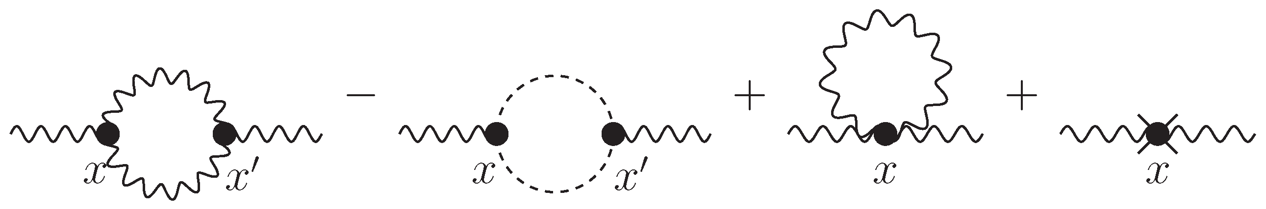
Although the nonlocal contributions obey the Ward identity away from coincidence, there is a local obstacle proportional to $ln\left(a\right){\delta }^4(x-x^{\prime })$. This obstacle might originate from anomalous contributions (68) to the first two diagrams of Figure 1. Such diagrams would contribute $ln\left(a\right){\delta }^4(x-x^{\prime })$ terms, which we would not be able to recognize from the unregulated, noncoincident result. It is also possible that we have missed some exotic, local contributions to the Feynman rules associated with the functional measure factor or time-ordering. More work is required to resolve this issue, and we believe a good venue for this study is the much simpler contribution to $-i\left[{}^{\mu \nu }{\Sigma }^{\rho \sigma }\right](x;x^{\prime })$ arising from a loop of massless, minimally coupled scalars [22]. Fortunately, the missing local terms do not make leading-order contributions to the gravitational potentials.

In Section 3, we applied our result to work out the gravitational response to a static point mass (70) at one loop. Because the graviton self-energy was computed in a fixed gauge, we had to solve the effective field equations using the same gauge fixing functional [3,4]. This resulted in there being four scalar potentials (71), instead of the usual two. Our final results for the leading late time forms of the four potentials were given in Equations (101)–(104). Of particular interest are the Newtonian potential and the gravitational slip:

$$\begin{array}{ccc}\hfill \mathrm{\Psi }& ⟶& \frac{GM}{ar}\left\{1+\frac{8G{H}^2}{\pi }\left[-{ln}^3\left(a\right)+3ln\left(a\right)ln\left(Hr\right)\right]+\dots \right\},\hfill \end{array}$$

(105)

$$\begin{array}{ccc}\hfill \mathrm{\Psi }-\mathrm{\Phi }& ⟶& \frac{GM}{ar}\left\{0+\frac{8G{H}^2}{\pi }\left[4{ln}^2\left(a\right)-3ln\left(Hr\right)\right]+\dots \right\}.\hfill \end{array}$$

(106)

It is interesting to compare the effect of graviton contributions to the Newtonian potential (105) with that from a loop of massless, minimally coupled scalars [23]:

$${\mathrm{\Psi }}_{MMCS}⟶\frac{GM}{ar}\left\{1-\frac{G{H}^2}{10\pi }\left[\frac{1}{3}ln\left(a\right)+3ln\left(aHr\right)\right]+\dots \right\}.$$

(107)

In both cases, the one-loop correction reduces the gravitational potential, but gravitons induce two additional factors of $ln\left(a\right)$. The same pattern is evident for the gravitational slip, which obtains two factors of $ln\left(a\right)$ from gravitons, but none at all from scalars [23]. Similarly, the one-loop correction to the graviton mode function is enhanced by ${ln}^2\left(a\right)$ [12], but is not affected at all by scalars [24]. We therefore conclude that loops of inflationary gravitons contribute more strongly than matter loops by two large logarithms. It is also noteworthy that graviton loop corrections to gravity are much stronger than graviton loop corrections to fermions [25,26,27], to electrodynamics [28,29,30,31,32], and to massless, minimally coupled scalars [33,34,35]. The key difference seems to be that graviton loop corrections to gravity can involve two graviton propagators, whereas graviton corrections to other fields involve only one.

The appearance of very large logarithms in graviton loop corrections implies the breakdown of perturbation at late times and large distances. It has been difficult to devise a resummation procedure because these logarithms derive from two sources: the “tail” part of the graviton propagator and logarithmic ultraviolet divergences of the form (49) [36]. This led to the speculation that resummation might be accomplished by combining a variant of Starobinsky’s stochastic formalism [37,38] with a variant of the renormalization group. This speculation was recently confirmed in the context of nonlinear sigma models on a nondynamical de Sitter background [39], which possess the same kinds of derivative interactions as quantum gravity and exhibit the same mixture of “tail” and ultraviolet logarithms. The technique has been applied to explain graviton loop corrections to the exchange potential of a massless, minimally coupled scalar [35], and strenuous efforts are underway to devise similar explanations for the collection of large graviton logarithms that have been patiently accumulated by direct computation over the course of two decades.

It is well known that classical modified gravity models also correct the force of gravity [40] and can induce nonzero gravitational slip [41,42]. One is therefore led to wonder if our results (105) and (106) could be reproduced by some local, metric-based model. The answer seems to be no because the only stable, local, invariant, and metric-based modification of gravity is $f\left(R\right)$ gravity [43]. However, the modified force induced by these models on the de Sitter background depends only on the combination $aHr$ [40] and cannot reproduce the distinct ${ln}^3\left(a\right)$ and $ln\left(a\right)ln\left(Hr\right)$ terms of our result (105). It should also be noted that neither the scalar nor the tensor amplitudes in these models experience secular growth after horizon crossing [44], unlike the ${ln}^2\left(a\right)$ dependence we found previously [12].

We close by commenting on the gauge issue. On a flat space background, the graviton self-energy is known to be highly gauge dependent [45]. Because the $H\to 0$ limit of our result agrees with the flat space limit, our de Sitter graviton self-energy must inherit this gauge dependence. The large logarithms we have found all derive from terms that carry factors of $H^2$, and their gauge dependence is not known, although indications from gravity plus electromagnetism suggest that there is some [32]. A procedure was developed for removing this gauge dependence [46], which has been successfully applied on a flat space background to graviton loop corrections to the massless, minimally coupled scalar [46] and to electromagnetism [47]. The massless, minimally coupled scalar exchange potential was identified as the simplest venue for generalizing this technique to the de Sitter background [35], and it is hoped that a result will be available later this year. Based on flat space background experience [46,47], we expect that the elimination of gauge dependence will not eliminate large graviton logarithms, but might change their numerical coefficients.

References

1. Starobinsky, A.A. Spectrum of relict gravitational radiation and the early state of the universe. JETP Lett. 1979, 30, 682–685. [Google Scholar]
2. Starobinsky, A.A. Cosmic Background Anisotropy Induced by Isotropic Flat-Spectrum Gravitational-Wave Perturbations. Sov. Astron. Lett. 1985, 11, 133. [Google Scholar]
3. Tsamis, N.C.; Woodard, R.P. The Structure of perturbative quantum gravity on a De Sitter background. Commun. Math. Phys. 1994, 162, 217–248. [Google Scholar] [CrossRef]
4. Woodard, R.P. de Sitter breaking in field theory. arXiv 2006, arXiv:gr-qc/0408002 [gr-qc]. [Google Scholar]
5. Iliopoulos, J.; Tomaras, T.N.; Tsamis, N.C.; Woodard, R.P. Perturbative quantum gravity and Newton’s law on a flat Robertson-Walker background. Nucl. Phys. B 1998, 534, 419–446, [arXiv:gr-qc/9801028 [gr-qc]]. [Google Scholar] [CrossRef] [Green Version]
6. Abramo, L.R.; Woodard, R.P. No one loop back reaction in chaotic inflation. Phys. Rev. D 2002, 65, 063515, [arXiv:astro-ph/0109272 [astro-ph]]. [Google Scholar] [CrossRef] [Green Version]
7. Tsamis, N.C.; Woodard, R.P. One loop graviton selfenergy in a locally de Sitter background. Phys. Rev. D 1996, 54, 2621–2639, [arXiv:hep-ph/9602317 [hep-ph]]. [Google Scholar] [CrossRef] [Green Version]
8. Tan, L.; Tsamis, N.C.; Woodard, R.P. Graviton self-energy from gravitons in cosmology. Class. Quant. Grav. 2021, 38, 145024, [arXiv:2103.08547 [gr-qc]]. [Google Scholar] [CrossRef]
9. Tsamis, N.C.; Woodard, R.P. The Quantum gravitational back reaction on inflation. Ann. Phys. 1997, 253, 1–54, [arXiv:hep-ph/9602316 [hep-ph]]. [Google Scholar] [CrossRef] [Green Version]
10. Onemli, V.K.; Woodard, R.P. Superacceleration from massless, minimally coupled phi**4. Class. Quant. Grav. 2002, 19, 4607, [arXiv:gr-qc/0204065 [gr-qc]]. [Google Scholar] [CrossRef] [Green Version]
11. Onemli, V.K.; Woodard, R.P. Quantum effects can render w < -1 on cosmological scales. Phys. Rev. D 2004, 70, 107301, [arXiv:gr-qc/0406098 [gr-qc]]. [Google Scholar] [CrossRef] [Green Version]
12. Tan, L.; Tsamis, N.C.; Woodard, R.P. How Inflationary Gravitons Affect Gravitational Radiation. Phil. Trans. R. Soc. 2021, 380, 0187, [arXiv:2107.13905 [gr-qc]]. [Google Scholar] [CrossRef]
13. Schwinger, J.S. Brownian motion of a quantum oscillator. J. Math. Phys. 1961, 2, 407–432. [Google Scholar] [CrossRef]
14. Mahanthappa, K.T. Multiple production of photons in quantum electrodynamics. Phys. Rev. 1962, 126, 329–340. [Google Scholar] [CrossRef]
15. Bakshi, P.M.; Mahanthappa, K.T. Expectation value formalism in quantum field theory. 1. J. Math. Phys. 1963, 4, 1–11. [Google Scholar] [CrossRef]
16. Bakshi, P.M.; Mahanthappa, K.T. Expectation value formalism in quantum field theory. 2. J. Math. Phys. 1963, 4, 12–16. [Google Scholar] [CrossRef]
17. Keldysh, L.V. Diagram technique for nonequilibrium processes. Zh. Eksp. Teor. Fiz. 1964, 47, 1515–1527. [Google Scholar]
18. Chou, K.C.; Su, Z.B.; Hao, B.L.; Yu, L. Equilibrium and Nonequilibrium Formalisms Made Unified. Phys. Rep. 1985, 118, 1–131. [Google Scholar] [CrossRef]
19. Jordan, R.D. Effective Field Equations for Expectation Values. Phys. Rev. D 1986, 33, 444–454. [Google Scholar] [CrossRef]
20. Calzetta, E.; Hu, B.L. Closed Time Path Functional Formalism in Curved Space-Time: Application to Cosmological Back Reaction Problems. Phys. Rev. D 1987, 35, 495. [Google Scholar] [CrossRef]
21. Ford, L.H.; Woodard, R.P. Stress tensor correlators in the Schwinger–Keldysh formalism. Class. Quant. Grav. 2005, 22, 1637–1647, [arXiv:gr-qc/0411003 [gr-qc]]. [Google Scholar] [CrossRef] [Green Version]
22. Park, S.; Woodard, R.P. Scalar Contribution to the Graviton Self-Energy during Inflation. Phys. Rev. D 2011, 83, 084049, [arXiv:1101.5804 [gr-qc]]. [Google Scholar] [CrossRef] [Green Version]
23. Park, S.; Prokopec, T.; Woodard, R.P. Quantum Scalar Corrections to the Gravitational Potentials on de Sitter Background. J. High Energy Phys. 2016, 1, 074, [arXiv:1510.03352 [gr-qc]]. [Google Scholar] [CrossRef] [Green Version]
24. Park, S.; Woodard, R.P. Inflationary Scalars Don’t Affect Gravitons at One Loop. Phys. Rev. D 2011, 84, 124058, [arXiv:1109.4187 [gr-qc]]. [Google Scholar] [CrossRef] [Green Version]
25. Miao, S.P.; Woodard, R.P. The Fermion self-energy during inflation. Class. Quant. Grav. 2006, 23, 1721–1762, [arXiv:gr-qc/0511140 [gr-qc]]. [Google Scholar] [CrossRef]
26. Miao, S.P.; Woodard, R.P. Gravitons Enhance Fermions during Inflation. Phys. Rev. D 2006, 74, 024021, [arXiv:gr-qc/0603135 [gr-qc]]. [Google Scholar] [CrossRef] [Green Version]
27. Miao, S.P. Quantum Gravitational Effects on Massive Fermions during Inflation I. Phys. Rev. D 2012, 86, 104051, [arXiv:1207.5241 [gr-qc]]. [Google Scholar] [CrossRef] [Green Version]
28. Leonard, K.E.; Woodard, R.P. Graviton Corrections to Vacuum Polarization during Inflation. Class. Quant. Grav. 2014, 31, 015010, [arXiv:1304.7265 [gr-qc]]. [Google Scholar] [CrossRef] [Green Version]
29. Glavan, D.; Miao, S.P.; Prokopec, T.; Woodard, R.P. Electrodynamic Effects of Inflationary Gravitons. Class. Quant. Grav. 2014, 31, 175002, [arXiv:1308.3453 [gr-qc]]. [Google Scholar] [CrossRef] [Green Version]
30. Wang, C.L.; Woodard, R.P. Excitation of Photons by Inflationary Gravitons. Phys. Rev. D 2015, 91, 124054, [arXiv:1408.1448 [gr-qc]]. [Google Scholar] [CrossRef] [Green Version]
31. Glavan, D.; Miao, S.P.; Prokopec, T.; Woodard, R.P. Graviton Loop Corrections to Vacuum Polarization in de Sitter in a General Covariant Gauge. Class. Quant. Grav. 2015, 32, 195014, [arXiv:1504.00894 [gr-qc]]. [Google Scholar] [CrossRef] [Green Version]
32. Glavan, D.; Miao, S.P.; Prokopec, T.; Woodard, R.P. One loop graviton corrections to dynamical photons in de Sitter. Class. Quant. Grav. 2017, 34, 085002, [arXiv:1609.00386 [gr-qc]]. [Google Scholar] [CrossRef] [Green Version]
33. Kahya, E.O.; Woodard, R.P. Quantum Gravity Corrections to the One Loop Scalar Self-Mass during Inflation. Phys. Rev. D 2007, 76, 124005, [arXiv:0709.0536 [gr-qc]]. [Google Scholar] [CrossRef] [Green Version]
34. Kahya, E.O.; Woodard, R.P. Scalar field equations from quantum gravity during inflation. Phys. Rev. D 2008, 77, 084012, [arXiv:0710.5282 [gr-qc]]. [Google Scholar] [CrossRef] [Green Version]
35. Glavan, D.; Miao, S.P.; Prokopec, T.; Woodard, R.P. Large logarithms from quantum gravitational corrections to a massless, minimally coupled scalar on de Sitter. J. High Energy Phys. 2022, 3, 088, [arXiv:2112.00959 [gr-qc]]. [Google Scholar] [CrossRef]
36. Miao, S.P.; Prokopec, T.; Woodard, R.P. Scalar enhancement of the photon electric field by the tail of the graviton propagator. Phys. Rev. D 2018, 98, 025022, [arXiv:1806.00742 [gr-qc]]. [Google Scholar] [CrossRef] [Green Version]
37. Starobinsky, A.A. Stochastic de sitter (inflationary) stage in the early universe. Lect. Notes Phys. 1986, 246, 107–126. [Google Scholar] [CrossRef]
38. Starobinsky, A.A.; Yokoyama, J. Equilibrium state of a selfinteracting scalar field in the De Sitter background. Phys. Rev. D 1994, 50, 6357–6368, [arXiv:astro-ph/9407016 [astro-ph]]. [Google Scholar] [CrossRef] [Green Version]
39. Miao, S.P.; Tsamis, N.C.; Woodard, R.P. Summing inflationary logarithms in nonlinear sigma models. J. High Energy Phys. 2022, 3, 069, [arXiv:2110.08715 [gr-qc]]. [Google Scholar] [CrossRef]
40. Soussa, M.E.; Woodard, R.P. The force of gravity from a Lagrangian containing inverse powers of the ricci scalar. Gen. Rel. Grav. 2004, 36, 855–862, [arXiv:astro-ph/0308114 [astro-ph]]. [Google Scholar] [CrossRef] [Green Version]
41. Nojiri, S.; Odintsov, S.D. Unified cosmic history in modified gravity: From F(R) theory to Lorentz non-invariant models. Phys. Rep. 2011, 505, 59–144, [arXiv:1011.0544 [gr-qc]]. [Google Scholar] [CrossRef] [Green Version]
42. Capozziello, S.; Laurentis, M.D. Extended Theories of Gravity. Phys. Rep. 2011, 509, 167–321, [arXiv:1108.6266 [gr-qc]]. [Google Scholar] [CrossRef] [Green Version]
43. Woodard, R.P. Avoiding dark energy with 1/r modifications of gravity. Lect. Notes Phys. 2007, 720, 403–433, [arXiv:astro-ph/0601672 [astro-ph]]. [Google Scholar] [CrossRef] [Green Version]
44. Brooker, D.J.; Odintsov, S.D.; Woodard, R.P. Precision predictions for the primordial power spectra from f(R) models of inflation. Nucl. Phys. B 2016, 911, 318–337, [arXiv:1606.05879 [gr-qc]]. [Google Scholar] [CrossRef] [Green Version]
45. Capper, D.M. On quantum corrections to the graviton propagator. Nuovo Cim. A 1975, 25, 29. [Google Scholar] [CrossRef]
46. Miao, S.P.; Prokopec, T.; Woodard, R.P. Deducing Cosmological Observables from the S-matrix. Phys. Rev. D 2017, 96, 104029, [arXiv:1708.06239 [gr-qc]]. [Google Scholar] [CrossRef] [Green Version]
47. Katuwal, S.; Woodard, R.P. Gauge independent quantum gravitational corrections to Maxwell’s equation. J. High Energy Phys. 2020, 21, 029, [arXiv:2107.13341 [gr-qc]]. [Google Scholar] [CrossRef]
Figure 1. Diagrams contributing to the one-loop graviton self-energy, shown in the same order, left to right, as the four contributions to (15). Graviton lines are wavy and ghost lines are dashed.
Universe 08 00376 g001