1. Introduction
Supernovae are produced by stars that end their late evolution in a catastrophic explosive process. The work [
1] introduces the name supernova (SN) and defines the difference between SNe and novae in terms of their estimated explosive powers. The luminosity of a SN at its maximum, which lasts for several days, is comparable to the total luminosity of its host galaxy. There are two general types of a SN, classified according to the presence of hydrogen absorption lines in the observed spectrum. Absorption lines are present in the spectra of Type II SNe and absent in the spectra of Type I SNe. In addition, Type II SNe normally contain compact remnants. Type I SN is associated with thermonuclear explosions in a binary system, while Type II is the result of the core collapse of massive stars with mass ≳10
.
In this article, I discuss Type II SNe. The thermonuclear burning in the center of massive stars gives us an iron core with a mass
–
and with a radius ∼
cm [
2]. At such densities, mainly degenerate relativistic electron gas provides pressure, preventing the gravitational collapse of the iron core. The relativistic adiabatic index
is the boundary of stability region against the collapse. The iron core collapses due to the neutrinos loosening. The energy is carried away by neutrinos. The total energy carried by neutrinos can be estimated as a gravitational energy of the forming neutron star with a mass
and a radius
∼10 km, i.e., neutrinos carry out
∼
erg over a few seconds. The neutrino energy is ∼100 MeV per nucleon, while thermonuclear energy can provide at least one order less (8 MeV per nucleon). Due to the different timescales of core collapse and light curves from SNe, it is possible divide the problem of the collapse from the simulation of light curves. The simulation of light curves proves a small part of energy of neutrinos absorbed by the matter of the collapsing core envelope ∼
erg, less than 1% of full energy [
3].
The work [
4] was the first to investigate the spherically symmetric problem of the core collapse calculations. Authors overestimated the transparency of matter for the neutrino and obtained the necessary energy deposition for SNe explosion due to a large average energy of the emitted neutrino. The mathematical model of neutrino heat conductivity suitable for calculations with available computing power was formulated in [
5,
6]. The model introduces a neutrinosphere, opaque and transparent regions for neutrinos. The model demonstrates the disadvantage of the spherically symmetric problem for explanation of SNe explosion. Moreover, the 1D model gives low average energies of emitted neutrinos ∼5 MeV in comparison with more complicated spherically symmetric models taking into account kinetic Bolzmann equations for neutrino transport [
7,
8,
9,
10,
11].
The reason for the uncertainty in the construction of a model for the explosion of SNe [
3,
12,
13] is the difficulties of a mathematical problem. One needs to take into account hydrodynamics for the matter and kinetic Boltzmann neutrino transport with different time scales and different space scales. Matter density changes from the densities of white drafts with degenerate relativistic electrons to the degenerate nuclear densities of forming neutron stars that are nontransparent for neutrinos. In addition, multidimensionality and instabilities during collapse play an important role. Regions of convective instabilities with the entropy gradient collinear with gravitational acceleration are forming during the collapse, grads
. Because the center contains high-energy neutrinos, convection in multidimensional simulations gives us a higher neutrino energy flux in comparison with 1D [
14,
15]. As a results, some 2D [
16,
17] and 3D [
18,
19] models provide the SN explosion, while other models [
20,
21,
22] cannot demonstrate the necessary energy deposition ∼10
erg. Because the cited works do not include the neutrino spectrum, it would be useful to indicate only the correlation between large scale convection and obtained explosion.
Large scale convection at the center of a star was first investigated in 3D hydrodynamic calculations in [
23] for a stationary initial state with an arbitrary uniform entropy in the center and an ideal gas low equation of state. In 3D hydrodynamic calculations without neutrino transport [
24,
25] we considered the convection for a more realistic entropy distribution in the initial state corresponding to 1D calculations for a full input physics. Used ideal gas equation of state is appropriate for Fermi–Dirac statistic of relativistic electrons for any degree of degeneracy, in case we are using only the relation between pressure and internal specific energy without temperature. We also included neutrino transport, simplified reactions of weak interactions, and realistic equation of state for the matter at high energy density in [
26]. We proved the assumption about the applicability of Schwarzschild’s convective instability criterion for gas dynamics,
, near the neutrinosphere of the forming proto-neutron star due to nonequilibrium nonreversible neutronization, i.e., the loss of neutrinos.
The main expected effects from large-scale convection are not only the increasing of the neutrino energy flux, but also the increasing of the average energy for outgoing neutrinos, because large-scale convection facilitates the neutrino transport from a “hot” central region. The average neutrino energy 30 MeV, even with the same neutrino luminosity such as a 1D model of collapse, provides the kinetic energy of the envelope ∼
erg [
24], because the cross section of neutrino scattering on electron with the small Fermi energy is proportional to the average neutrino energy [
27,
28,
29]. To understand the possibility of such important effect due to convection, we calculated 2D collapse with neutrino spectrum [
30,
31]. We obtained the energy of outgoing neutrinos ∼15 MeV due to convection in compare with ∼10 MeV in 1D calculations without convection [
27]. Moreover, we proved by means of 3D calculations with neutrino energy transport and without neutrino spectrum [
32] that slow differential rotation make 3D calculations close to 2D as predicted author [
33].
In this work I discuss the original mathematical model of the multidimensional multitemperature gas dynamic with neutrino transfer. I analyze nonequlibrium neutranization in gravitational collapse in the more accurate computational grid in comparison with [
31]. I focus on the neutrino spectrum only, excluding the interaction of the outgoing neutrinos with the shell. This limitation considerably simplifies the model of the interaction of neutrinos with matter and the grid size of the computational region.
The emitted neutrinos spectrum prediction is the most important theoretical result for the future registration of neutrinos. In my opinion, the registration of SN neutrino spectrum is very important for confirmation of the model of collapse and SN. Unfortunately, only few neutrino events were detected from a close SN, 1987A, in a neighboring galaxy. Another feature of SN1987A is the orientation toward the southern hemisphere of the Earth, because the registered outgoing particles of weak interaction matter with the SN neutrino can be observed by the neutrino observatories located the in the northern hemisphere of the Earth. The first publications indicate high neutrino energies: 20–40 MeV IMB [
34], 9–35 MeV Kamiokande-II [
35], and 20 MeV Baksan-LSD [
36,
37], which is closer to the large scale convection model than to the spherically symmetric collapse. Admittedly, the registered neutrino events from SN1987A led to a significant increasing of the observed background level correlated with the SN light observed from the southern hemisphere of the Earth. The registration of neutrino events also utilized mathematical models of core collapse [
38], sometimes 1D core collapse with average neutrino energy 5 MeV from the neutrinosphere. The interpretation of registered events is sensitive for the neutrino spectrum.
Modern neutrino observatories promise thousands of times more neutrino events from a close SN [
39]. New observatories operate with a large amount of working substance, but the number of events is very sensitive for the expected energy of incoming low-energy neutrinos for core collapse in comparison with high-energy neutrinos. For this reason, the simulations of core collapse are focused on prediction of the neutrino spectrum. In addition to that, the neutrino spectrum is important from the perspective of the large-scale convection and the mechanism of SNe explosion. Most modern core collapse simulations are focusing on multidimensional models with instabilities in 2D [
40] and 3D [
41] simulations. Such models give us average neutrino energy 15–20 MeV closer to our results with large-scale convection [
31]. Some of the modern simulations examine the impact of the nuclear equation of state on core collapse and the neutrino spectrum [
42].
2. Mathematical Model of Core Collapse with the Neutrino Transport
The physical problem of gravitational collapse includes the hydrodynamic equations for the matter with a self gravity and kinetic Boltzmann equations for distribution functions of different kinds of neutrinos. Matter includes electrons, positrons, free nucleons, nuclei, and photons. Matter can be described by hydrodynamics due to its small thermalization time. Neutrinos take part in weak interactions with matter, and may not be in thermal equilibrium; only at the forming of a proto-neutron star in the part of the computational region may a neutrino achieve equilibrium with matter.Weak interactions have interesting features of conservation of lepton number (difference between the number of leptons and the number of antileptons). For this reason, in hydrodynamic equations one has the additional value difference between an electron and a positron per nucleon, , below the named number of electrons. Weak interactions and neutrino transport changes the number of electrons in a moving fluid of matter.
For the multidimensional case, there is useful a model of flux-limited diffusion proposed for a spherically symmetric collapse in [
43]. The model does not include the dependence of distribution functions of the neutrino from various angles. In the opaque case, the neutrino spectral fluxes are defined by the gradients of the spectral energy densities. In the transparent region, the neutrino flux is proportional to the energy density. In a flux-limited diffusion model the fluxes are proportional to the gradients of the energy density, while the semi-transparent region contains an arbitrary interpolation of fluxes in transparent and opaque areas. The flux-limited diffusion is easily generalized for the multidimensional case. It also solves the problem of small timescales for reaction rates in opaque regions.
Multicomponent hydrodynamic code [
44,
45,
46] operates with independent variables: concentration densities
, internal energies
of components
i, momentum density
(the velocities of all components of matter are assumed to be the same). One has a system of Euler equations on a fixed coordinate system. Taking into account discontinuities, one should use conservative differential equations. The low conservation of the number of baryons is
the equation for the difference between the electrons and positron concentrations while taking into account reactions is
the equation for momentum of matter
with momentum flux density tensor in orthogonal coordinates
, the equation for the energy density of matter is
is the sum of specific internal and kinetic energies, and
is the heating of matter by neutrino. The acceleration of gravity is the potential gradient
, obtained from the numerical solution of the Poisson equation [
47]
The transport of neutrinos of type
is described by the kinetic Boltzmann equation
with emission and absorption coefficients
,
, in reaction
q.
It is necessary to introduce a grid for neutrino energies and use the spectral energy densities of neutrinos and antineutrinos disregarding the angular dependence of the distribution function,
in each interval of the grid for neutrino energy
. I do not consider antineutrinos separately from neutrinos. I will adopt the same distribution functions in the laboratory and matter-accompanying reference frames (for nonrelativistic velocities
). The equilibrium neutrino spectrum is
The transport equation for the spectral energy density is
where
, the spectral flux is determined by the gradient of spectral energy density. In the opaque case, one has the diffusion approximation
; in the transparent case, the flux is limited only the speed of light for neutrinos
. In an arbitrary case, some arbitrary interpolations of fluxes is used (so-called flux-limiting)
A nonlinear diffusion coefficient transforms the diffusion (parabolic) equation in the opaque region to the transport (hyperbolic) in the transparent region.
The energy exchange between neutrinos and matter provide relaxation to equilibrium
where the equilibrium neutrino energy is defined by the energy conservation
The relaxation rate was chosen proportional to the concentration of free nucleons (
) with constant cross section
. This model gives us the spectrum of outgoing neutrinos, but a constant cross section is not sufficient to describe their absorption in the envelope. The cross section for scattering with electrons of the envelope for energies of outgoing neutrinos of 10 MeV (much higher than the Fermi energy electrons) is proportional to the neutrino energy [
27].
3. The Equation of State and an Initial Model
The equation of state (EOS) of matter represents coupled equations for pressure (
) and internal energy (
) as functions of density, temperature and in our case of a week interaction also number of electrons (
)
Matter includes nuclei with free nucleons in statistical equilibrium, pairs and equilibrium radiation. The statistical equilibrium nuclei (mass numbers
, charges
) with free nucleons:
gives the relation of chemical potentials
where the chemical potential
i-nuclei can be defined in non-relativistic case (with taking into account degeneracy of Fermi particles) from relation
with number densities of nuclei
, Fermi-Dirac function
of order
and statical weight
. The sum of number densities equals to one
while the electroneutrality gives the relation
Pressure and specific internal energy of nucleons are described by equations
For nuclei, it is not necessary to take into account degeneracy, as it can be described by ideal gas low EOS. Radiation is the black body.
For electrons, one can use EOS of ultra-relativistic pairs (
):
In is interesting to note that an ideal gas relation between pressure and internal energy for ultra-relativistic Fermi particles is true for any degree of degeneracy
with adiabatic index
. In the case of non relativistic case at any degree of degeneracy adiabatic index is
. Without reactions and neutrino transport the ideal conservative hydrodynamic is a suitable approach [
25].
In the conservative scheme, the independent variables are
, so one needs to resolve matter temperature,
T, from a nonlinear EOS (
13) by a Newton iterations with taking into account electro neutrality condition (
19).
The number of electrons
is determined from the kinetics of neutronization
Strictly speaking, in EOS only pair plasma is ultra relativistic. Nucleons are not relativistic, but become degenerate at high densities. Nuclei are not relativistic and they are not degenerate.
In a simplified description of kinetics I take into account the relaxation of number of electrons,
, to
-equilibrium
from [
48]
with two reactions being considered,
in the assumption of a free escape of neutrinos. Such a model is quantitatively exact only in the transparent region near the neutrinosphere. In an opaque region, a simple model of equilibrium is only qualitatively true, but the neutrino energy fluxes in the opaque region are also negligibly small. Quantitatively, such a simplified model of neutronization in an opaque region has no effect on outgoing neutrino spectrum [
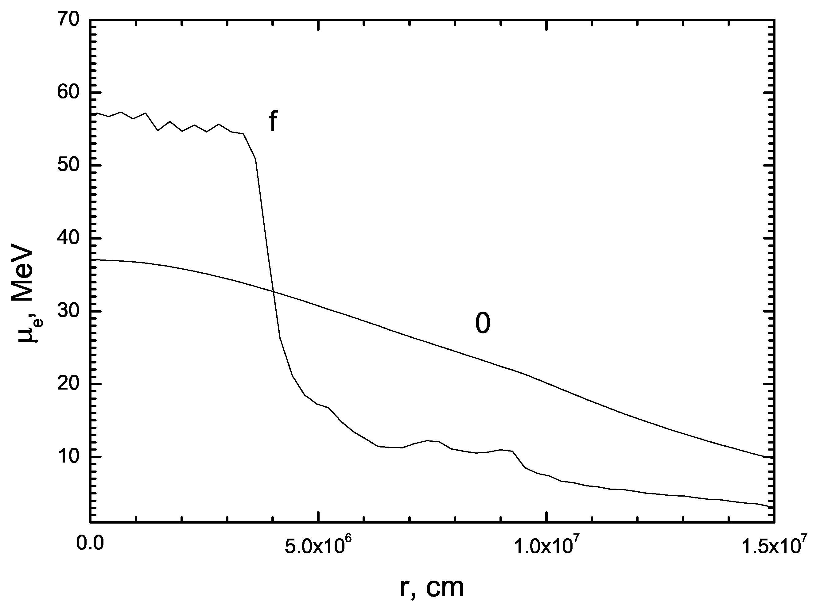
31]. It is possible to make the simple neutronization model true by means of correction the lower boundary limit for an equilibrium electron number
. This correction provides a realistic electron chemical potential at the collapse at high density in
Figure 1 as in the spherically symmetric calculation of the collapse with full input physics [
27].
Because degenerate relativistic electrons a play main role in EOS in the initial state of collapse, the relationship between pressure and density as in the polytrope
with index
may be taken as the initial data. Moreover, including slow initial rotation provides us 2D axial symmetry even in 3D consideration [
32]. I consider it in initial model already on the stage of collapse, and rotation is differential. The low rotation is a constant ratio of centrifugal force to gravity (called
-constant rotation low in [
49]). In the selected differential rotation, rotation effects affect the central region where convection is of interest, but the measure of rotation, the rotation energy, is small,
(the ratio of the polar radius to the equatorial radius is 0.9). The angular velocity in the forming neutron star reaches
at the end of calculations 12 ms, the center part makes less than one revolution during this time.
The polytropic initial model contains three independent physical parameters, for example, the gravitational constant
G, central density
, and equatorial radius
. I chose center density
in the initial model, large enough for neutronization. For fixed mass
, the polytrope initial model gives the equatorial radius
cm, gravitational energy
erg, rotational energy
. The chosen central density in the initial equilibrium corresponds to the ongoing collapse of the real core of a star. The small initial radius of already ongoing collapse of the real core makes it possible to use a smaller fixed Euler computational grid. It is possible to resolve a neutron star formation on a fixed computational grid. In reality, the collapse begins at the radius of the star ∼
cm; and the initial stage of neutrino energy losses over a long period of a few seconds significantly exceeds the gas dynamic time
for real low initial central density ∼
[
27].
For the dimensional values of density and pressure in the initial model, it is necessary to recalculate
and temperature
. Such an initial model provides the exact mathematical equilibrium without the neutrino transfer. In the initial state, I obtain the same entropy profile decreasing at the center
(see
Figure 2), as in the spherically symmetric collapse calculation with a full input physics during ∼10 ms [
27].
The decreasing entropy profile is a result of neutronization. Weak interactions reduce the number of electrons , and the specific energy is transferred from the electronic component to the nucleons. This probably convective instability region () is interesting to study in a scale of convection. Large-scale convection can produce outgoing neutrinos with high energies.
For calculating the 2D problem in spherical coordinates
, a
grid was used for a part of the polytrope (the computational domain is limited to
) under the assumption of axial symmetry
and the plane of symmetry
. The angular variable contains more intervals in compare with our recent calculations [
31] to resolve possible low-scale instabilities. The grid of 15 intervals from 0 up to 40 MeV is used to carry spectral neutrino energy density. At the outer boundary, there is a non-flow smooth wall for matter. Neutrinos freely leave the computational region. Numerical nonconservation of the component of the angular momentum
of matter is associated with approximation errors of the scheme, nonconservation is small enouugh [
25].
To prevent small time steps of an explicit hydrodynamic scheme due to Courant condition of the stability I split the time steps for numerical integrations along the angular for a small radius.
The computational method uses splitting with respect to the physical processes. The hydrodynamic transport is based on an explicit conservative scheme and an original Riemann problem solver for a multicomponent gas mixture with a tabular EOS [
44,
45] (see also
Appendix A). The processes of energy exchange between the components (matter and neutrinos) are considered at a separate time step using the implicit Gear’s method [
50]. Moreover, the neutrino diffusion term is considered by lines method [
45] and in implicit Gear’s method. Key point of the method is joint consideration of matter and neutrinos in conservative hydrodynamic equations. In the opaque region hydrodynamics weakly affect the equilibrium, and the reactions of weak interaction, calculated by an implicit method at a separate step. Small timescales of reactions do not affect the number of time steps of gas-dynamic transport. In the case of opaque neutrino hydrodynamic time steps, they are determined by hydrodynamic Courant conditions of numerical stability,
, with the speed of sound and velocity of matter. The only significant limitation on the time step,
, in comparison with gas dynamics arises in the transparent region, where the neutrino transport speed (speed of light
c) is at least an order of magnitude greater than the speed of sound and the gas dynamic speed of matter because of accuracy requirements, not numerical stability.
There is only one alternative in the literature: the Castro code [
17], which differs by an approximate Riemann problem solver. Other gas dynamic models for calculating collapse use a separate description of gas dynamics for matter and neutrino transport, for example, the Fornax code [
51]. From the point of view of mathematics, the difference from the joint description of neutrinos and matter in gas dynamics is not fundamental. However, in calculations of a real problem in the optically dense region, the number of time steps for calculating the energy exchange between neutrinos of different energies will depend on the timescale of the fastest reaction.
I would like to make remark about the controversial properties of the calculations for degenerate matter. A conservative scheme solves the problem of time steps for the opaque region, in which the time steps are determined only by the gas dynamic transport and the speed of sound. For a small numerical errors of determining the specific energy of matter, the resulting temperature errors are large because of degeneracy pairs. For the used computational grid, it is possible to calculate the development of instability for strong degeneracy
∼60 MeV at temperature
MeV.
Figure 1 demonstrates some artifact numerical oscillations of the chemical potential of electrons
MeV in the center at final time because of the loss of the accuracy of temperature. Strictly speaking, the forming at the collapse the proto-neutron core always is degenerate (due to degenerate both pairs and neutrons), but the proto-neutron star is not hot.
4. Results of Calculations
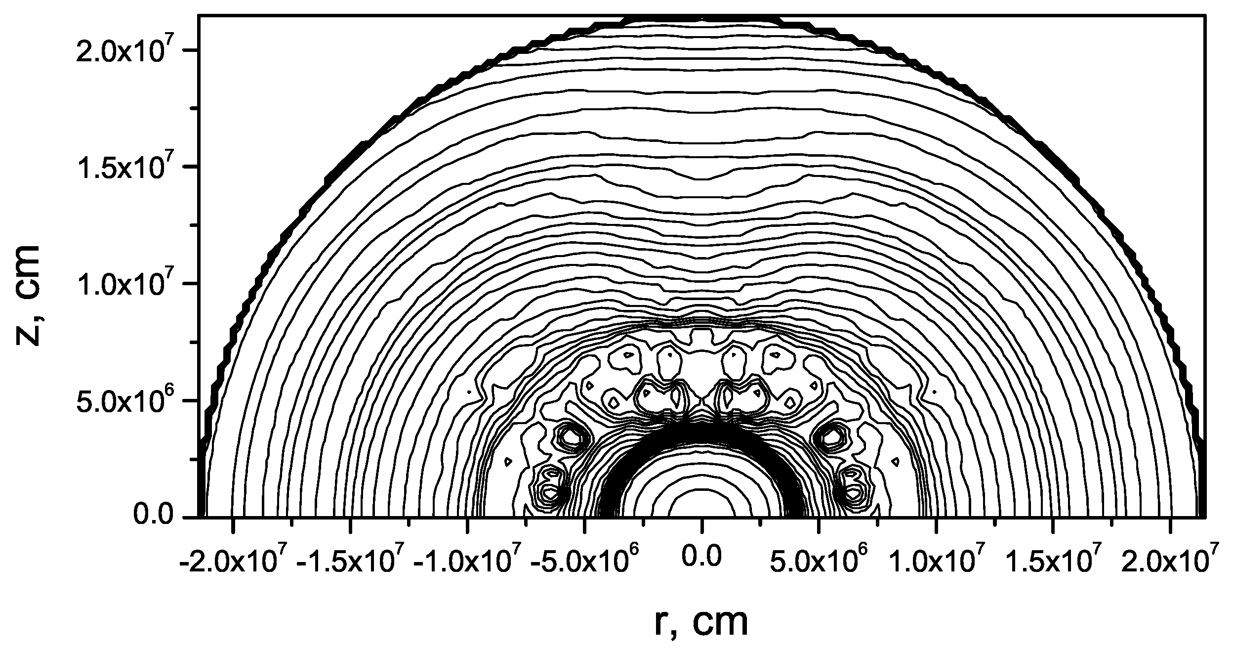
Due to neutrino losses, the pressure gradient can not keep a balance with gravity force, and matter collapses to the center. At collapse density increases, and neutrinos become trapped in the central region under the neutrinosphere. Contours of constant density in the equatorial plane in
Figure 3 at time
ms show the development of large scale convection in accordance with the gas dynamic time is
ms for average density
near the neutrinosphere.
The initial state contains unstable entropy profile
(
Figure 2). A rearrangement of decreasing entropy profile near the photosphere indicates the convection in this region in accordance with the Schwarzschild instability condition [
52]. The semitransparent region of nonequilibrium irreversible neutronization near the neutrinosphere specifies the scale of the convection without the dependence of grid size. Different computational grids
(present calculations) and
in [
31,
32]) provide approximately the same four “hot” bubbles above neutrinosphere in the angle interval
in
Figure 3. Thickness of the semitransparent region and slow differential rotation (see also 3D calculations in [
25,
32]) form long-wavelength perturbations.
In the central part under the neutrinosphere, neutrinos are captured by matter, neutronization is in equilibrium and reversible, and convection develops worse as in the Ledoux stability criterion [
53]. The Ledoux stability criterion takes into account the chemistry of the matter. With trapped neutrinos, the problem about stability becomes a strict stability problem. The artificial shutdown of the neutrino transport demonstrates a long time for development of the convection (∼100 ms). If one recalculates specific entropy removing the number of electrons
from the problem in the assumption of fast relaxation of
to the equilibrium value
, the unstable entropy profile will disappear.
Figure 4 shows the spectral neutrino flux
near the neutrinosphere
cm above the neutrinosphere at time 12 ms. The maximum spectral luminosity is reached at 18 MeV, while an average neutrino energy (the ratio of the energy flux to the particle flux) is 15 MeV. The spectrum of outgoing neutrinos becomes harder in comparison with the spherically symmetric calculation due to convection in the central region with high-energy neutrinos trapped in optically dense matter in 1D [
27] by a factor of
. The energy 18 MeV of outgoing neutrinos corresponds to the chemical potential of electrons at time 12 ms in
Figure 1 in the convective region near the neutrinosphere. The convection does not affect the center with a high chemical potential.
The axially symmetric calculations of the authors in [
17,
54] gives a similar result in terms of the average neutrino energies as the result presented here 12–20. Moreover, calculations by [
17,
54] give a higher neutrino luminosity in comparison with the spherically symmetric model.
Recent investigations are focusing on the possibility of detecting neutrinos from collapsing supernovae from a new neutrino observatory [
39]. The calculation of the neutrino spectrum becomes no less important than the SN mechanism. The average neutrino energies at the level of 5–10 MeV give a significantly lower rate of detected events and will to be distinguishable from 15 MeV neutrinos. However, the energies of 30 MeV neutrinos (interesting from a viewpoint of the large-scale convection mechanism of the SN) may be indistinguishable from 15 MeV neutrinos at a registration [
39] because of possible neutrino oscillations. Then, if neutrino oscillations are allowable, the time-integrated neutrino spectrum can be reproduced by detecting neutrinos with several types of detectors [
54].


