A Three-Order, Divergence-Free Scheme for the Simulation of Solar Wind

Abstract

In this paper, we present a three-order, divergence-free finite volume scheme to simulate the steady state solar wind ambient. The divergence-free condition of the magnetic field is preserved by the constrained transport (CT) method. The CT method can keep the magnetic fields divergence free if the magnetic fields is divergence free initially. Thus, a least-squares reconstruction of magnetic field with the divergence free constraints is used to make the magnetic fields global solenoidality initially. High order spatial accuracy is obtained through a non-oscillatory hierarchical reconstruction, while a high order time discretization is achieved using a three-order Runge–Kutta scheme. This new model of three order in space and time is validated by numerical results for Carrington rotation 2207. The numerical results show its capability for producing stable reliable results for structured solar wind. The high-order, divergence-free properties of this method make it an ideal tool for the simulations of coronal mass ejection in future.

1. Introduction

The modelling of astrophysical phenomena including jets, accretion disks, winds, solar flares, and magnetospheres has prompted the search for efficient and accurate numerical formulations for solving the magnetohydrodynamics (MHD) equations. The current status of MHD simulations for space weather is reviewed in the recent book of Feng [1]. Numerical computations based on finite volume (FV) discretization are powerful numerical methods for solving the MHD equations. It evolves only cell averages of a solution over time and can preserve the conservation of relevant physical quantities such as mass, momentum and energy.

High-order numerical methods have gained popularity in the last years because they are more efficient at capturing the rich structure in space weather phenomena than the low-order method [2,3,4,5,6,7,8,9]. To achieve high order accuracy, the high order reconstructions such as the k-exact reconstruction, the Essentially Non-Oscillatory (ENO) [10], Weighted Essentially Non-Oscillatory (WENO) [11,12], Total Variation Diminishing (TVD) [13] and Piecewise Parabolic Method (PPM) [13,14] reconstructions have been developed. In a series of works, discontinuous Galerkin (DG) methods have been developed for nonlinear conservation laws and related equations [15,16,17,18]. Compared to FV schemes, DG stores and evolves every polynomial coefficient in a cell over time. When the reconstruction order becomes higher, to remove spurious oscillations and maintain the high resolution near discontinuities, a nonlinear limiting procedure or characteristic decomposition is usually necessary.

Recently, ref. [19] proposed a new FV approach by using the hierarchical non-oscillatory reconstruction to remove the spurious oscillations while maintaining the high resolution without characteristic decomposition. First, a high degree polynomial in each cell is reconstructed. These polynomials are not necessarily non-oscillatory. Then, the hierarchical reconstruction is applied to the piece-wise polynomial solution. Ref. [19] also demonstrated that this new FV scheme does not have significant spurious oscillations even for a formal order of accuracy as high as 5th order. Later, refs. [20,21] extends this central hierarchical non-oscillatory reconstruction to the MHD equations. Since the FV approach proposed by [19,20,21] has advantages over traditional high order numerical methods, such as its easy operation without characteristic decomposition, it simplifies the numerical calculations. Additionally, it has never been used to model the solar wind. Thus, we adapt the three order FV approach combined with the hierarchical non-oscillatory reconstruction to simulate the large-scale structure of solar wind. To maintain the positivity of density and pressure in the reconstruction process, a self-adjusting strategy proposed by [22] is also used in the reconstruction process.

The divergence free constraint on the magnetic field is another numerical challenge in the simulation of MHD. In the past decades, various methods have been developed to satisfy the $\nabla ·\mathbf{B}=0$ constraint in MHD calculations [23,24,25,26,27,28]. Using stagger mashes to control $\nabla ·\mathbf{B}$, the constrained transport (CT) method can maintain the magnetic field divergence around the machine round off error as long as the initial conditions are compatible with the constraints. Thus, we use the CT method to preserve the divergence-free condition of the magnetic field in this paper. As in [29,30], a least-squares reconstruction with the divergence free constraints is used to get the face average magnetic fields initially. The magnetic fields divergence error is around ${10}^{-12}$.

This paper is organized as follows. In Section 2, MHD equations for solar wind plasma in spherical coordinates are described. Section 3 is devoted to a grid system and the numerical scheme formulation. Section 4 presents the numerical results for steady-state solar wind structure. Finally, some conclusions are presented in Section 5.

2. Governing Equations

The magnetic field $\mathbf{B}$ is split as a sum of a time-independent potential magnetic field ${\mathbf{B}}_0$ and a time-dependent deviation ${\mathbf{B}}_1$ [27,31]. In the present paper, this physical splitting of the MHD equations into the fluid part and the magnetic part are considered in order to design efficient FV schemes with spatial discretization for the fluid equations and the magnetic induction equation adopted from [27]. The fluid part with the magnetic field becomes a source term in an extended Euler system reading as follows:

$$\frac{\partial \mathbf{U}}{\partial t}+\frac{1}{r^2}\frac{\partial }{\partial r}{r}^2\mathbf{F}+\frac{1}{rsin\theta }\frac{\partial }{\partial \theta }sin\theta \mathbf{G}+\frac{1}{rsin\theta }\frac{\partial }{\partial \varphi }\mathbf{H}=\mathbf{S}$$

(1)

$$\mathbf{F}=\left(\begin{array}{c}\rho v_r\\ \rho v_r^2+p+\frac{-B_{1r}^2+B_{1\theta }^2+B_{1\varphi }^2}{2\mu }+\frac{-B_{1r}{B}_{0r}+B_{1\theta }{B}_{0\theta }+B_{1\varphi }{B}_{0\varphi }}{\mu }\\ \rho v_r{v}_{\theta }-\frac{B_{1r}{B}_{1\theta }+B_{1r}{B}_{0\theta }+B_{0r}{B}_{1\theta }}{\mu }\\ \left(\rho v_r{v}_{\varphi }-\frac{B_{1r}{B}_{1\varphi }+B_{1r}{B}_{0\varphi }+B_{0r}{B}_{1\varphi }}{\mu }\right)rsin\theta \\ (\frac{1}{2}\rho v^2+\frac{\gamma p}{\gamma -1})v_r+\frac{B_{1\theta }}{\mu }(v_r{B}_{\theta }-v_{\theta }{B}_r)+\frac{B_{1\varphi }}{\mu }(v_r{B}_{\varphi }-v_{\varphi }{B}_r)\end{array}\right)$$

$$\mathbf{G}=\left(\begin{array}{c}\rho v_{\theta }\\ \rho v_r{v}_{\theta }-\frac{B_{1r}{B}_{1\theta }+B_{1r}{B}_{0\theta }+B_{0r}{B}_{1\theta }}{\mu }\\ \rho v_{\theta }^2+p+\frac{B_{1r}^2-B_{1\theta }^2+B_{1\varphi }^2}{2\mu }+\frac{B_{1r}{B}_{0r}-B_{1\theta }{B}_{0\theta }+B_{1\varphi }{B}_{0\varphi }}{\mu }\\ \left(\rho v_{\theta }{v}_{\varphi }-\frac{B_{1\theta }{B}_{1\varphi }+B_{1\theta }{B}_{0\varphi }+B_{0\theta }{B}_{1\varphi }}{\mu }\right)rsin\theta \\ (\frac{1}{2}\rho v^2+\frac{\gamma p}{\gamma -1})v_{\theta }+\frac{B_{1r}}{\mu }(v_{\theta }{B}_r-v_r{B}_{\theta })+\frac{B_{1\varphi }}{\mu }(v_{\theta }{B}_{\varphi }-v_{\varphi }{B}_{\theta })\end{array}\right)$$

$$\mathbf{H}=\left(\begin{array}{c}\rho v_{\varphi }\\ \rho v_r{v}_{\varphi }-\frac{B_{1r}{B}_{1\varphi }+B_{1r}{B}_{0\varphi }+B_{0r}{B}_{1\varphi }}{\mu }\\ \rho v_{\theta }{v}_{\varphi }-\frac{B_{1\theta }{B}_{1\varphi }+B_{1\theta }{B}_{0\varphi }+B_{0\theta }{B}_{1\varphi }}{\mu }\\ \left(\rho v_{\varphi }^2+p+\frac{B_{1r}^2+B_{1\theta }^2-B_{1\varphi }^2}{2\mu }+\frac{B_{1r}{B}_{0r}+B_{1\theta }{B}_{0\theta }-B_{1\varphi }{B}_{0\varphi }}{\mu }\right)rsin\theta \\ (\frac{1}{2}\rho v^2+\frac{\gamma p}{\gamma -1})v_{\varphi }+\frac{B_{1r}}{\mu }(v_{\varphi }{B}_r-v_r{B}_{\varphi })+\frac{B_{1\theta }}{\mu }(v_{\varphi }{B}_{\theta }-v_{\theta }{B}_{\varphi })\end{array}\right)$$

$$\mathbf{S}=\left(\begin{array}{c}0\\ \rho \frac{v_{\theta }^2+v_{\varphi }^2}{r}+\frac{2p}{r}+\frac{B_{1r}^2+2B_{1r}{B}_{0r}}{r\mu }-\rho \frac{G{M}_s}{r^2}+\rho \Omega sin\theta (2v_{\varphi }+\Omega rsin\theta )+S_M\\ S_3\\ -2\rho \Omega (v_{\theta }cos\theta +v_{r}sin\theta )rsin\theta \\ \rho v_r(-\frac{G{M}_s}{r^2}+{\Omega }^{2}r{sin}^2\theta )+\rho v_{\theta }{\Omega }^{2}rsin\theta cos\theta +S_E+v_r{S}_M\end{array}\right)$$

where

$$\mathbf{U}={\left(\rho ,\rho v_r,\rho v_{\theta },\rho v_{\varphi }rsin\theta ,e\right)}^T,e=\frac{1}{2}\rho {\mathbf{v}}^2+\frac{p}{\gamma -1}+\frac{1}{2}{\mathbf{B}}_1^2$$

$$S_3=(p+\rho v_{\varphi }^2+\frac{B_{1r}^2+2B_{1r}{B}_{0r}+B_{1\theta }^2+2B_{1\theta }{B}_{0\theta }-B_{1\varphi }^2-2B_{1\varphi }{B}_{0\varphi }}{2\mu })\frac{cot\theta }{r}$$

$$+\frac{1}{r}(\frac{B_{1\theta }{B}_{1r}+B_{1\theta }{B}_{0r}+B_{0\theta }{B}_{1r}}{\mu }-\rho v_r{v}_{\theta })+\rho \Omega cos(2v_{\varphi }+\Omega rsin\theta ).$$

Here, e corresponds to the modified total energy density consisting of the kinetic, thermal, and magnetic energy density (written in terms of ${\mathbf{B}}_{\mathbf{1}}$). $\rho$ is the mass density, $\mathbf{v}=(v_r,v_{\theta },v_{\varphi })$ are the flow velocity in the frame rotating with the Sun, p is the thermal pressure, and $\mathbf{B}={\mathbf{B}}_{\mathbf{0}}+{\mathbf{B}}_{\mathbf{1}}$ denotes the total magnetic field consisting of the time-independent potential magnetic field ${\mathbf{B}}_{\mathbf{0}}$ and its time-dependent derived part ${\mathbf{B}}_{\mathbf{1}}$. t and $\mathbf{r}$ are time and position vectors originating at the center of the Sun. $\mu =4\times {10}^{-7}\pi$, $G=6.673\times {10}^{-11}$ m${}^3$s${}^{-2}$kg${}^{-1}$ is the gravitational constant, $M_s=1.99\times {10}^{30}$ kg is the solar mass, and $|\Omega |=2\pi /26.3$ rad day${}^{-1}$ is the solar angular speed. $\gamma =1.05$ is the ratio of specific heats. $S_M$ and $S_E$ stand for the momentum and energy source terms, which are responsible for the coronal heating and solar wind acceleration. Following [27,31], the source terms $S_M$ and $S_E$ are given as follows:

$$S_M=M(\frac{r}{R_s}-1)exp(-\frac{r}{L_M})$$

$$S_E=Q_{1}exp(-\frac{r}{L_{Q_1}})+Q_2(r-1)exp(-\frac{r}{L_{Q_2}})$$

where $Q_2=Q_0{C}_a,M=M_0{C}_a$, $C_a=C_a^{\prime }/max\left(C_a^{\prime }\right)$ with $C_a^{\prime }=\frac{{(5.8-1.6e^{[1-{({\theta }_b/8.5)}^3]})}^{3.5}}{{(1+f_s)}^{2/7}}$, $M_0,Q_0,Q_1$ in this paper are given as $7.9\times {10}^{-14}{\mathrm{Nm}}^{-3},1.18\times {10}^{-7}{\mathrm{Jm}}^{-3}{\mathrm{s}}^{-1},1.5\times {10}^{-9}{\mathrm{Jm}}^{-3}{\mathrm{s}}^{-1}$ respectively. $L_{Q_1},L_{Q_2},L_M$ are set to be 1 R${}_s$, $f_s$ is the magnetic expansion factor, which reads $f_s={\left(\frac{1}{R}\right)}^2\frac{B_{R_s}}{B_R}$ where $B_{R_s}$ and $B_R$ are magnetic field strength at the solar surface and at the heliocentric distance R = 2.5 R${}_s$. ${\theta }_b$ is the minimum angular separation between an open magnetic field foot point and its nearest coronal hole boundary.

The magnetic fields equations runs as follows:

$$\frac{\partial B_{1r}}{\partial t}+\frac{1}{rsin\theta }\frac{\partial }{\partial \theta }sin\theta E_{\varphi }-\frac{1}{rsin\theta }\frac{\partial }{\partial \varphi }{E}_{\theta }=0$$

(2)

$$\frac{\partial B_{1\theta }}{\partial t}-\frac{1}{r}\frac{\partial }{\partial r}\left(r{E}_{\varphi }\right)+\frac{1}{rsin\theta }\frac{\partial }{\partial \varphi }{E}_r=0$$

(3)

$$\frac{\partial B_{1\varphi }}{\partial t}+\frac{1}{r}\frac{\partial }{\partial r}\left(r{E}_{\theta }\right)-\frac{1}{r}\frac{\partial }{\partial \theta }{E}_r=0.$$

(4)

$\rho ,\mathbf{v},p,\mathbf{B},r$ and t are normalized by the characteristic values ${\rho }_s,a_s,{\rho }_s{a}_s^2,\sqrt{\mu {\rho }_s{a}_s^2},R_s$ and $R_s/a_s$, where ${\rho }_s,a_s$ are the density and sound speed at the solar surface.

3. Mesh Grid System and Numerical Scheme Formulation

Our simulated region is from 1 R${}_s$ to 20 R${}_s$. The six-component grids system (Figure 1) consisting of six identical component meshes with partial overlap on their borders is used in this paper [27,28,31]. The following grid partitions are employed: $N_{\theta }=N_{\varphi }=42$. $\Delta r\left(i\right)=0.01$ R${}_s$ if $r\left(i\right)<1.1$ R${}_s$; $\Delta r\left(i\right)=\min (A\times {\log }_{10}\left(r(i-1)\right),\Delta \theta \times r(i-1))$ with $A=0.01/{\log }_{10}\left(1.09\right)$ if $r\left(i\right)<3.5$ R${}_s$; $\Delta r\left(i\right)=\Delta \theta \times r(i-1)$ if $r\left(i\right)>3.5$ R${}_s$.

The simulation domain is partitioned into the sliding cells $i,j,k$ with $im=i-1/2(jm=j-1/2,km=k-1/2)$ and $ip=i+1/2(jp=j+1/2,kp=k+1/2)$ marking the bounding faces of the cell. The volume-averaged coordinates $({\overline{r}}_i,{\overline{\theta }}_j,{\varphi }_k)$ of a cell $i,j,k$ are: ${\overline{r}}_i=\frac{3r_{ip}^4-3r_{ip}^4}{4r_{ip}^3-4r_{ip}^3},{\overline{\theta }}_j=\frac{sin{\theta }_{jp}-sin{\theta }_{jm}-({\theta }_{jp}cos{\theta }_{jp}-{\theta }_{jm}cos{\theta }_{jm})}{cos{\theta }_{jm}-cos{\theta }_{jp}}$. The coordinates of six face centers of a cell $i,j,k$ are noted as $(r_{im},{\theta }_j^r,{\varphi }_k),(r_{ip},{\theta }_j^r,{\varphi }_k)$, $(r_i^{\theta },{\theta }_{jm},{\varphi }_k),(r_i^{\theta },{\theta }_{jp},{\varphi }_k)$, $(r_i^{\varphi },{\theta }_j^{\varphi },{\varphi }_{km}),(r_i^{\varphi },{\theta }_j^{\varphi },{\varphi }_{kp})$ with $r_i^{\theta }=r_i^{\varphi }=\frac{2r_{ip}^3-2r_{im}^3}{3r_{ip}^2-3r_{im}^2},{\theta }_j^r={\overline{\theta }}_j,{\theta }_j^{\varphi }=\frac{{\theta }_{jp}+{\theta }_{jm}}{2}$.

The Equation (1) is solved by averaging over cells, and Equations (2)–(4) are solved by averaging over facial areas. The FV discretization can be written as follows:

$$\begin{array}{cc}\hfill \frac{d{\overline{\mathbf{U}}}_{i,j,k}}{dt}=& -\frac{3(r_{ip}^2{\langle \mathbf{F}\rangle }_{ip,j,k}^n-r_{im}^2{\langle \mathbf{F}\rangle }_{im,j,k}^n)}{(r_{ip}^3-r_{im}^3)}-\frac{sin{\theta }_{jp}{\langle \mathbf{G}\rangle }_{i,jp,k}^n-sin{\theta }_{jm}{\langle \mathbf{G}\rangle }_{i,jm,k}^n}{r_i^{\theta }(cos{\theta }_{jm}-cos{\theta }_{jp})}-\hfill \\ \hfill & \frac{\Delta \theta \left(j\right)}{r_i^{\varphi }(cos{\theta }_{jm}-cos{\theta }_{jp})}\frac{{\langle \mathbf{H}\rangle }_{i,j,kp}^n-{\langle \mathbf{H}\rangle }_{i,j,km}^n}{\Delta \varphi \left(k\right)}+{\overline{\mathbf{S}}}_{i,j,k}\hfill \end{array}$$

(5)

$$\frac{d{\langle b_r\rangle }_{im,j,k}}{dt}=-\frac{1}{r_{im}}\frac{sin{\theta }_{jp}{\tilde{E}}_{\varphi ,im,jp,k}-sin{\theta }_{jm}{\tilde{E}}_{\varphi ,im,jm,k}}{cos{\theta }_{jm}-cos{\theta }_{jp}}+\frac{\Delta \theta }{r_{im}(cos{\theta }_{jm}-cos{\theta }_{jp})}\frac{{\tilde{E}}_{\theta ,im,j,kp}-{\tilde{E}}_{\theta ,im,j,km}}{\Delta \varphi }$$

(6)

$$\frac{d{\langle b_{\theta }\rangle }_{i,jm,k}}{dt}=-\frac{2}{sin{\theta }_{jm}(r_{im}+r_{ip})}\frac{{\tilde{E}}_{r,i,jm,kp}-{\tilde{E}}_{r,i,jm,km}}{\Delta \varphi }+\frac{2(r_{ip}{\tilde{E}}_{\varphi ,ip,jm,k}-r_{im}{\tilde{E}}_{\varphi ,im,jm,k})}{r_{ip}^2-r_{im}^2}$$

(7)

$$\frac{d{\langle b_{\varphi }\rangle }_{i,j,km}}{dt}=-\frac{2(r_{ip}{\tilde{E}}_{\theta ,ip,j,km}-r_{im}{\tilde{E}}_{\theta ,im,j,km})}{r_{ip}^2-r_{im}^2}+\frac{2}{r_{im}+r_{ip}}\frac{{\tilde{E}}_{r,i,jp,km}-{\tilde{E}}_{r,i,jm,km}}{\Delta \theta }.$$

(8)

The ${\langle b_r\rangle }_{im,j,k}$, ${\langle b_{\theta }\rangle }_{i,jm,k}$ and ${\langle b_{\varphi }\rangle }_{i,j,km}$ is the face averages magnetic fields at face $(im,j,k)$, $(i,jm,k)$, and $(i,j,km)$.

For any function ${\overline{g}}_{i,j,k}$ corresponding volume averages are defined as:

$${\overline{g}}_{i,j,k}=\frac{1}{\Delta V_{i,j,k}}{\int }_{im}^{ip}{\int }_{jm}^{jp}{\int }_{km}^{kp}g(r,\theta ,\varphi )dV=\sum _{𝚤=1}^2\sum _{𝚥=1}^2\sum _{\ell =1}^2{\omega }_{𝚤}{\omega }_{𝚥}{\omega }_{\ell }g(r_{𝚤},{\theta }_{𝚥},{\varphi }_{\ell }),$$

where $\Delta V_{i,j,k}$ is the volume of cell $i,j,k$, the subscripts $𝚤,𝚥,\ell =1,2$ correspond to different gaussian integration points $r_{𝚤},{\theta }_{𝚥},{\varphi }_{\ell }$ and weights ${\omega }_{𝚤},{\omega }_{𝚥},{\omega }_{\ell }$. For any function ${\langle h\rangle }_{ip,j,k}$ corresponding face averages at face $(ip,j,k)$ are defined as:

$${\langle h\rangle }_{ip,j,k}=\frac{1}{\Delta S_{r,ip,j,k}}{\int }_{jm}^{jp}{\int }_{km}^{kp}h(r_{ip},\theta ,\varphi )dS=\sum _{𝚥=1}^2\sum _{\ell =1}^2{\omega }_{𝚥}{\omega }_{\ell }h(r_{ip},{\theta }_j,{\varphi }_{\ell }).$$

$\Delta S_{r,ip,j,k}$ denote the areas $ip$ surfaces of cell $i,j,k$. For any function ${\tilde{q}}_{r,i,jm,km}$ corresponding line averages at line $(i,jm,km)$ are defined as:

$${\tilde{q}}_{r,i,jm,km}=\frac{1}{\Delta r}{\int }_{im}^{ip}{q}_{r,i,jm,km}dr=\sum _{𝚤=1}^2{\omega }_{𝚤}{q}_r(r_{ı},{\theta }_{jm},{\varphi }_{km}).$$

Thus, the second step in evaluating the fluxes is to reconstruct the point-wise values of the solution from cell averages and face averages to obtain high-order accurate approximations of the values of $\mathbf{U}$ and $\mathbf{B}$ at the integration points. After the reconstruction is carried out, we have two sets of values of $\mathbf{U}$ and $\mathbf{B}$ at each face, and four sets of values of $\mathbf{U}$ and $\mathbf{B}$ at each line. Then, the flux at the point of each interface is calculated using the HLL numerical flux as in [27].

3.1. Reconstruction for Cell Average Variables over the Cell

The three order polynomial in cell $(i,j,k)$ can be written as:

$$\begin{array}{cc}\hfill \mathbf{U}(r,\theta ,\varphi )& =u_0+u_r(r-{\overline{r}}_i)+u_{\theta }(\theta -{\overline{\theta }}_j)+u_{\varphi }(\varphi -{\varphi }_k)+\frac{1}{2}{u}_{rr}{(r-{\overline{r}}_i)}^2+u_{r\theta }(r-{\overline{r}}_i)(\theta -{\overline{\theta }}_j)\hfill \\ \hfill & +u_{r\varphi }(r-{\overline{r}}_i)(\varphi -{\varphi }_k)+\frac{1}{2}{u}_{\theta \theta }{(\theta -{\overline{\theta }}_j)}^2+u_{\theta \varphi }(\theta -{\overline{\theta }}_j)(\varphi -{\varphi }_k)+\frac{1}{2}{u}_{\varphi \varphi }{(\varphi -{\varphi }_k)}^2.\hfill \end{array}$$

(9)

Now integrate this underlying polynomial in the neighboring cells $(i+1,j,k)$, $(i-1,j,k)$, $(i,j+1,k)$, $(i,j-1,k)$, $(i,j,k+1)$, and $(i,j,k-1)$, we can obtain the following linear system:

$${\int }_{V_{\alpha }}\mathbf{U}(r,\theta ,\varphi )dV={\overline{\mathbf{U}}}_{\alpha },$$

with $\alpha$ denoting the neighboring cells. From these equations, we can calculate the $u_r,u_{\theta }$ and $u_{\varphi }$. Since the reconstructed polynomial can be oscillatory near discontinuities of the solution, the next step is to apply the non-oscillatory hierarchical reconstruction to remove possible spurious oscillations.

First, we take the derivative with respect to r, which yields:

$$L(r_I,{\theta }_j,{\varphi }_k)=u_r+u_{rr}(r-{\overline{r}}_I)+u_{r\theta }(\theta -{\overline{\theta }}_j)+u_{r\varphi }(\varphi -{\varphi }_k),I=i-1,i,i+1.$$

Second, we calculate the volume-average of $L(r_I,{\theta }_j,{\varphi }_k)$ on the cell $(r_I,{\theta }_j,{\varphi }_k)$ to obtain $\overline{L(r_I,{\theta }_j,{\varphi }_k)}=u_r,I=i-1,i,i+1$. With the three new volume averages, we can apply the minmod limiter function to calculate a new $\widetilde{u_{rr}}$, which is:

$$\widetilde{u_{rr}}=\mathrm{minmod}\{\frac{\overline{L(r_{i+1},{\theta }_j,{\varphi }_k)}-\overline{L(r_i,{\theta }_j,{\varphi }_k)}}{{\overline{r}}_{i+1}-{\overline{r}}_i},\frac{\overline{L(r_i,{\theta }_j,{\varphi }_k)}-\overline{L(r_{i-1},{\theta }_j,{\varphi }_k)}}{{\overline{r}}_i-{\overline{r}}_{i-1}}\}.$$

Similarly,

$$L(r_i,{\theta }_J,{\varphi }_k)=u_r+u_{rr}(r-{\overline{r}}_i)+u_{r\theta }(\theta -{\overline{\theta }}_J)+u_{r\varphi }(\varphi -{\varphi }_k),J=j-1,j,j+1$$

We calculate the volume-average of $L(r_i,{\theta }_J,{\varphi }_k)$ on the cell $(r_i,{\theta }_J,{\varphi }_k)$ to obtain $\overline{L(r_i,{\theta }_J,{\varphi }_k)}=u_r,J=j-1,j,j+1$. With the three new volume averages, we can apply the minmod limiter function to calculate a new $\widetilde{u_{r\theta }}$, which is:

$$\widetilde{u_{r\theta }}=\mathrm{minmod}\{\frac{\overline{L(r_i,{\theta }_{j+1},{\varphi }_k)}-\overline{L(r_i,{\theta }_j,{\varphi }_k)}}{{\overline{\theta }}_{j+1}-{\overline{\theta }}_j},\frac{\overline{L(r_i,{\theta }_j,{\varphi }_k)}-\overline{L(r_i,{\theta }_{j-1},{\varphi }_k)}}{{\overline{\theta }}_j-{\overline{\theta }}_{j-1}}\}$$

$$\widetilde{u_{r\varphi }}=\mathrm{minmod}\{\frac{\overline{L(r_i,{\theta }_j,{\varphi }_{k+1})}-\overline{L(r_i,{\theta }_j,{\varphi }_k)}}{{\varphi }_{k+1}-{\varphi }_k},\frac{\overline{L(r_i,{\theta }_j,{\varphi }_k)}-\overline{L(r_i,{\theta }_j,{\varphi }_{k-1})}}{{\varphi }_k-{\varphi }_{k-1}}\}.$$

If we take the derivative with respect to $\theta$ and $\varphi$, we can calculate the $\widetilde{u_{\theta \theta }},\widetilde{u_{\theta \varphi }}$ and $\widetilde{u_{\varphi \varphi }}$. We will use the second-degree remainder technique to calculate $\widetilde{u_r},\widetilde{u_{\theta }},\widetilde{u_{\varphi }}$. Inserting $\widetilde{u_{rr}},\widetilde{u_{r\theta }},\widetilde{u_{r\varphi }},\widetilde{u_{\theta \theta }},\widetilde{u_{\theta \varphi }},\widetilde{u_{\varphi \varphi }}$ into the parabola, we then calculate the volume averages for the linear part of the reconstruction,

$$\begin{array}{cc}\hfill L_I(r_i,{\theta }_j,{\varphi }_k)& =u_0+u_r(r-{\overline{r}}_i)+u_{\theta }(\theta -{\overline{\theta }}_j)+u_{\varphi }(\varphi -{\varphi }_k)\hfill \\ & +\frac{1}{2}(u_{rr}-\widetilde{u_{rr}}){(r-{\overline{r}}_i)}^2+(u_{r\theta }-\widetilde{u_{r\theta }})(r-{\overline{r}}_i)(\theta -{\overline{\theta }}_j)+(u_{r\varphi }-\widetilde{u_{r\varphi }})(r-{\overline{r}}_i)(\varphi -{\varphi }_k)\hfill \\ & +\frac{1}{2}(u_{\theta \theta }-\widetilde{u_{\theta \theta }}){(\theta -{\overline{\theta }}_j)}^2+(u_{\theta \varphi }-\widetilde{u_{\theta \varphi }})(\theta -{\overline{\theta }}_j)(\varphi -{\varphi }_k)+\frac{1}{2}(u_{\varphi \varphi }-\widetilde{u_{\varphi \varphi }}){(\varphi -{\varphi }_k)}^2,\hfill \end{array}$$

on the cells $I=i-1,i,i+1$, which yields:

$$\begin{array}{cc}& \overline{L_I(r_i,{\theta }_j,{\varphi }_k)}={\overline{\mathbf{U}}}_{I,j,k}\hfill \\ & -\frac{1}{{\int }_{Im}^{Ip}{\int }_{jm}^{jp}{\int }_{km}^{kp}{r}^{2}sin\theta drd\theta d\varphi }{\int }_{Im}^{Ip}{\int }_{jm}^{jp}{\int }_{km}^{kp}\{\frac{1}{2}\widetilde{u_{rr}}{(r-{\overline{r}}_i)}^2+\widetilde{u_{r\theta }}(r-{\overline{r}}_i)(\theta -{\overline{\theta }}_j)\}{r}^{2}sin\theta drd\theta d\varphi \hfill \\ & -\frac{1}{{\int }_{Im}^{Ip}{\int }_{jm}^{jp}{\int }_{km}^{kp}{r}^{2}sin\theta drd\theta d\varphi }{\int }_{Im}^{Ip}{\int }_{jm}^{jp}{\int }_{km}^{kp}\{\widetilde{u_{r\varphi }}(r-{\overline{r}}_i)(\varphi -{\varphi }_k)+\frac{1}{2}\widetilde{u_{\theta \theta }}{(\theta -{\overline{\theta }}_j)}^2\}{r}^{2}sin\theta drd\theta d\varphi \hfill \\ & -\frac{1}{{\int }_{Im}^{Ip}{\int }_{jm}^{jp}{\int }_{km}^{kp}{r}^{2}sin\theta drd\theta d\varphi }{\int }_{Im}^{Ip}{\int }_{jm}^{jp}{\int }_{km}^{kp}\{\widetilde{u_{\theta \varphi }}(\theta -{\overline{\theta }}_j)(\varphi -{\varphi }_k)+\frac{1}{2}\widetilde{u_{\varphi \varphi }}{(\varphi -{\varphi }_k)}^2\}{r}^{2}sin\theta drd\theta d\varphi .\hfill \end{array}$$

We again apply a minmod procedure to evaluate $\widetilde{u_r}$, which yields:

$$\widetilde{u_r}=\mathrm{minmod}\{\frac{\overline{L_{i+1}(r_i,{\theta }_j,{\varphi }_k)}-\overline{L_i(r_i,{\theta }_j,{\varphi }_k)}}{{\overline{r}}_{i+1}-{\overline{r}}_i},\frac{\overline{L_i(r_i,{\theta }_j,{\varphi }_k)}-\overline{L_{i-1}(r_i,{\theta }_j,{\varphi }_k)}}{{\overline{r}}_i-{\overline{r}}_{i-1}}\}.$$

We can get $\widetilde{u_{\theta }},\widetilde{u_{\varphi }}$ in the same way. To preserve the volume-averaged value, we set:

$$\widetilde{u_0}={\overline{\mathbf{U}}}_{i,j,k}-\frac{1}{2}\widetilde{u_{rr}}\left(\overline{\left(r_i^2\right)}-{\left({\overline{r}}_i\right)}^2\right)-\frac{1}{2}\widetilde{u_{\theta \theta }}\left(\overline{\left({\theta }_j^2\right)}-{\left({\overline{\theta }}_j\right)}^2\right)-\frac{1}{24}\widetilde{u_{\varphi \varphi }}{(\Delta \varphi )}^2,$$

with

$$\overline{\left(r_i^2\right)}=\frac{3r_{ip}^5-3r_{im}^5}{5r_{ip}^3-5r_{im}^3}$$

$$\overline{\left({\theta }_j^2\right)}=\frac{2(cos{\theta }_{jp}+{\theta }_{jp}sin{\theta }_{jp})-2(cos{\theta }_{jm}+{\theta }_{jm}sin{\theta }_{jm})-({\left({\theta }_{jp}\right)}^{2}cos{\theta }_{jp}-{\left({\theta }_{jm}\right)}^{2}cos{\theta }_{jm})}{cos{\theta }_{jm}-cos{\theta }_{jp}}.$$

Finally, we obtain the non-oscillatory reconstruction:

$$\begin{array}{cc}\hfill \mathbf{U}(r,\theta ,\varphi )& =\widetilde{u_0}+\widetilde{u_r}(r-{\overline{r}}_i)+\widetilde{u_{\theta }}(\theta -{\overline{\theta }}_j)+\widetilde{u_{\varphi }}(\varphi -{\varphi }_k)+\frac{1}{2}\widetilde{u_{rr}}{(r-{\overline{r}}_i)}^2+\widetilde{u_{r\theta }}(r-{\overline{r}}_i)(\theta -{\overline{\theta }}_j)\hfill \\ & +\widetilde{u_{r\varphi }}(r-{\overline{r}}_i)(\varphi -{\varphi }_k)+\frac{1}{2}\widetilde{u_{\theta \theta }}{(\theta -{\overline{\theta }}_j)}^2+\widetilde{u_{\theta \varphi }}(\theta -{\overline{\theta }}_j)(\varphi -{\varphi }_k)+\frac{1}{2}\widetilde{u_{\varphi \varphi }}{(\varphi -{\varphi }_k)}^2.\hfill \end{array}$$

3.2. Reconstruction for Face Average Magnetic Fields at Cell Faces

The three order polynomial for the magnetic fields at faces $(im,j,k)$ can be written as:

$$b_{r,im}(\theta ,\varphi )=a_0+a_{\theta }(\theta -{\theta }_j^r)+a_{\varphi }(\varphi -{\varphi }_k)+\frac{1}{2}{a}_{\theta \theta }{(\theta -{\theta }_j^r)}^2+a_{\theta \varphi }(\theta -{\theta }_j^r)(\varphi -{\varphi }_k)+\frac{1}{2}{a}_{\varphi \varphi }{(\varphi -{\varphi }_k)}^2.$$

Integrate this underlying polynomial in the neighboring faces $(im,j,k)$, $(im,j+1,k)$, $(im,j-1,k)$, $(im,j,k+1)$, and $(im,j,k-1)$, we can get the following linear system:

$${\int }_{S_{\alpha }}{b}_{r,im}(\theta ,\varphi )dS={\langle b_r\rangle }_{\alpha },$$

with $\alpha$ denote the neighboring cells. From these equations, we can calculate the $a_{\theta }$, and $a_{\varphi }$. The next step is to apply the non-oscillatory hierarchical reconstruction for the magnetic fields at faces.

First we take the derivative with respect to $\theta$, which yields:

$$L({\theta }_J,{\varphi }_k)=a_{\theta }+a_{\theta \theta }(\theta -{\theta }_J^r)+a_{\theta \varphi }(\varphi -{\varphi }_k),J=j-1,j,j+1.$$

Second, we calculate the face-average of $L({\theta }_J,{\varphi }_k)$ on the faces $(r_{im},{\theta }_J,{\varphi }_k)$ to obtain $\overline{L({\theta }_J,{\varphi }_k)}=a_{\theta },J=j-1,j,j+1$. With the three new face averages, we can apply the minmod limiter function to calculate a new $\widetilde{a_{\theta \theta }}$, which is:

$$\widetilde{a_{\theta \theta }}=\mathrm{minmod}\{\frac{\overline{L({\theta }_{j+1},{\varphi }_k)}-\overline{L({\theta }_j,{\varphi }_k)}}{{\theta }_{j+1}^r-{\theta }_j^r},\frac{\overline{L({\theta }_j,{\varphi }_k)}-\overline{L({\theta }_{j-1},{\varphi }_k)}}{{\theta }_j^r-{\theta }_{j-1}^r}\}.$$

Similarly,

$$L({\theta }_j,{\varphi }_K)=a_{\theta }+a_{\theta \theta }(\theta -{\theta }_j^r)+a_{\theta \varphi }(\varphi -{\varphi }_K),K=k-1,k,k+1.$$

We calculate the face-average of $L({\theta }_j,{\varphi }_K)$ on the faces $(r_{im},{\theta }_j,{\varphi }_K)$ to obtain $\overline{L({\theta }_j,{\varphi }_K)}=a_{\theta },K=k-1,k,k+1$. With the three new face averages, we can apply the minmod limiter function to calculate a new $\widetilde{a_{\theta \varphi }}$, which is:

$$\widetilde{a_{\theta \varphi }}=\mathrm{minmod}\{\frac{\overline{L({\theta }_j,{\varphi }_{k+1})}-\overline{L({\theta }_j,{\varphi }_k)}}{{\varphi }_{k+1}-{\varphi }_k},\frac{\overline{L({\theta }_j,{\varphi }_k)}-\overline{L({\theta }_j,{\varphi }_{k-1})}}{{\varphi }_k-{\varphi }_{k-1}}\}.$$

If we take the derivative with respect to $\varphi$, we can calculate the $\widetilde{a_{\varphi \varphi }}$. We will use the second-degree remainder technique to calculate $\widetilde{a_{\theta }},\widetilde{a_{\varphi }}$. Inserting $\widetilde{a_{\theta \theta }},\widetilde{a_{\theta \varphi }},\widetilde{a_{\varphi \varphi }}$ into the parabola, we then calculate the face averages for the linear part of the reconstruction:

$$\begin{array}{cc}\hfill L_J({\theta }_j,{\varphi }_k)& =a_0+a_{\theta }(\theta -{\theta }_j^r)+a_{\varphi }(\varphi -{\varphi }_k)+\frac{1}{2}(a_{\theta \theta }-\widetilde{a_{\theta \theta }}){(\theta -{\theta }_j^r)}^2\hfill \\ & +(a_{\theta \varphi }-\widetilde{a_{\theta \varphi }})(\theta -{\theta }_j^r)(\varphi -{\varphi }_k)+\frac{1}{2}(a_{\varphi \varphi }-\widetilde{a_{\varphi \varphi }}){(\varphi -{\varphi }_k)}^2\hfill \end{array}$$

on the three faces $J=j-1,j,j+1$, which yields:

$$\begin{array}{cc}& \overline{L_J({\theta }_j,{\varphi }_k)}\hfill \\ & ={\langle B_r\rangle }_{im,J,k}^r-\frac{{\int }_{Jm}^{Jp}{\int }_{km}^{kp}\{\frac{1}{2}\widetilde{a_{\theta \theta }}{(\theta -{\theta }_j^r)}^2-\widetilde{a_{\theta \varphi }}(\theta -{\theta }_j^r)(\varphi -{\varphi }_k)-\frac{1}{2}\widetilde{a_{\varphi \varphi }}{(\varphi -{\varphi }_k)}^2\}{r}^{2}sin\theta d\theta d\varphi }{{\int }_{Jm}^{Jp}{\int }_{km}^{kp}{r}^{2}sin\theta d\theta d\varphi }.\hfill \end{array}$$

We again apply a minmod procedure to evaluate $\widetilde{a_{\theta }}$, which yields:

$$\widetilde{a_{\theta }}=\mathrm{minmod}\{\frac{\overline{L_{j+1}({\theta }_j,{\varphi }_k)}-\overline{L_j({\theta }_j,{\varphi }_k)}}{{\theta }_{j+1}^r-{\theta }_j^r},\frac{\overline{L_j({\theta }_j,{\varphi }_k)}-\overline{L_{j-1}({\theta }_j,{\varphi }_k)}}{{\theta }_j^r-{\theta }_{j-1}^r}\}.$$

We can get $\widetilde{a_{\varphi }}$ in the same way. To preserve the face-averaged value, we set:

$$\widetilde{a_0}={\langle b_r\rangle }_{im,j,k}-\frac{1}{2}\widetilde{a_{\theta \theta }}({\left({\theta }^2\right)}_j^r-{\left({\theta }_j^r\right)}^2)-\frac{1}{24}\widetilde{a_{\varphi \varphi }}{(\Delta \varphi )}^2$$

with

$${\left({\theta }^2\right)}_j^r=\frac{2(cos{\theta }_{jp}+{\theta }_{jp}sin{\theta }_{jp})-2(cos{\theta }_{jm}+{\theta }_{jm}sin{\theta }_{jm})-({\left({\theta }_{jp}\right)}^{2}cos{\theta }_{jp}-{\left({\theta }_{jm}\right)}^{2}cos{\theta }_{jm})}{cos{\theta }_{jm}-cos{\theta }_{jp}}.$$

Finally, we obtain the non-oscillatory reconstruction

$$b_{r,im}(\theta ,\varphi )=\widetilde{a_0}+\widetilde{a_{\theta }}(\theta -{\theta }_j^r)+\widetilde{a_{\varphi }}(\varphi -{\varphi }_k)+\frac{1}{2}\widetilde{a_{\theta \theta }}{(\theta -{\theta }_j^r)}^2+\widetilde{a_{\theta \varphi }}(\theta -{\theta }_j^r)(\varphi -{\varphi }_k)+\frac{1}{2}\widetilde{a_{\varphi \varphi }}{(\varphi -{\varphi }_k)}^2.$$

Similarly, we can get the the non-oscillatory reconstruction for $b_{r,ip}(\theta ,\varphi )$, $b_{\theta ,jp/jm}(r,\varphi )$ and $b_{\varphi ,kp/km}(r,\theta )$.

3.3. The Third Order Reconstruction for Magnetic Fields over a Cell

The reconstruction for magnetic fields over a cell can be written as:

$$\begin{array}{cc}\hfill B_r(r,\theta ,\varphi )& =a_0+a_r(r-r_i)+a_{\theta }(\theta -{\theta }_j^r)+a_{\varphi }(\varphi -{\varphi }_k)+\frac{1}{2}{a}_{rr}{(r-r_i)}^2+a_{r\theta }(r-r_i)(\theta -{\theta }_j^r)\hfill \\ \hfill & +a_{r\varphi }(r-r_i)(\varphi -{\varphi }_k)+\frac{1}{2}{a}_{\theta \theta }{(\theta -{\theta }_j^r)}^2+a_{\theta \varphi }(\theta -{\theta }_j^r)(\varphi -{\varphi }_k)+\frac{1}{2}{a}_{\varphi \varphi }{(\varphi -{\varphi }_k)}^2\hfill \\ \hfill & +\frac{1}{6}{a}_{rrr}{(r-r_i)}^3+\frac{1}{2}{a}_{rr\theta }{(r-r_i)}^2(\theta -{\theta }_j^r)+\frac{1}{2}{a}_{rr\varphi }{(r-r_i)}^2(\varphi -{\varphi }_k)\hfill \\ \hfill & +\frac{1}{2}{a}_{r\theta \theta }(r-r_i){(\theta -{\theta }_j^r)}^2+a_{r\theta \varphi }(r-r_i)(\theta -{\theta }_j^r)(\varphi -{\varphi }_k)+\frac{1}{2}{a}_{r\varphi \varphi }(r-r_i){(\varphi -{\varphi }_k)}^2\hfill \\ \hfill & +\frac{1}{6}{a}_{\theta \theta \theta }{(\theta -{\theta }_j^r)}^3+\frac{1}{2}{a}_{\theta \theta \varphi }{(\theta -{\theta }_j^r)}^2(\varphi -{\varphi }_k)+\frac{1}{2}{a}_{\theta \varphi \varphi }(\theta -{\theta }_j^r){(\varphi -{\varphi }_k)}^2+\frac{1}{6}{a}_{\varphi \varphi \varphi }{(\varphi -{\varphi }_k)}^3.\hfill \end{array}$$

(10)

$B_{\theta }(r,\theta ,\varphi )$ and $B_{\varphi }(r,\theta ,\varphi )$ can be written similarly. The reconstructed field in the interior of the cell must matches the parabolic profile on the cell faces. This is achieved by enforcing the following conditions:

(1)

$B_r(r,\theta ,\varphi )$ exactly matches $b_{r,im}(\theta ,\varphi )$ and $b_{r,ip}(\theta ,\varphi )$ on $(im,j,k)$ and $(ip,j,k)$ faces;

(2)

$B_{\theta }(r,\theta ,\varphi )$ exactly matches $b_{\theta ,jm}(r,\varphi )$ and $b_{\theta ,jp}(r,\varphi )$ on $(i,jm,k)$ and $(i,jp,k)$ faces;

(3)

$B_{\varphi }(r,\theta ,\varphi )$ exactly matches $b_{\varphi ,km}(r,\theta )$ and $b_{\varphi ,kp}(r,\theta )$ on $(i,j,km)$ and $(i,j,kp)$ faces;

(4)

Any coefficients in $B_r(r,\theta ,\varphi ),B_{\theta }(r,\theta ,\varphi )$ and $B_{\varphi }(r,\theta ,\varphi )$ that remain as free parameters are set to zero.

3.4. Three-Order Runge–Kutta Scheme

To retain uniformly high order of time accuracy, the solution is advanced in time by means of Runge–Kutta methods, such as the following third order method [32]. The discretized fluxes and source terms for Equation (1) and Equations (2)–(4) are defined as ${\mathcal{R}}_{\mathbf{U}}[\overline{\mathbf{U}},\widehat{\mathbf{B}}]$ and ${\mathcal{R}}_{\mathbf{B}}[\overline{\mathbf{U}},\widehat{\mathbf{B}}]$ respectively. $\overline{\mathbf{U}}$ denotes volume average, and $\widehat{\mathbf{B}}=(B_r,B_{\theta },B_{\varphi })$ denotes area average for magnetic field $(B_r,B_{\theta },B_{\varphi })$. Then, the following three stages are used to solve the full system:

$${\overline{\mathbf{U}}}^1={\overline{\mathbf{U}}}^n+\Delta t{\mathcal{R}}_{\mathbf{U}}[{\overline{\mathbf{U}}}^n,{\widehat{\mathbf{B}}}^n]$$

$${\widehat{\mathbf{B}}}^1={\widehat{\mathbf{B}}}^n+\Delta t{\mathcal{R}}_{\mathbf{B}}[{\overline{\mathbf{U}}}^n,{\widehat{\mathbf{B}}}^n]$$

$${\overline{\mathbf{U}}}^2=\frac{3}{4}{\overline{\mathbf{U}}}^n+\frac{1}{4}\left({\overline{\mathbf{U}}}^1+\Delta t{\mathcal{R}}_{\mathbf{U}}[{\overline{\mathbf{U}}}^1,{\widehat{\mathbf{B}}}^1]\right)$$

$${\widehat{\mathbf{B}}}^2=\frac{3}{4}{\widehat{\mathbf{B}}}^n+\frac{1}{4}\left({\widehat{\mathbf{B}}}^1+\Delta t{\mathcal{R}}_{\mathbf{B}}[{\overline{\mathbf{U}}}^1,{\widehat{\mathbf{B}}}^1]\right)$$

$${\overline{\mathbf{U}}}^3=\frac{1}{3}{\overline{\mathbf{U}}}^n+\frac{2}{3}\left({\overline{\mathbf{U}}}^2+\Delta t{\mathcal{R}}_{\mathbf{U}}[{\overline{\mathbf{U}}}^2,{\widehat{\mathbf{B}}}^2]\right)$$

$${\widehat{\mathbf{B}}}^3=\frac{1}{3}{\widehat{\mathbf{B}}}^n+\frac{2}{3}\left({\widehat{\mathbf{B}}}^2+\Delta t{\mathcal{R}}_{\mathbf{B}}[{\overline{\mathbf{U}}}^2,{\widehat{\mathbf{B}}}^2]\right).$$

The time step length is prescribed by the Courant–Friedrichs–Lewy (CFL) stability condition:

$$\Delta t=\mathrm{CFL}/\max \left(\sqrt{{\left(\frac{|v_r|+c_{fr}}{\Delta r}\right)}^2+{\left(\frac{|v_{\theta }|+c_{f\theta }}{r\Delta \theta }\right)}^2+{\left(\frac{|v_{\varphi }|+c_{f\varphi }}{rsin\theta \Delta \varphi }\right)}^2}\right).$$

Here, $c_{fr},c_{f\theta },c_{f\varphi }$ are the fast magnetosonic speeds in $(r,\theta ,\varphi )$ directions respectively.

$$c_{fr}=\frac{1}{2}\sqrt{c_s^2+c_A^2+{({(c_s^2+c_A^2)}^2-4c_s^2\frac{B_r^2}{\mu \rho })}^{\frac{1}{2}}}$$

$$c_{f\theta }=\frac{1}{2}\sqrt{c_s^2+c_A^2+{({(c_s^2+c_A^2)}^2-4c_s^2\frac{B_{\theta }^2}{\mu \rho })}^{\frac{1}{2}}}$$

$$c_{f\varphi }=\frac{1}{2}\sqrt{c_s^2+c_A^2+{({(c_s^2+c_A^2)}^2-4c_s^2\frac{B_{\varphi }^2}{\mu \rho })}^{\frac{1}{2}}},$$

where $c_s=\sqrt{\frac{\gamma p}{\rho }},c_A=\sqrt{\frac{B_r^2+B_{\theta }^2+B_{\varphi }^2}{\mu \rho }}$ are the sound and Alfvénic speeds. We employ the simultaneous time integration with CFL = $0.5$ in the following run.

3.5. Initial-Boundary Value Conditions

Initially, we specify the magnetic field by the line-of-sight photospheric magnetic data from the Wilcox Solar Observatory to produce a 3-D global magnetic field in the computational domain by the potential field source surface (PFSS) model. The PFSS model begins with the synoptic magnetogram of the Sun and extrapolates the magnetic field to a sphere called the source surface where the coronal magnetic field is purely radial. The source surface height $R_{ss}$ is taken to be 2.5 $R_s$. Given the WSO magnetogram data at 1 $R_s$, a poisson equation ${\nabla }^2\Phi =0$ is solved using the spherical harmonic expansion approach. Then, the potential magnetic field solution is obtained as $\mathbf{B}=\nabla \Phi$. It should be known that the WSO maps have a very bad spatial resolution, GONG-ADAPT or HMI are probably most suited for the study of fine wind structures. The initial distributions of plasma density $\rho$, pressure p, and the velocity $\mathbf{v}$ are given by Parker’s solar wind flow [33]. The temperature and number density on the solar surface are $T_s=1.3\times {10}^6$ K, ${\rho }_s=1.5\times {10}^8{\mathrm{cm}}^{-3}$. To get the face average magnetic fields, a least-squares reconstruction with the divergence free constraints are applied to the cell average magnetic fields as done in [30]. For example, the reconstructed polynomial at cell $(i,j,k)$ can be written as:

$${\mathbf{B}}_{i,j,k}(r,\theta ,\varphi )={\overline{\mathbf{B}}}_{i,j,k}+{\partial }_r\mathbf{B}(r-{\overline{r}}_i)+{\partial }_{\theta }\mathbf{B}(\theta -{\overline{\theta }}_j)+{\partial }_{\varphi }\mathbf{B}(\varphi -{\varphi }_k).$$

(11)

This polynomial is also assumed to hold at neighboring cells $(i+1,j,k)$, $(i-1,j,k)$, $(i,j+1,k)$, $(i,j-1,k)$, $(i,j,k+1)$, $(i,j,k-1)$. That is:

$${\overline{\mathbf{B}}}_{i+1,j,k}={\overline{\mathbf{B}}}_{i,j,k}+{\partial }_r\mathbf{B}({\overline{r}}_{i+1}-{\overline{r}}_i)$$

$${\overline{\mathbf{B}}}_{i-1,j,k}={\overline{\mathbf{B}}}_{i,j,k}+{\partial }_r\mathbf{B}({\overline{r}}_{i-1}-{\overline{r}}_i)$$

$${\overline{\mathbf{B}}}_{i,j+1,k}={\overline{\mathbf{B}}}_{i,j,k}+{\partial }_{\theta }\mathbf{B}({\overline{\theta }}_{j+1}-{\overline{\theta }}_j)$$

$${\overline{\mathbf{B}}}_{i,j-1,k}={\overline{\mathbf{B}}}_{i,j,k}+{\partial }_{\theta }\mathbf{B}({\overline{\theta }}_{j-1}-{\overline{\theta }}_j)$$

$${\overline{\mathbf{B}}}_{i,j,k+1}={\overline{\mathbf{B}}}_{i,j,k}+{\partial }_{\varphi }\mathbf{B}({\varphi }_{k+1}-{\varphi }_k)$$

$${\overline{\mathbf{B}}}_{i,j,k-1}={\overline{\mathbf{B}}}_{i,j,k}+{\partial }_{\varphi }\mathbf{B}({\varphi }_{k-1}-{\varphi }_k).$$

The six equations along with the divergence free constraints:

$$\begin{array}{cc}\hfill {\overline{\nabla ·\mathbf{B}}}_{i,j,k}=& \frac{\Delta S_{r,ip,j,k}{\mathbf{B}}_{ip,j,k}-\Delta S_{r,im,j,k}{\mathbf{B}}_{im,j,k}+\Delta S_{\theta ,i,jp,k}{\mathbf{B}}_{i,jp,k}-\Delta S_{\theta ,i,jm,k}{\mathbf{B}}_{i,jm,k}}{\Delta V_{i,j,k}}\hfill \\ \hfill & +\frac{\Delta S_{\varphi ,i,j,kp}{\mathbf{B}}_{i,j,kp}-\Delta S_{\varphi ,i,j,kp}{\mathbf{B}}_{i,j,km}}{\Delta V_{i,j,k}},\hfill \end{array}$$

(12)

are used to identify the gradient in Equation (11). To make the magnetic fields divergence free, the iteration method is used:

• Solving Equation (11) using the least-squares method based on the singular value decomposition (SVD);
• The magnetic field at face centers are set as arithmetic average of the two states at the interface, for example, ${\widehat{\mathbf{B}}}_{ip,j,k}=\left({\widehat{\mathbf{B}}}_{i+1,j,k}+{\widehat{\mathbf{B}}}_{i,j,k}\right)\times 0.5$, ${\widehat{\mathbf{B}}}_{i+1,j,k}$ and ${\widehat{\mathbf{B}}}_{i,j,k}$ is the face average of the reconstructed polynomial ${\mathbf{B}}_{i+1,j,k}$ and ${\mathbf{B}}_{i,j,k}$ at face $(ip,j,k)$.
• If the $\begin{array}{cc}\hfill {\overline{\nabla ·\mathbf{B}}}_{i,j,k}=& \frac{\Delta S_{r,ip,j,k}{\widehat{\mathbf{B}}}_{ip,j,k}-\Delta S_{r,im,j,k}{\widehat{\mathbf{B}}}_{im,j,k}+\Delta S_{\theta ,i,jp,k}{\widehat{\mathbf{B}}}_{i,jp,k}-\Delta S_{\theta ,i,jm,k}{\widehat{\mathbf{B}}}_{i,jm,k}}{\Delta V_{i,j,k}}\hfill \\ & +\frac{\Delta S_{\varphi ,i,j,kp}{\widehat{\mathbf{B}}}_{i,j,kp}-\Delta S_{\varphi ,i,j,kp}{\widehat{\mathbf{B}}}_{i,j,km}}{\Delta V_{i,j,k}}.\le {10}^{-10}\hfill \end{array}$, end. Else, go to 1.

It can be found that the magnetic fields calculated from 2 is continuous in the normal direction. Step 3 can make the magnetic fields satisfy global solenoidality initially.

In this paper, the Dirichlet boundary conditions are used at the inner boundary. That is, all physical quantities are fixed as initial. The temperature and number density are set as $T_s=1.3\times {10}^6$ K, ${\rho }_s=1.5\times {10}^8{\mathrm{cm}}^{-3}$. The velocities are given by Parker’s solar wind flow and the magnetic fields are given by the PFSS model. The outer boundary at 20 R${}_s$ are imposed by linear extrapolation across the relevant boundary to the ghost node in the computational domain. There horizontal boundary in $(\theta ,\varphi )$ directions at the six-component’s borders, is interpolated from the neighbor stencils with the three-order Lagrange polynomial interpolation.

4. Numerical Results

In this section, we present the numerical results of CR 2207 for the solar coronal numerical simulation. CR 2207 indicates the period from 6 August–2 September 2018, which is closer to minimum activity. The computation is completed on the Th-1A supercomputer from the National Supercomputing Center in TianJin, China, in which each computing node is configured with two Intel Xeon X5670 CPUs (2.93 GHz, six-core). Our code utilizes 96 core and takes about 50 h to achieve steady state.

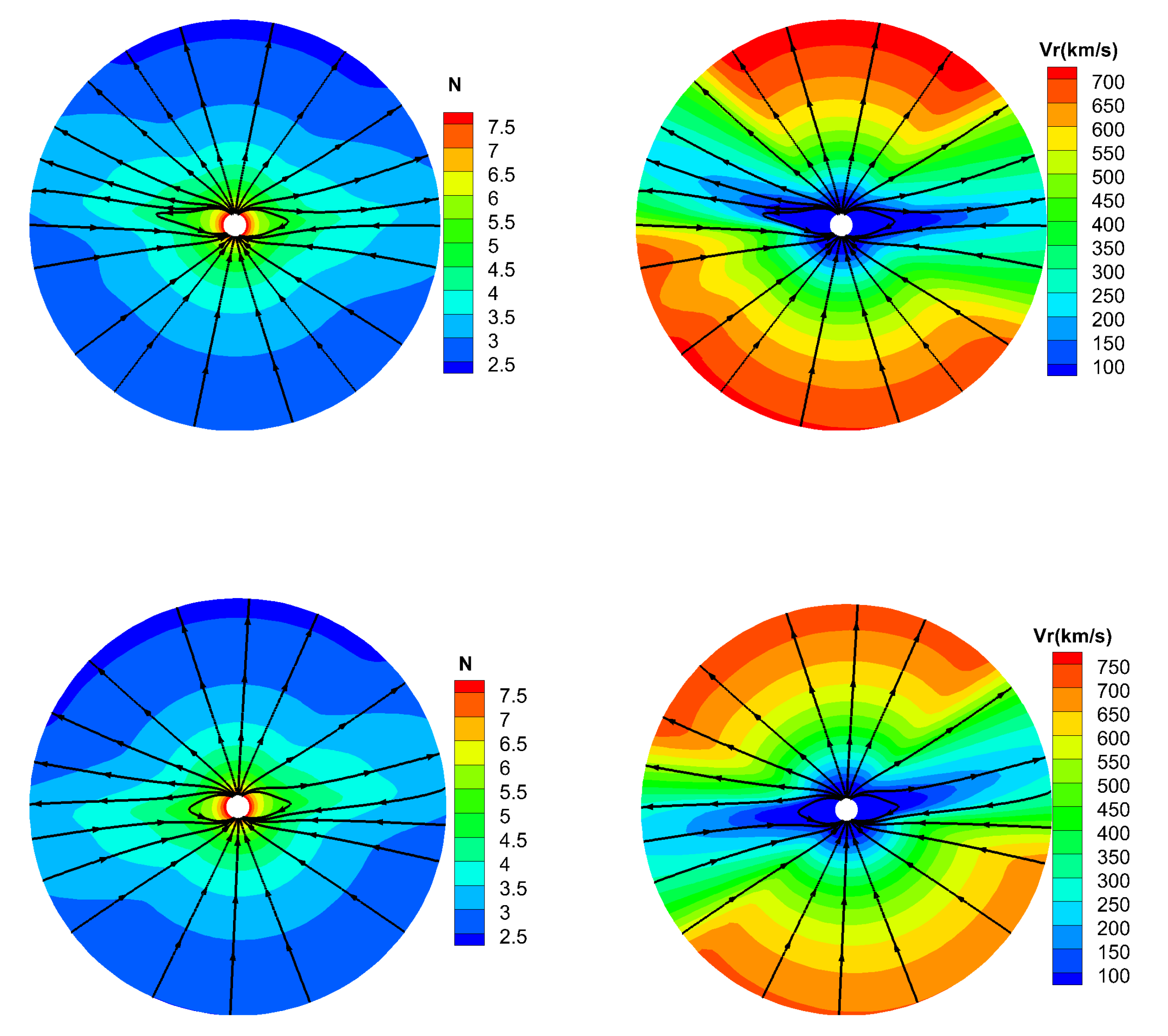
Figure 2 shows the model results for number density N, radial speed $v_r$ and the magnetic fields lines on meridional planes at $\varphi ={180}^{\circ }–0^{\circ }$ and $\varphi ={270}^{\circ }–{90}^{\circ }$ from 1–20 R${}_s$, where arrowheads on the black lines stand for the direction of magnetic fields. It can be seen from this figure that the fast solar wind flows and low density exist at the high latitudes, where the magnetic field lines extend to interplanetary space in this region. However, at lower latitudes around the vicinity of the equator or heliospheric current sheet (HCS) region showed the slow solar wind and high density, and a helmet streamer stretched by the solar wind can be observed within about five solar radii. Above the streamer, a thin current sheet is displayed between different magnetic polarities. These are the typical structures of solar wind in the solar minimum.

Figure 3 shows the coronal observations and simulated results on the meridional planes at $\varphi ={180}^{\circ }–0^{\circ }$ and $\varphi ={270}^{\circ }–{90}^{\circ }$. The first row displays the coronal pB images synthesized by the simulated results of the MHD model from 2.0 R${}_s$ to 6 R${}_s$. The second row shows the coronal pB images observed on August 14 (left) and August 5 (right) from the LASCO-C2 instrument on board the SOHO spacecraft. From this figure, we find that the positions of the bright structures are roughly matched in the observed and synthesized images. We infer that the bright structures are formed by streamers compared with the magnetic topologies in Figure 2.

Figure 4 presents the radial speed $v_r$ and Alfvénic surface (white line) on the meridional plane of $\varphi ={180}^{\circ }–0^{\circ }$ and $\varphi ={270}^{\circ }–{90}^{–}$ from 1–20 R${}_s$. Following [30], the Alfvénic surface is defined as $M_A=\frac{v\sqrt{\mu \rho }}{B}=1$. Since the solar wind is not spherical and smaller velocities exist at lower latitudes, the Alfvénic surface is wispy. In the inner corona below the Alfvénic surface, the magnetic stress dominates the interaction. The coronal magnetic field is largely dipole-like around the minimum phase of solar activity. The gradient of radial field strength in latitude, with stronger field at higher magnetic latitude, bends stream lines from the radial direction toward the magnetic equator. However, in the corona beyond the Alfvénic surface, it is the inertia of radially accelerated plasma flow that dominates the magnetic field-plasma interaction. The lowest Alfvénic surface occurs in the equator and the highest Alfvénic surface occurs in the pole [30,34,35]. Based on the radial evolution of the direction of coronal magnetic field, ref. [35] showed that the coronal helmet streamer belts observed at several heights by SOHO/LASCO, together with the source surface field of the horizontal current-current sheet-source surface model, can be used to find the heliocentric distance of the lowest and highest Alfvénic critical point. The highest Alfvénic critical point around the solar minimum is located between 10 and 14 solar radii. Similar to that in [30,35], the Alfvénic surface ranges from about 5 to 11 solar radii during this Carrington rotation.

To quantitatively see the divergence of magnetic fields, two types of divergence error are defined: $\mathrm{Error}1\left(\mathbf{B}\right)=\frac{\left|{\int }_{{\Omega }_k}\nabla ·\mathbf{B}dV\right|}{{\Omega }_k}$, $\mathrm{Error}2\left(\mathbf{B}\right)=\frac{\left|{\int }_{{\Omega }_k}\nabla ·\mathbf{B}dV\right|·\left|R\right|}{\left|{\int }_{{\Omega }_k}\mathbf{B}dV\right|}$ [28], where $R^2=3/\left(\frac{1}{{(\Delta r)}^2}+\frac{1}{{(r\Delta \theta )}^2}+\frac{1}{{(rsin\theta \Delta \varphi )}^2}\right)$ is the characteristic size of the cell. Additionally, the L1 normalization for divergence of magnetic fields $\mathrm{Norm}\left(\mathbf{B}\right)=\frac{\overline{\nabla ·\mathbf{B}}}{\parallel \overline{\nabla ·\mathbf{B}}\parallel }$ is defined, with $\parallel \parallel$ as the L1 norm. Figure 5 shows the initial profile of divergence on the meridional plane of $\varphi ={180}^{\circ }–0^{\circ }$. We can see that the divergence is about ${10}^{-10}\sim {10}^{-12}$, and the magnetic fields is divergence free under machine error. Since the CT method can maintain the initial divergence error unchanged in computation, the divergence error keep almost the same t = 20 h as initially, which can be seen from Figure 6.

Figure 7 shows the L1 normalization for divergence of magnetic fields on the meridional plane of $\varphi ={180}^{\circ }–0^{\circ }$ from 1 to 20 R${}_s$ at t = 20 h. The volume averaged divergence is about ${10}^{-10}$. The total number of cells in the computational domain is ${10}^6$, thus the L1 norm of the divergence $\parallel \overline{\nabla ·\mathbf{B}}\parallel$ is about ${10}^{-5}$. The normalization $\frac{\overline{\nabla ·\mathbf{B}}}{\parallel \overline{\nabla ·\mathbf{B}}\parallel }$ is about ${10}^{-5}$.

Figure 8 shows the evolution of the average divergence errors as a function of time. The average relative divergence errors are defined as $\mathrm{Error}1{\left(\mathbf{B}\right)}^{ave}={\sum }_{k=1}^M\frac{\left|{\int }_{{\Omega }_k}\nabla ·\mathbf{B}dV\right|}{{\Omega }_k}/M$, $\mathrm{Error}2{\left(\mathbf{B}\right)}^{ave}={\sum }_{k=1}^M\frac{\left|{\int }_{{\Omega }_k}\nabla ·\mathbf{B}dV\right|·\left|R\right|}{\left|{\int }_{{\Omega }_k}\mathbf{B}dV\right|}/M$, where M is the total number of cells in the computational domain. We can see that $\mathrm{Error}1{\left(\mathbf{B}\right)}^{ave}$ and $\mathrm{Error}2{\left(\mathbf{B}\right)}^{ave}$ are about ${10}^{-11}$ and ${10}^{-12}$, respectively. These divergence errors stay the same after 10 h and no obvious large error appears after a long run time. Thus, the magnetic field can be stated as divergence free during calculation.

Figure 9 presents the variation of number density N and radial speed $v_r$ from 1 R${}_s$ to 20 R${}_s$ at different latitudes, where $\theta =2^{\circ }$ corresponds to the open field region while $\theta ={90}^{\circ }$ corresponds to the HCS region. As usual, the fast solar wind exists in the open field region, whereas the slow solar wind exists in the HCS region, and the variation of number density is opposite to that of the speed.

Figure 10 displays the number density, radial speed and temperature maps for the MHD steady-state solution at 2.5 R${}_s$ and 20 R${}_s$. The left column denotes number density N with unit ${10}^6{\mathrm{cm}}^{-3},{10}^4{\mathrm{cm}}^{-3}$ from top to bottom, the middle column denotes radial speed $v_r$ with unit km/s, the last column denotes temperature T with unit ${10}^5$ K. Obviously, the number density decreases with radial distance while radial speed increases. The HCS region has high density, low speed and low temperature, whereas the inverse condition is seen at the polar or the open field region.

To further validate the simulated results, we map the in situ measurements at 1 au during CR 2207 at the OMNI website back to 20 $R_s$ by using a ballistic approximation [29]. Figure 11 shows the temporal profile of radial speed $v_r$ from the mapped observations (solid line) and the MHD model (dashed line). Although a deviation is exist at the first high-speed stream obtained by the MHD model, the simulated results roughly catch the second and third high-speed streams at about $\varphi ={200}^{\circ }$ and ${300}^{\circ }$.

5. Conclusions and Discussions

In this paper, a three-order, divergence-free finite volume scheme is introduced to simulate the steady state solar wind ambient. The CT method is used to maintain the divergence-free condition of the magnetic field. A least-squares reconstruction of the magnetic field with the divergence free constraints is used to make the magnetic fields global solenoidality initially. To achieve high order accuracy in space, a three order polynomial combined with the hierarchical non-oscillatory reconstruction in each cell is obtained. The three order Runge–Kutta scheme is used for time discretization. Additionally, the composite mesh with six-component grids proposed by [27,28,31] is used for parallelization in $(\theta ,\varphi )$ directions to reduce the computational cost.

The numerical results for Carrington rotation 2207 show its ability to produce stable reliable results for structured solar wind. For example, the slow speed solar wind exists near the slightly tilted helioshperic current sheet (HCS) plane and the fast speed solar wind exists near the poles. The magnetic field’s divergence error is around ${10}^{-12}$, which is around the machine round off error. All of these give us strong confidence in the current MHD code.

In the future, the propagation of coronal mass ejection in the solar-terrestrial space will be considered. To reach this goal it is first necessary to reconstruct the ambient background condition of solar wind, because these conditions will determine the evolution of coronal mass ejection. The domain will be extended to the Earth, and the propagation of the CME from Sun to Earth will be studied. To study the CME, as in the previous paper [30], a very simple spherical plasmoid model will be superposed on the background solar wind. The arrival time of the CME and Bz component, as well as the reconnection between CME and solar wind background will be investigated. Particularly, the resistive MHD will be used to study the reconnection between CME and solar wind; it is known that the electric resistivity term in the MHD is a second derivative term and its discretization will reduce the accuracy of the scheme, thus a high order is necessary. We believe that this new scheme can recover the reconnection process more accurately in the next work.

References

1. Feng, X. Magnetohydrodynamic Modeling of the Solar Corona and Heliosphere; Springer: Berlin/Heidelberg, Germany, 2020. [Google Scholar] [CrossRef]
2. Godunov, S.K. A difference method for numerical calculation of discontinuous solutions of the equations of hydrodynamics. Mat. Sb. Novaya Seriya 1959, 47, 271–306. [Google Scholar]
3. van Leer, B. Towards the ultimate conservative difference scheme. V. A second-order sequel to Godunov’s method. J. Comput. Phys. 1979, 32, 101–136. [Google Scholar] [CrossRef]
4. Woodward, P.; Colella, P. The numerical simulation of two-dimensional fluid flow with strong shocks. J. Comput. Phys. 1984, 54, 115–173. [Google Scholar] [CrossRef]
5. Shu, C.W. High Order Weighted Essentially Nonoscillatory Schemes for Convection Dominated Problems. SIAM Rev. 2009, 51, 82–126. [Google Scholar] [CrossRef] [Green Version]
6. Susanto, A.; Ivan, L.; Sterck, H.D.; Groth, C.P.T. High-order central ENO finite-volume scheme for ideal MHD. J. Comput. Phys. 2013, 250, 141–164. [Google Scholar]
7. Núñez-de la Rosa, J.; Munz, C.D. XTROEM-FV: A new code for computational astrophysics based on very high-order finite volume methods. Part I: Magnetohydrodynamics. Mon. Not. R. Astron. Soc. 2016, 460, 3458–3479. [Google Scholar] [CrossRef]
8. Felker, K.G.; Stone, J. A fourth-order accurate finite volume method for ideal MHD via upwind constrained transport. J. Comput. Phys. 2018, 375, 1365–1400. [Google Scholar] [CrossRef] [Green Version]
9. Du, Y.; Yuan, L.; Wang, Y. A High-Order Modified Finite Volume WENO Method on 3D Cartesian Grids. Commun. Comput. Phys. 2019, 26, 768–784. [Google Scholar] [CrossRef]
10. Harten, A.; Engquist, B.; Osher, S.; Chakravarthy, S.R. Uniformly High Order Accurate Essentially Non-Oscillatory Schemes 3. J. Comput. Phys. 1987, 71, 231–303. [Google Scholar] [CrossRef]
11. Liu, X.D.; Osher, S.; Chan, T. Weighted Essentially Non-Oscillatory Schemes. J. Comput. Phys. 1994, 115, 200–212. [Google Scholar] [CrossRef] [Green Version]
12. Jiang, G.S.; Shu, C.W. Efficient Implementation of Weighted ENO Schemes. J. Comput. Phys. 1996, 126, 202–228. [Google Scholar] [CrossRef] [Green Version]
13. Mignone, A. High-order conservative reconstruction schemes for finite volume methods in cylindrical and spherical coordinates. J. Comput. Phys. 2014, 270, 784–814. [Google Scholar] [CrossRef] [Green Version]
14. Colella, P.; Woodward, P.R. The Piecewise Parabolic Method (PPM) for gas-dynamical simulations. J. Comput. Phys. 1984, 54, 174–201. [Google Scholar] [CrossRef] [Green Version]
15. Cockburn, B.; Shu, C.W. TVB Runge–Kutta local projection discontinuous Galerkin finite element method for conservation laws. II. General framework. Math. Comput. 1989, 52, 411–435. [Google Scholar]
16. Cockburn, B.; Shu, C.W. The Runge–Kutta local projection P1 discontinuous Galerkin finite element method for scalar conservation laws. ESAIM Math. Model. Numer. Anal. 1991, 25, 337–361. [Google Scholar] [CrossRef]
17. Li, F.; Shu, C.W. Locally Divergence-Free Discontinuous Galerkin Methods for MHD Equations. J. Sci. Comput. 2005, 22, 413–442. [Google Scholar] [CrossRef]
18. Li, F.; Xu, L. Arbitrary order exactly divergence-free central discontinuous Galerkin methods for ideal MHD equations. J. Comput. Phys. 2012, 231, 2655–2675. [Google Scholar] [CrossRef]
19. Liu, Y.; Shu, C.W.; Tadmor, E.; Zhang, M. Non-Oscillatory Hierarchical Reconstruction for Central and Finite Volume Schemes. Commun. Comput. Phys. 2007, 2, 933–963. [Google Scholar]
20. Li, S. High order central scheme on overlapping cells for magneto-hydrodynamic flows with and without constrained transport method. J. Comput. Phys. 2008, 227, 7368–7393. [Google Scholar] [CrossRef]
21. Li, S. A fourth-order divergence-free method for MHD flows. J. Comput. Phys. 2010, 229, 7893–7910. [Google Scholar] [CrossRef]
22. Balsara, D.S. Self-adjusting, positivity preserving high order schemes for hydrodynamics and magnetohydrodynamics. J. Comput. Phys. 2012, 231, 7504–7517. [Google Scholar] [CrossRef]
23. Powell, K.G.; Roe, P.L.; Quirk, J. Adaptive-mesh algorithms for computational fluid dynamics. In Algorithmic Trends in Computational Fluid Dynamics; Springer: Berlin/Heidelberg, Germany, 1993; pp. 303–337. [Google Scholar]
24. Dedner, A.; Kemm, F.; Króner, D.; Munz, C.D.; Schnitzer, T.; Wesenberg, W. Hyperbolic divergence cleaning for the MHD equations. J. Comput. Phys. 2002, 175, 645–673. [Google Scholar] [CrossRef] [Green Version]
25. Feng, X.S.; Zhang, S.H.; Xiang, C.Q.; Yang, L.P.; Jiang, C.W.; Wu, S.T. A Hybrid Solar Wind Model of the CESE+HLL Method with a Yin-Yang Overset Grid and an AMR Grid. Astrophys. J. 2011, 734, 50. [Google Scholar] [CrossRef] [Green Version]
26. Shen, F.; Shen, C.L.; Zhang, J.; Hess, P.; Wang, Y.M.; Feng, X.S.; Cheng, H.Z.; Yang, Y. Evolution of the 12 July 2012 CME from the Sun to the Earth: Data-constrained three-dimensional MHD simulations. J. Geophys. Res. Space Phys. 2014, 119, 7128–7141. [Google Scholar] [CrossRef] [Green Version]
27. Feng, X.; Zhang, M.; Zhou, Y. A New Three-dimensional Solar Wind Model in Spherical Coordinates with a Six-component Grid. Astrophys. J. Suppl. Ser. 2014, 214, 6. [Google Scholar] [CrossRef] [Green Version]
28. Zhang, M.; Feng, X. A Comparative Study of Divergence Cleaning Methods of Magnetic Field in the Solar Coronal Numerical Simulation. Front. Astron. Space Sci. 2016, 3, 6. [Google Scholar] [CrossRef] [Green Version]
29. Feng, X.; Liu, X.J.; Xiang, C.; Li, H.C.; Wei, F. A New MHD Model with a Rotated-hybrid Scheme and Solenoidality-preserving Approach. Astrophys. J. 2019, 871, 226. [Google Scholar] [CrossRef]
30. Zhang, M.; Feng, X.; Liu, X.; Yang, L. A Provably Positive, Divergence-free Constrained Transport Scheme for the Simulation of Solar Wind. Astrophys. J. Suppl. Ser. 2021, 257, 32. [Google Scholar] [CrossRef]
31. Feng, X.; Yang, L.; Xiang, C.; Wu, S.T.; Zhou, Y.; Zhong, D. Three-dimensional solar wind modeling from the Sun to Earth by a SIP-CESE MHD model with a six-component grid. Astrophys. J. 2010, 723, 300–319. [Google Scholar] [CrossRef]
32. Shu, C. Total-Variation-Diminishing Time Discretizations. SIAM J. Sci. Stat. Comput. 1988, 9, 1073–1084. [Google Scholar] [CrossRef]
33. Parker, E.N. Interplanetary Dynamical Processes; Interscience Publishers: New York, NY, USA, 1963. [Google Scholar]
34. Pneuman, G.W.; Kopp, R.A. Gas-Magnetic Field Interactions in the Solar Corona. Sol. Phys. 1971, 18, 258–270. [Google Scholar] [CrossRef]
35. Zhao, X.P.; Hoeksema, J.T. The Magnetic Field at the Inner Boundary of the Heliosphere Around Solar Minimum. Sol. Phys. 2010, 266, 379–390. [Google Scholar] [CrossRef] [Green Version]
Figure 1. The six-component meshes on the sphere.
Universe 08 00371 g001
Figure 2. The model results for the magnetic field lines, radial speed v r (km/s), and number density N ( l o g 10 / cm 3 ) on the meridional plane of ϕ = 180 0 (top) and ϕ = 270 90 (bottom) from 1 to 20 R s .
Universe 08 00371 g002
Figure 3. Coronal polarized brightness images from 2.0 R s to 6 R s , and observed by LASCO C2/SOHO (bottom). The (left,right) panels of the top row are the views projected on the meridional planes with ϕ = 180 0 and ϕ = 270 90 , respectively. The (bottom) panels are the observations made on 14 August and 5 August 2018.
Universe 08 00371 g003
Figure 4. The model results for radial speed v r (km/s) and Alfvénic surface (white line) on the meridional plane of ϕ = 180 0 (left) and ϕ = 270 90 (right) from 1–20 R s .
Universe 08 00371 g004
Figure 5. The initial profile of Error 1 ( B ) (left) and Error 2 ( B ) (right) on the meridional plane of ϕ = 180 0 from 1 to 20 R s .
Universe 08 00371 g005
Figure 6. The profile of Error 1 ( B ) (left) and Error 2 ( B ) (right) on the meridional plane of ϕ = 180 0 from 1 to 20 R s at t = 20 h.
Universe 08 00371 g006
Figure 7. The L1 normalization for divergence of magnetic fields on the meridional plane of ϕ = 180 0 from 1 to 20 R s at t = 20 h.
Universe 08 00371 g007
Figure 8. The temporal evolution of the l o g 10 Error 1 ( B ) a v e and l o g 10 Error 2 ( B ) a v e in the calculation.
Universe 08 00371 g008
Figure 9. The number density N ( log 10 / cm 3 ) distribution (left) and radial speed v r (km/s) profiles (right) along heliocentric distance with different latitudes θ = 2 and θ = 90 .
Universe 08 00371 g009
Figure 10. The modeled results at 2.5 R s (top row) and 20 R s (bottom row). The left column denotes number density N with unit 10 6 cm 3 , 10 4 cm 3 from top to bottom, the middle column denotes radial speed v r with unit km/s, the last column denotes temperature T with unit 10 5 K.
Universe 08 00371 g010
Figure 11. Temporal profiles of radial speed v r with unit km/s from the mapped observations (solid line) and the MHD model (dashed line).
Universe 08 00371 g011
Publisher’s Note: MDPI stays neutral with regard to jurisdictional claims in published maps and institutional affiliations.