
Effect of Ephemeris on Pulsar Timing and Navigation Accuracy Based on X-ray Pulsar Navigation-I Data


Abstract
:1. Introduction
2. Effect of Ephemeris on Pulsar Timing
2.1. Effect on Time Scale Conversion
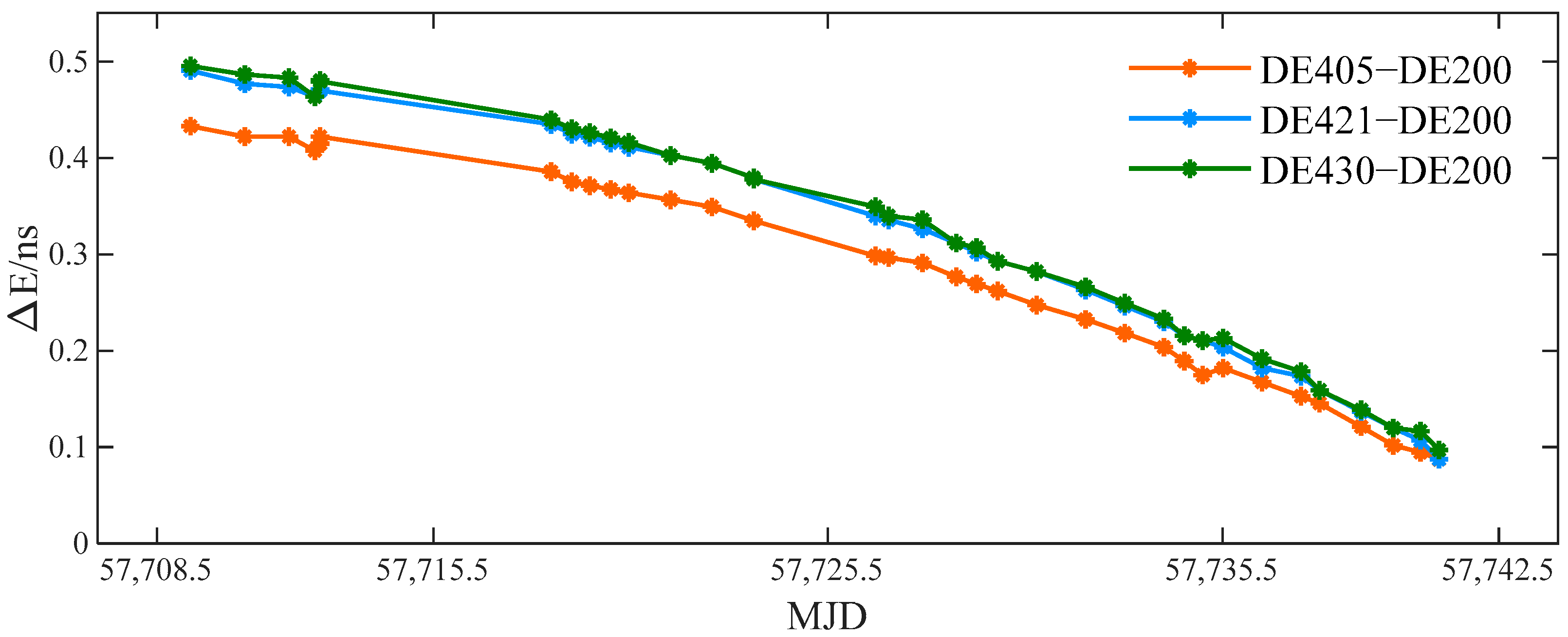
2.2. Effect on Light-Travel Delay
2.3. Comprehensive Impact Analysis on Timing Results
3. Effect of Ephemeris on Satellite Navigation and Orbit Determination
3.1. Positioning Error Modeling
3.2. Effect of Ephemeris on Single Pulsar Navigation or Orbit Determination
4. Experimental Results and Discussion
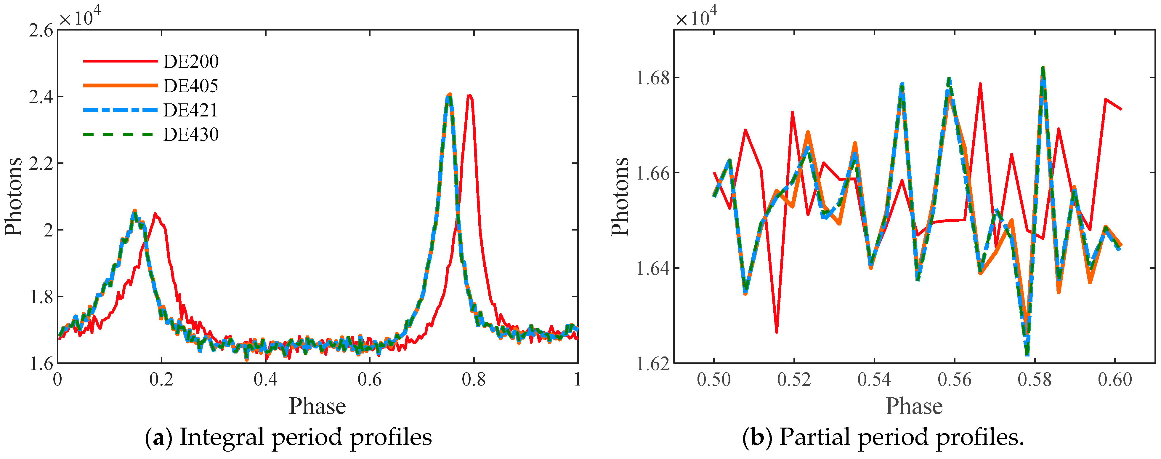
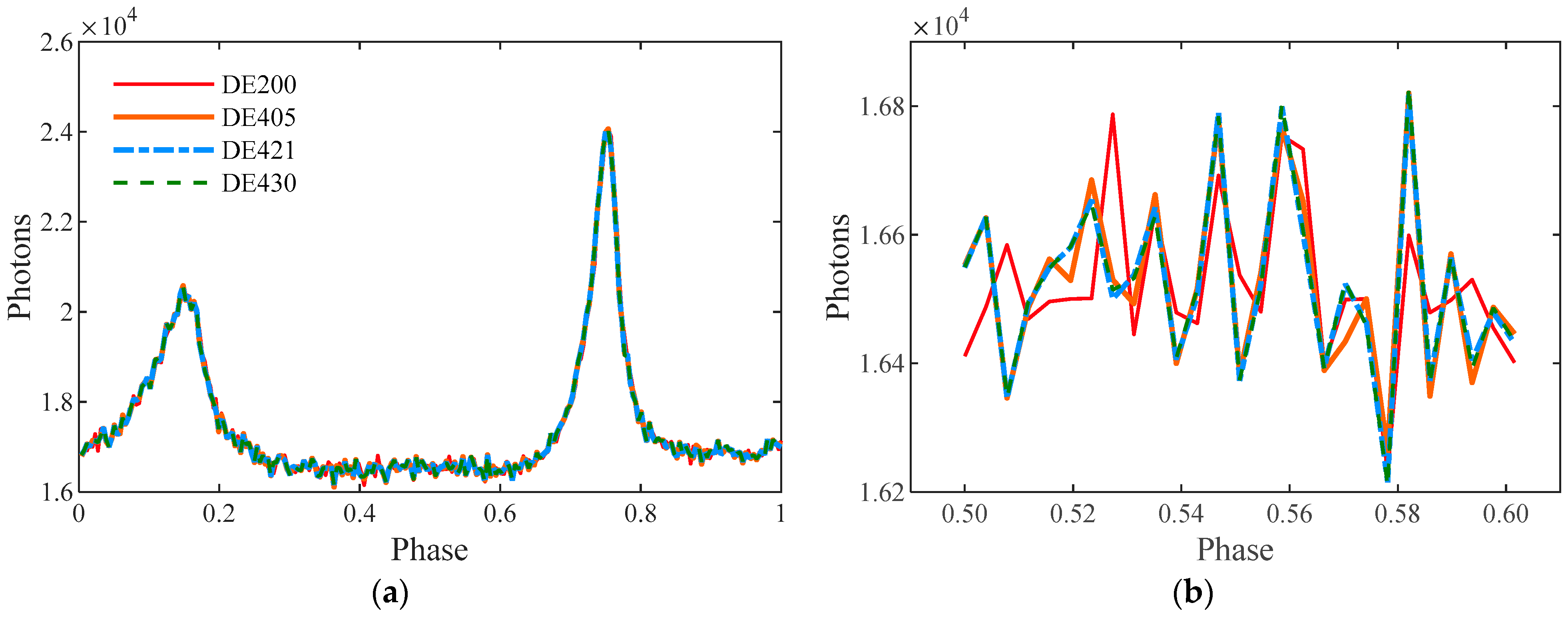
4.1. Pulse Profile
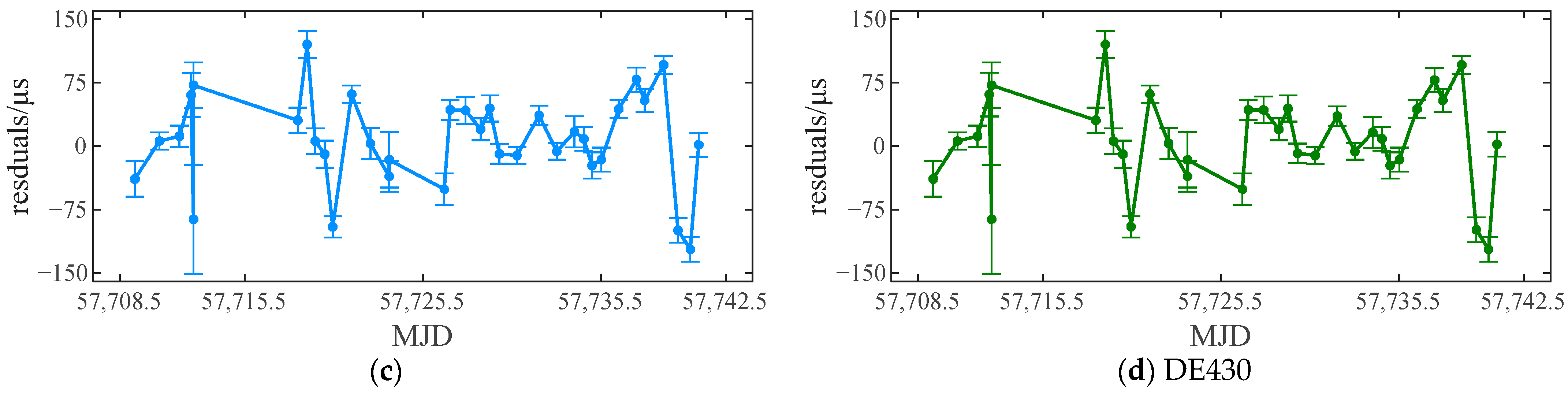
4.2. Timing Residuals
4.3. Orbit Determination Analysis
4.4. Discussion
5. Conclusions
Author Contributions
Funding
Institutional Review Board Statement
Informed Consent Statement
Data Availability Statement
Conflicts of Interest
Appendix A

| DE200 | DE405 | DE421 | DE430 | |
|---|---|---|---|---|
| Reference Frame | J2000.0 | ICRF | ICRF | ICRF2.0 |
| Time Span | JED2305424.5–JED 2513360.5 (AD1599–AD2169) | JED 2305424.5–JED2525008.5 (AD1599–AD2201) | JED 2414864.5–JED 2471184.5 (AD1899–AD2053) | JED2287184.5–JED2688976.5 (AD1549–AD2650) |
| Observation Data | Radar, Spacecraft | Radar, Spacecraft, CCD, RATE, Transit, Astrolabe | LLR, Radar, Spacecraft, CCD, Photo, Transit | LLR, Spacecraft, Radar, Astrometric, Occultation |
| Note | Including Nutation but excluding Libration | Including Nutation and Libration | Including Nutation and Libration | Including Nutation and Libration (1980 series) |
| Parameter | Value |
|---|---|
| Start time | UTC 2016/11/17(MJD:57,709.5) |
| End time | UTC 2016/12/19(MJD:57,741.5) |
| Number of observation orbits | 125 |
| Effective observation duration | 366,720 s |
| Number of detected photons | 4,438,661 counts |
| Source Flux | 1.0 counts/s |
| Background Flux | 14.2 counts/s |
| Timing Parameter | Value 1 | Value 2 |
|---|---|---|
| Right ascension (J2000) | 05 h 34 m 31.972 s | 05 h 34 m 31.972 s |
| Declination (J2000) | +22°00′52.07″ | +22°00′52.07″ |
| Reference epoch TDB | 2016/11/23 12:00:01.025488 MJD:57715.000000295 | 2016/12/16 12:00:01.0200448 MJD:57738.000000232 |
| Time range | 57,707~57,723 2016/11/15~12/01 | 57,723~57,754 2016/12/01~2017/01/01 |
| F0 [Hz] | 29.6478547478211 | 29.6471215546085 |
| F1 [Hz/s−1] | −3.68972−10 | −3.68942−10 |
| F2 [Hz/s−2] | −3.89−20 | 1.55−20 |
References
- Hewish, A.; Bell, S.J.; Pilkington, J.D.H.; Scott, P.F.; Collins, R.A. 74. Observation of a Rapidly Pulsating Radio Source. In A Source Book in Astronomy and Astrophysics, 1900–1975; Harvard University Press: Cambridge, MA, USA, 2013; pp. 498–504. [Google Scholar]
- Taylor, J.H. Pulsar timing and relativistic gravity. Philosophical Transactions of the Royal Society of London. Ser. A Phys. Eng. Sci. 1992, 341, 117–134. [Google Scholar]
- Ellis, J.; Lewicki, M. Cosmic String Interpretation of NANOGrav Pulsar Timing Data. Phys. Rev. Lett. 2021, 126, 041304. [Google Scholar] [CrossRef] [PubMed]
- Goncharov, B.; Shannon, R.; Reardon, D.; Hobbs, G.; Zic, A.; Bailes, M.; Curyło, M.; Dai, S.; Kerr, M.; Lower, M. On the evi-dence for a common-spectrum process in the search for the nanohertz gravitational-wave background with the Parkes Pulsar Timing Array. Astrophys. J. Lett. 2021, 917, L19. [Google Scholar] [CrossRef]
- Edwards, R.T.; Hobbs, G.; Manchester, R. TEMPO2, a new pulsar timing package–II. The timing model and precision estimates. Month. Not. R. Astr. Soc. 2006, 372, 1549–1574. [Google Scholar] [CrossRef] [Green Version]
- Verbiest, J.P.; Bailes, M.; van Straten, W.; Hobbs, G.B.; Edwards, R.T.; Manchester, R.N.; Bhat, N.; Sarkissian, J.M.; Jacoby, B.A.; Kulkarni, S.R. Precision timing of PSR J0437–4715: An accurate pulsar distance, a high pulsar mass, and a limit on the variation of Newton’s gravitational constant. Astrophys. J. 2008, 679, 675. [Google Scholar] [CrossRef]
- Huang, L.; Shuai, P.; Zhang, X.; Chen, S. A new explorer mission for soft X-ray timing—Observation of the Crab pulsar. Acta Astronaut. 2018, 151, 63–67. [Google Scholar] [CrossRef]
- Qing-Yong, Z.; Zi-Qing, W.; Lin-Li, Y.; Peng-Fei, S.; Si-Wei, L.; Lai-Ping, F.; Kun, J.; Yi-Di, W.; Yong-Xing, Z.; Xiao-Gang, L. Space/ground based pulsar timescale for comprehensive PNT system. Acta Phys. Sin. 2021, 70, 471–483. [Google Scholar]
- Downs, G. Interplanetary Navigation Using Pulsating Radio Sources; JPL Technical Report 32–1594; NASA: Washington, DC, USA, 1974. Available online: https://ntrs.nasa.gov/citations/19740026037 (accessed on 22 June 2022).
- Sheikh, S.I.; Pines, D.J.; Ray, P.S.; Wood, K.S.; Lovellette, M.N.; Wolff, M.T. Spacecraft Navigation Using X-Ray Pulsars. J. Guid. Control. Dyn. 2006, 29, 49–63. [Google Scholar] [CrossRef] [Green Version]
- Winternitz, L.B.; Hassouneh, M.A.; Mitchell, J.W.; Price, S.R.; Yu, W.H.; Semper, S.R.; Ray, P.S.; Wood, K.S.; Arzoumanian, Z.; Gendreau, K.C. SEXTANT X-ray Pulsar Navigation Demonstration: Additional On-Orbit Results. In Proceedings of the 2018 SpaceOps Conference, Marseille, France, 28 May–1 June 2018. [Google Scholar]
- Zhou, Q.; Ji, J.; Ren, H. The Timing Equation in X-Ray Pulsar Autonomous Navigation. In Proceedings of the China Satellite Navigation Conference (CSNC) 2013 Proceedings, Wuhan, China, 15–17 May 2013; pp. 543–554. [Google Scholar]
- Xu, Q.; Fan, X.; Ding, B.; Xu, L.; Liu, N. Adaptive two-stage Kalman filter for X-ray pulsar navigation. In Proceedings of the Seventh Symposium on Novel Photoelectronic Detection Technology and Applications, Kunming, China, 5–7 November 2021; p. 117635K. [Google Scholar]
- Xue, M.; Peng, D.; Sun, H.; Shentu, H.; Guo, Y.; Luo, J.; Zhikun, C. X-ray pulsar navigation based on two-stage estimation of Doppler frequency and phase delay. Aerosp. Sci. Technol. 2021, 110, 106470. [Google Scholar] [CrossRef]
- Ely, T.; Bhaskaran, S.; Bradley, N.; Lazio, T.J.W.; Martin-Mur, T. Comparison of Deep Space Navigation Using Optical Imaging, Pulsar Time-of-Arrival Tracking, and/or Radiometric Tracking. J. Astronaut. Sci. 2022, 69, 385–472. [Google Scholar] [CrossRef]
- Lv, Z.; Mei, Z.; Deng, L.; Li, L.; Chen, J. In-orbit calibration and data analysis of China’s first grazing incidence focusing X-ray pulsar telescope. Aerosp. China 2017, 18, 3–10. [Google Scholar]
- Huang, L.; Shuai, P.; Zhang, X.; Chen, S. Pulsar-based navigation results: Data processing of the X-ray pulsar navigation-I telescope. J. Astron. Telesc. Instr. Syst. 2019, 5, 018003. [Google Scholar] [CrossRef]
- Zheng, S.; Ge, M.; Han, D.; Wang, W.; Chen, Y.; Lu, F.; Bao, T.; Chai, J.; Dong, Y.; Feng, M.; et al. Test of pulsar navigation with POLAR on TG-2 space station. Sci. Sin. Phys. Mech. Astron. 2017, 47, 099505. [Google Scholar] [CrossRef] [Green Version]
- Zheng, S.; Zhang, S.; Lu, F.; Wang, W.; Gao, Y.; Li, T.; Song, L.; Ge, M.; Han, D.; Chen, Y. In-orbit demonstration of X-ray pulsar navigation with the Insight-HXMT satellite. Astrophys. J. Suppl. Ser. 2019, 244, 1. [Google Scholar] [CrossRef] [Green Version]
- Xue-Mei, D.; Min, F.; Yi, X. Comparisons and Evaluations of JPL Ephemerides. Chin. Astron. Astrophys. 2014, 38, 330–341. [Google Scholar] [CrossRef]
- JPL Planetary and Lunar Ephemerides. Available online: https://ssd.jpl.nasa.gov/planets/eph_export.html (accessed on 22 June 2021).
- Wang, Y.; Zheng, W.; Sun, S.; Li, L. X-ray pulsar-based navigation system with the errors in the planetary ephemerides for Earth-orbiting satellite. Adv. Space Res. 2013, 51, 2394–2404. [Google Scholar] [CrossRef]
- Xu, Q.; Wang, H.L.; You, S.; He, Y.Y.; Feng, L. Impact of Ephemeris Errors on X-ray Pulsar Navigation. In Proceedings of the 2018 IEEE CSAA Guidance, Navigation and Control Conference (CGNCC), Xiamen, China, 10–12 August 2018; pp. 1–6. [Google Scholar]
- Ning, X.; Yang, Y.; Li, Z.; Gui, M.; Fang, J. Ephemeris Corrections in Celestial/Pulsar Navigation Using Time Differential and Ephemeris Estimation. J. Guid. Control. Dyn. 2018, 41, 1–8. [Google Scholar] [CrossRef]
- Fang, H.; Su, J.; Li, L.; Zhang, L.; Sun, H.; Gao, J. An analysis of X-ray pulsar navigation accuracy in Earth orbit applications. Adv. Space Res. 2021, 68, 3731–3748. [Google Scholar] [CrossRef]
- Ge, M.Y.; Zhang, S.N.; Lu, F.; Li, T.P.; Yuan, J.P.; Zheng, X.P.; Huang, Y.; Zheng, S.J.; Chen, Y.P.; Chang, Z.; et al. Discovery of Delayed Spin-up Behavior Following Two Large Glitches in the Crab Pulsar, and the Statistics of Such Processes. Astrophys. J. Lett. 2020, 896, 55. [Google Scholar] [CrossRef]
- Kaplan, G.H. The IAU Resolutions on Astronomical Reference Systems, Time Scales, and Earth Rotation Models (Draft 4); Naval Observatory: Washington, DC, USA, 2005. [Google Scholar] [CrossRef] [Green Version]
- XPNAV-I Online Data. Available online: http://www.beidou.gov.cn/yw/xwzx/201710/t20171010_824.html (accessed on 22 June 2021).
- Petit, G.; Luzum, B. IERS Conventions (2010); Bureau International des Poids et Mesures Sevres: Saint-Cloud, France, 2010. [Google Scholar]
- Irwin, A.W.; Fukushima, T. A numerical time ephemeris of the Earth. Astron. Astrophys. 1999, 348, 642–652. [Google Scholar]
- Emadzadeh, A.A.; Speyer, J.L. On Modeling and Pulse Phase Estimation of X-Ray Pulsars. IEEE Trans. Signal Process. 2010, 58, 4484–4495. [Google Scholar] [CrossRef]
- Jodrell Bank Crab Pulsar Ephemeris. Available online: https://www.jb.man.ac.uk/pulsar/crab.html (accessed on 22 June 2021).
- The ATNF Pulsar Catalogue. Available online: https://www.atnf.csiro.au/research/pulsar/psrcat/ (accessed on 22 June 2021).
- Mao, Y.; Chen, J.; Song, X. Single X-ray pulsar dynamic orbit determination. J. Geom. Sci. Technol. 2010, 27, 251–254. [Google Scholar]
- Su, J.; Fang, H.; Bao, W.; Sun, H.; Shen, L.; Zhao, L. Fast simulation of X-ray pulsar signals at a spacecraft. Acta Astronaut. 2019, 166, 93–103. [Google Scholar] [CrossRef]


| UTC | TT | TCG | TCB | TDB | ΔE | |
|---|---|---|---|---|---|---|
| DE200 | 8:00:00 | 8:01:08.184 | 8:01:9.061046718583 | 8:01:27.695296538761 | 8:01:8.182794784679 | −0.0012052153210 |
| DE405 | 8:00:00 | 8:01:08.184 | TCGDE200 + 0.0 s | TCBDE200 + 4.47 × 10⁻¹⁰ s | TDBDE200 + 4.48 × 10⁻¹⁰ s | ΔEDE200 + 4.480 × 10⁻¹⁰ s |
| DE421 | 8:00:00 | 8:01:08.184 | TCGDE200 + 0.0 s | TCBDE200 + 5.06 × 10⁻¹⁰ s | TDBDE200 + 5.06 × 10⁻¹⁰ s | ΔEDE200 + 5.063 × 10⁻¹⁰ s |
| DE430 | 8:00:00 | 8:01:08.184 | TCGDE200 + 0.0 s | TCBDE200 + 5.13 × 10⁻¹⁰ s | TDBDE200 + 5.14 × 10⁻¹⁰ s | ΔEDE200 + 5.135 × 10⁻¹⁰ s |
| Roemer | Parallax | Shapiro | Light-Travel Delay | |
|---|---|---|---|---|
| DE200 | −433.639869983242 | 2.28207289 × 10⁻²⁷ | −2.59819521802 × 10⁻⁴ | −433.640129802764 |
| DE405 | ΔRDE200 + 1.355447560 × 10⁻³ | ΔPDE200 + 5.39 × 10⁻³² | ΔSDE200 − 6.60 × 10⁻¹³ | ΔLDE200 + 1.355447560 × 10⁻³ |
| DE421 | ΔRDE200 + 1.359091856 × 10⁻³ | ΔPDE200 + 5.39 × 10⁻³² | ΔSDE200 − 6.85 × 10⁻¹³ | ΔLDE200 + 1.359091856 × 10⁻³ |
| DE430 | ΔRDE200 + 1.358951972 × 10⁻³ | ΔPDE200 + 5.39 × 10⁻³² | ΔSDE200 − 6.91 × 10⁻¹³ | ΔLDE200 + 1.358951972 × 10⁻³ |
| Ephemerides | P_200_405 | P_200_421 | P_200_430 | P_405_421 | P_405_430 | P_421_430 |
| Pearson_corr | 0.996272152 | 0.996293838 | 0.996299275 | 0.999859096 | 0.999860405 | 0.999991201 |
| Ephemeris | DE200 | DE405 | DE421 | DE430 |
|---|---|---|---|---|
| RMSE | 54.6418 | 54.9246 | 54.5714 | 54.5273 |
| MAE | 44.4169 | 42.4389 | 42.1759 | 42.1400 |
| Ephemeris | DE405/200 | DE405/421 | DE421/430 |
|---|---|---|---|
| RMSE | 72.2760 | 54.5714 | 61.3338 |
| MAE | 57.6716 | 42.1759 | 45.9044 |
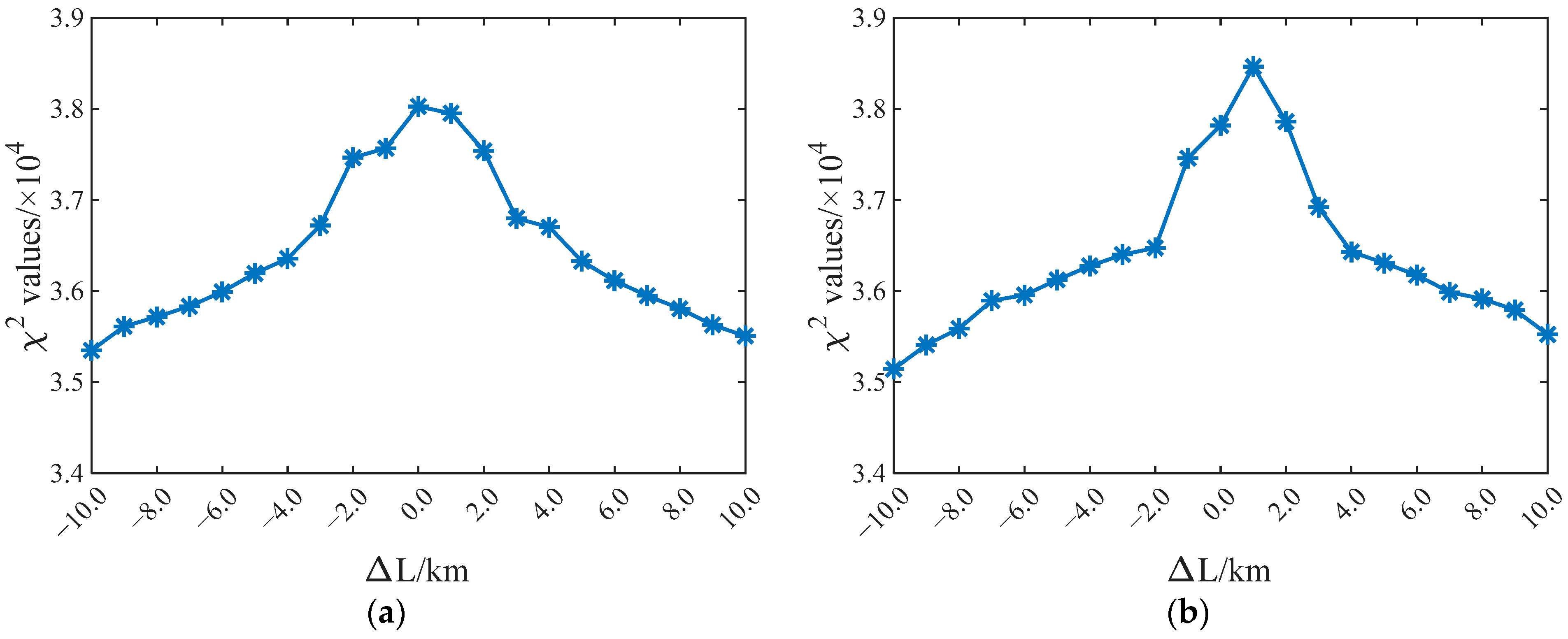
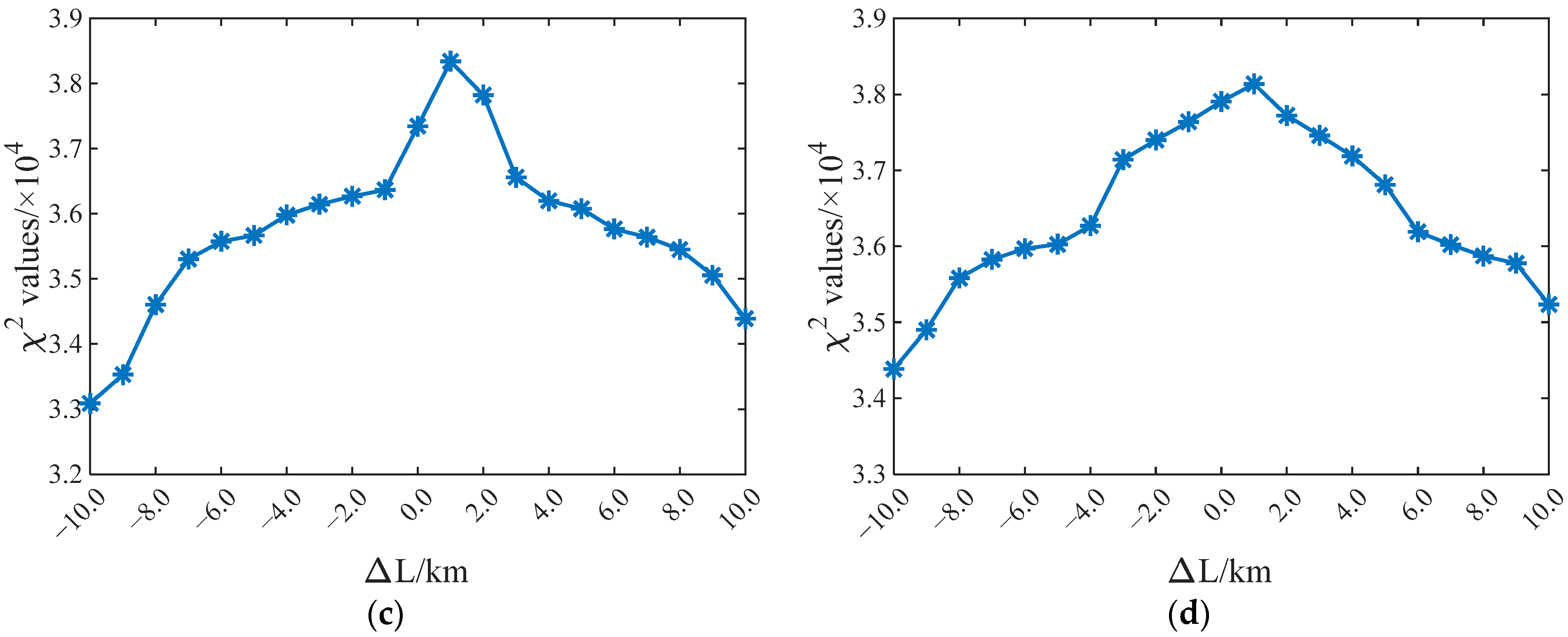
| ΔL/Km | DE200 | DE405 | DE421 | DE430 |
|---|---|---|---|---|
| −10 | 35,348.58282 | 35,144.58369 | 33,088.10955 | 34,385.1766 |
| −9 | 35,613.47329 | 35,409.82768 | 33,530.0139 | 34,900.42859 |
| −8 | 35,717.51518 | 35,589.39763 | 34,604.85721 | 35,581.71327 |
| −7 | 35,834.13222 | 35,895.86897 | 35,304.83125 | 35,826.32905 |
| −6 | 35,992.52258 | 35,956.87852 | 35,577.09967 | 35,970.18901 |
| −5 | 36,195.84801 | 36,124.38468 | 35,667.40987 | 36,026.41001 |
| −4 | 36,357.96755 | 36,276.69509 | 35,980.34176 | 36,271.05581 |
| −3 | 36,720.60294 | 36,402.48305 | 36,145.60529 | 37,140.7892 |
| −2 | 37,465.89581 | 36,474.49957 | 36,270.53755 | 37,401.09154 |
| −1 | 37,569.36244 | 37,460.36531 | 36,368.28404 | 37,639.15843 |
| 0 | 38,028.23266 | 37,819.99479 | 37,344.9412 | 37,907.62134 |
| 1 | 37,953.4562 | 38,466.26153 | 38,340.82654 | 38,138.94381 |
| 2 | 37,540.49097 | 37,862.25479 | 37,824.27274 | 37,723.94564 |
| 3 | 36,801.20982 | 36,922.62293 | 36,561.31364 | 37,458.42178 |
| 4 | 36,702.71458 | 36,431.87019 | 36,199.47831 | 37,187.3775 |
| 5 | 36,328.88002 | 36,310.29199 | 36,078.04842 | 36,811.37727 |
| 6 | 36,116.18036 | 36,176.77891 | 35,766.93906 | 36,192.90688 |
| 7 | 35,949.24826 | 35,989.3597 | 35,641.37276 | 36,021.83881 |
| 8 | 35,807.98256 | 35,915.39357 | 35,451.27367 | 35,873.25145 |
| 9 | 35,629.80379 | 35,793.25319 | 35,055.39206 | 35,776.89203 |
| 10 | 35,507.51493 | 35,524.15199 | 34,390.37655 | 35,235.99492 |
Publisher’s Note: MDPI stays neutral with regard to jurisdictional claims in published maps and institutional affiliations. |
© 2022 by the authors. Licensee MDPI, Basel, Switzerland. This article is an open access article distributed under the terms and conditions of the Creative Commons Attribution (CC BY) license (https://creativecommons.org/licenses/by/4.0/).
Share and Cite
Deng, Y.; Jin, S. Effect of Ephemeris on Pulsar Timing and Navigation Accuracy Based on X-ray Pulsar Navigation-I Data. Universe 2022, 8, 360. https://doi.org/10.3390/universe8070360
Deng Y, Jin S. Effect of Ephemeris on Pulsar Timing and Navigation Accuracy Based on X-ray Pulsar Navigation-I Data. Universe. 2022; 8(7):360. https://doi.org/10.3390/universe8070360
Chicago/Turabian StyleDeng, Yongtao, and Shuanggen Jin. 2022. "Effect of Ephemeris on Pulsar Timing and Navigation Accuracy Based on X-ray Pulsar Navigation-I Data" Universe 8, no. 7: 360. https://doi.org/10.3390/universe8070360
APA StyleDeng, Y., & Jin, S. (2022). Effect of Ephemeris on Pulsar Timing and Navigation Accuracy Based on X-ray Pulsar Navigation-I Data. Universe, 8(7), 360. https://doi.org/10.3390/universe8070360