
Probing the Interior of the Schwarzschild Black Hole Using Congruences: LQG vs. GUP


Abstract
1. Introduction
2. General Schwarzschild Interior and Congruences
2.1. Timelike Case
2.2. Null Case
3. Classical Schwarzschild Interior
3.1. Metric and Classical Hamiltonian
3.2. Dynamics, Expansion Scalar and Raychaudhuri Equation
3.2.1. Generic and
3.2.2. Classical Dynamics
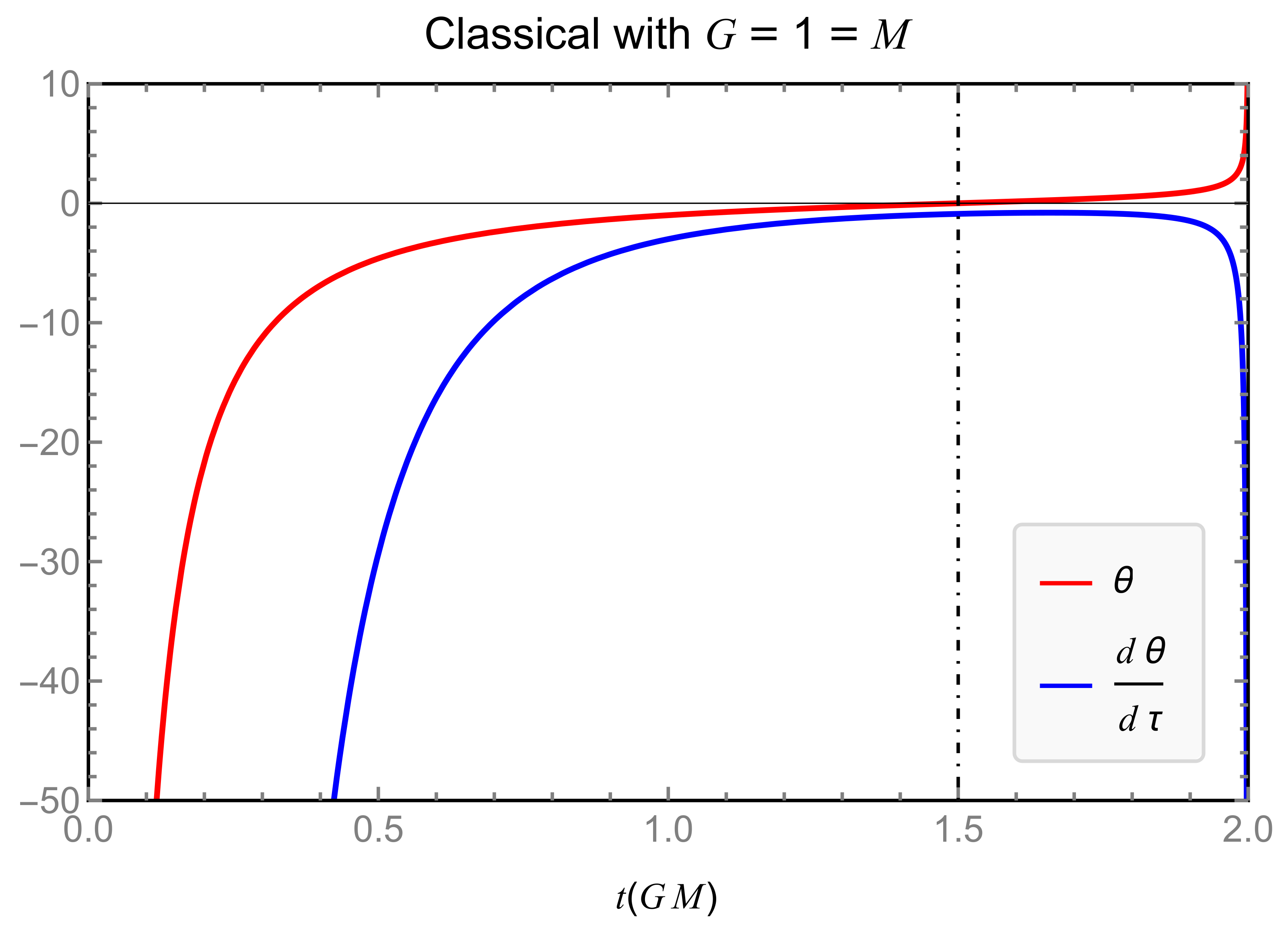
3.2.3. Classical and : Timelike Congruence
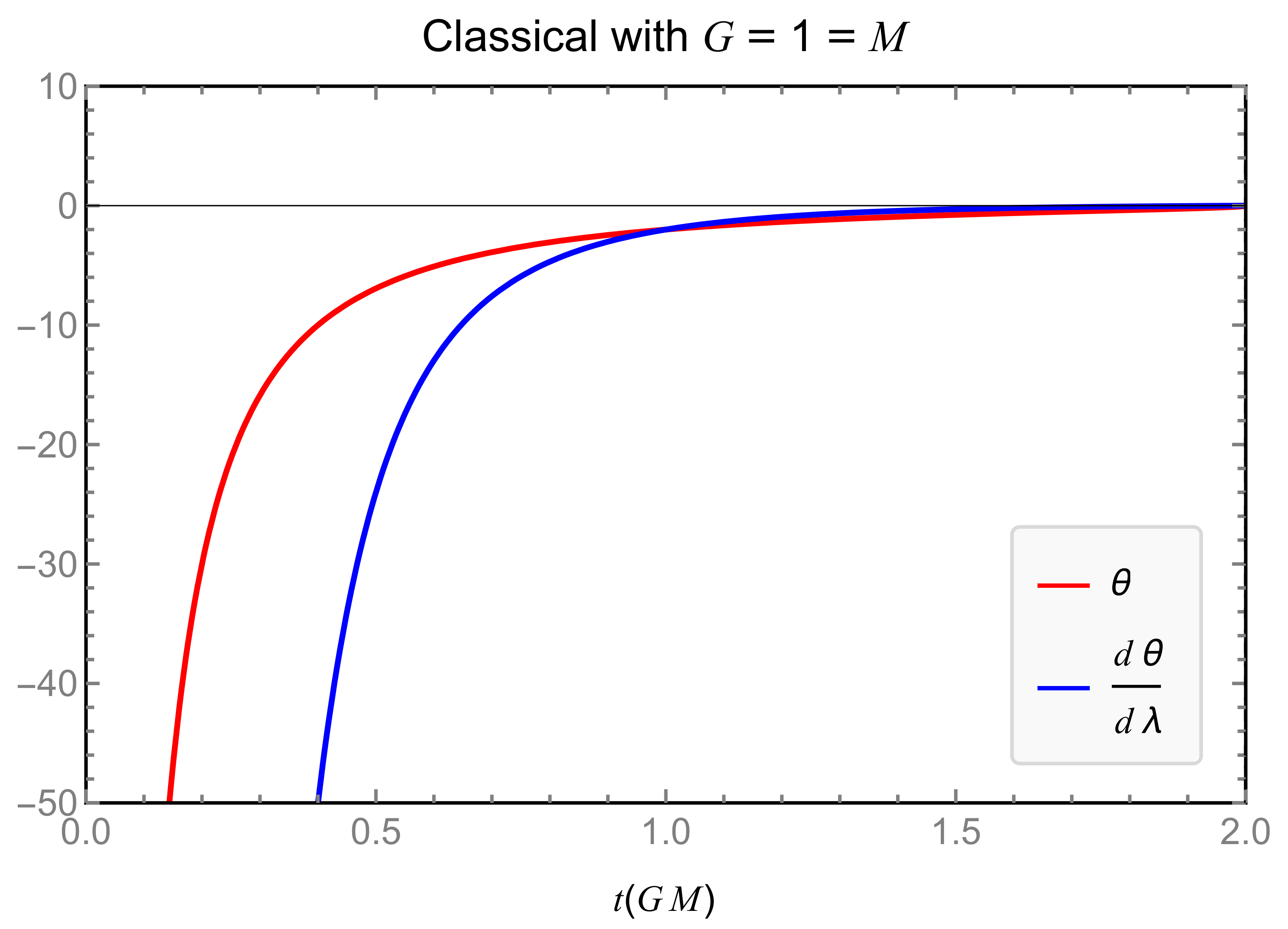
3.2.4. Classical and : Null Congruence
3.2.5. Classical Kretschmann Scalar
4. Effective Schwarzschild Interior
4.1. Loop Quantum Gravity
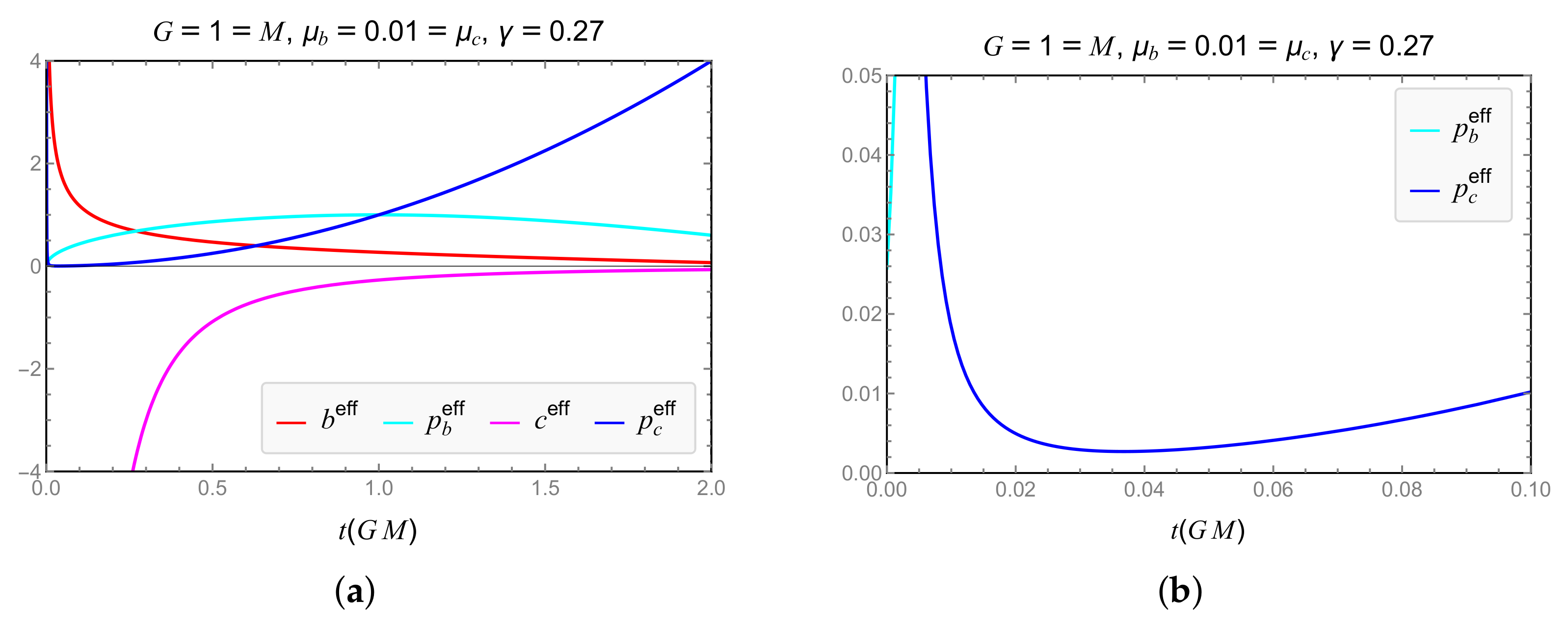
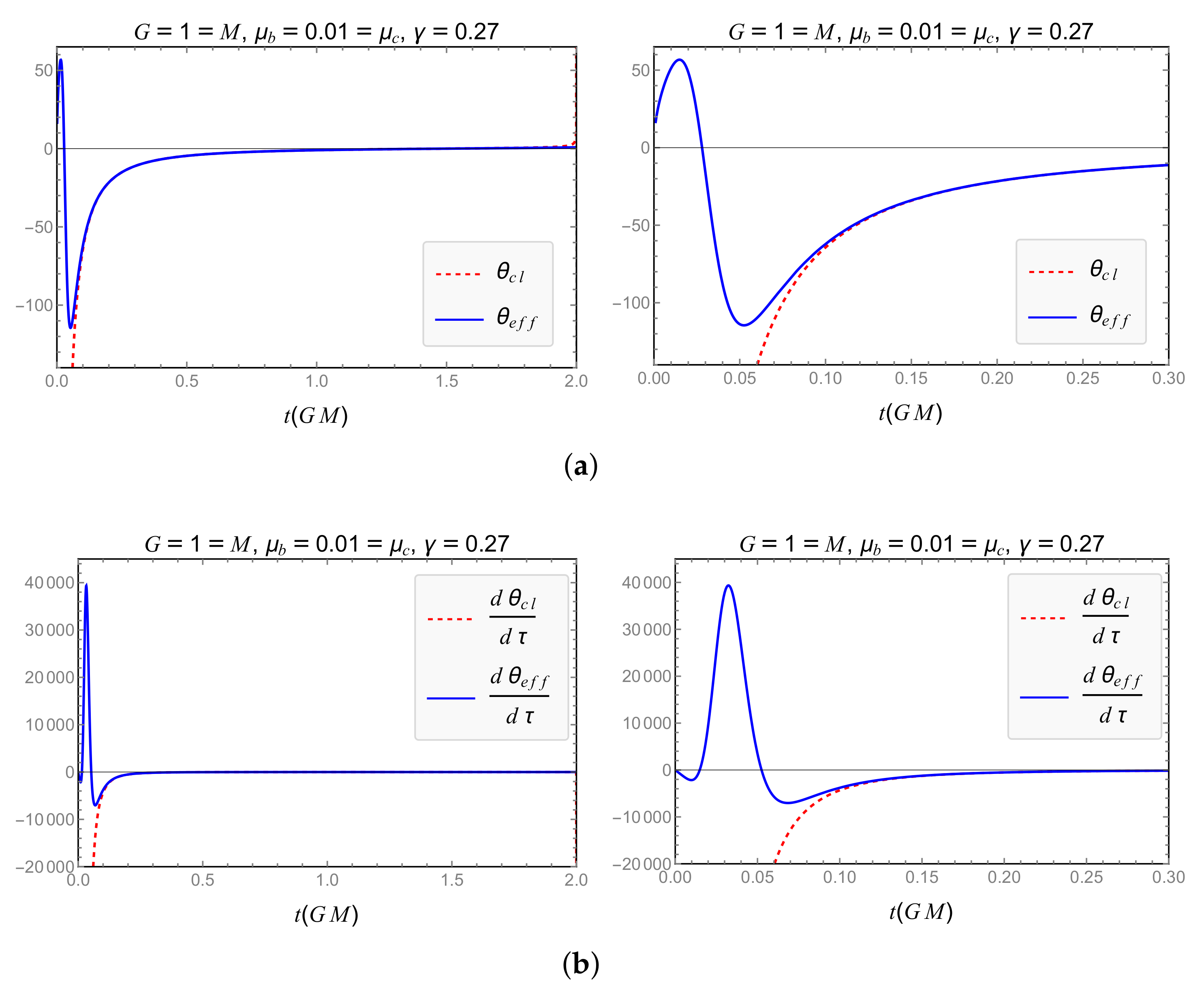
4.1.1. Scheme
4.1.2. Scheme
4.1.3. Scheme
4.2. Generalized Uncertainty Principle
5. Discussion
Author Contributions
Funding
Institutional Review Board Statement
Informed Consent Statement
Data Availability Statement
Conflicts of Interest
Abbreviations
| LQG | Loop quantum gravity |
| GUP | Generalized unicertaincty principle |
| EoM | Equations of motion |
| GR | General relativity |
| RE | Raychaudhuri equations |
Appendix A. Raychaudhuri Equation
Appendix A.1. Timelike Congruence
Appendix A.2. Null Congruence
| 1 | We use lower case Latin letter for abstract indices and Greek indices for components. |
References
- Thiemann, T. Modern Canonical Quantum General Relativity; Cambridge University Press: Cambridge, UK, 2007. [Google Scholar] [CrossRef]
- Ashtekar, A.; Bojowald, M. Quantum geometry and the Schwarzschild singularity. Class. Quant. Grav. 2006, 23, 391–411. [Google Scholar] [CrossRef]
- Bojowald, M. Spherically symmetric quantum geometry: States and basic operators. Class. Quant. Grav. 2004, 21, 3733–3753. [Google Scholar] [CrossRef]
- Bojowald, M.; Swiderski, R. Spherically symmetric quantum geometry: Hamiltonian constraint. Class. Quant. Grav. 2006, 23, 2129–2154. [Google Scholar] [CrossRef]
- Böhmer, C.G.; Vandersloot, K. Loop Quantum Dynamics of the Schwarzschild Interior. Phys. Rev. D 2007, 76, 104030. [Google Scholar] [CrossRef]
- Corichi, A.; Singh, P. Loop quantization of the Schwarzschild interior revisited. Class. Quant. Grav. 2016, 33, 055006. [Google Scholar] [CrossRef]
- Ashtekar, A.; Olmedo, J.; Singh, P. Quantum extension of the Kruskal spacetime. Phys. Rev. D 2018, 98, 126003. [Google Scholar] [CrossRef]
- Ben Achour, J.; Lamy, F.; Liu, H.; Noui, K. Polymer Schwarzschild black hole: An effective metric. Europhys. Lett. 2018, 123, 20006. [Google Scholar] [CrossRef]
- Bodendorfer, N.; Mele, F.M.; Münch, J. Effective Quantum Extended Spacetime of Polymer Schwarzschild Black Hole. Class. Quant. Grav. 2019, 36, 195015. [Google Scholar] [CrossRef]
- Bodendorfer, N.; Mele, F.M.; Münch, J. (b,v)-Type Variables for Black to White Hole Transitions in Effective Loop Quantum Gravity. 2019. Available online: https://arxiv.org/abs/1911.12646 (accessed on 1 May 2022).
- Bojowald, M.; Brahma, S.; Yeom, D.H. Effective line elements and black-hole models in canonical loop quantum gravity. Phys. Rev. D 2018, 98, 046015. [Google Scholar] [CrossRef]
- Campiglia, M.; Gambini, R.; Pullin, J. Loop quantization of spherically symmetric midi-superspaces: The Interior problem. AIP Conf. Proc. 2008, 977, 52–63. [Google Scholar] [CrossRef]
- Chiou, D.W. Phenomenological loop quantum geometry of the Schwarzschild black hole. Phys. Rev. D 2008, 78, 064040. [Google Scholar] [CrossRef]
- Corichi, A.; Karami, A.; Rastgoo, S.; Vukašinac, T. Constraint Lie algebra and local physical Hamiltonian for a generic 2D dilatonic model. Class. Quant. Grav. 2016, 33, 035011. [Google Scholar] [CrossRef]
- Cortez, J.; Cuervo, W.; Morales-Técotl, H.A.; Ruelas, J.C. Effective loop quantum geometry of Schwarzschild interior. Phys. Rev. D 2017, 95, 064041. [Google Scholar] [CrossRef]
- Gambini, R.; Pullin, J. Black holes in loop quantum gravity: The Complete space-time. Phys. Rev. Lett. 2008, 101, 161301. [Google Scholar] [CrossRef]
- Gambini, R.; Pullin, J.; Rastgoo, S. Quantum scalar field in quantum gravity: The vacuum in the spherically symmetric case. Class. Quant. Grav. 2009, 26, 215011. [Google Scholar] [CrossRef]
- Gambini, R.; Pullin, J.; Rastgoo, S. Quantum scalar field in quantum gravity: The propagator and Lorentz invariance in the spherically symmetric case. Gen. Rel. Grav. 2011, 43, 3569–3592. [Google Scholar] [CrossRef][Green Version]
- Gambini, R.; Pullin, J. Loop quantization of the Schwarzschild black hole. Phys. Rev. Lett. 2013, 110, 211301. [Google Scholar] [CrossRef]
- Gambini, R.; Olmedo, J.; Pullin, J. Spherically symmetric loop quantum gravity: Analysis of improved dynamics. Class. Quant. Grav. 2020, 37, 205012. [Google Scholar] [CrossRef]
- Husain, V.; Winkler, O. Quantum resolution of black hole singularities. Class. Quant. Grav. 2005, 22, L127–L134. [Google Scholar] [CrossRef]
- Husain, V.; Winkler, O. Quantum Hamiltonian for gravitational collapse. Phys. Rev. D 2006, 73, 124007. [Google Scholar] [CrossRef]
- Kelly, J.G.; Santacruz, R.; Wilson-Ewing, E. Effective Loop Quantum Gravity Framework for Vacuum Spherically Symmetric Space-Times. 2020. Available online: https://arxiv.org/abs/2006.09302 (accessed on 1 May 2022).
- Modesto, L. Loop quantum black hole. Class. Quant. Grav. 2006, 23, 5587–5602. [Google Scholar] [CrossRef]
- Modesto, L.; Premont-Schwarz, I. Self-dual Black Holes in LQG: Theory and Phenomenology. Phys. Rev. D 2009, 80, 064041. [Google Scholar] [CrossRef]
- Olmedo, J.; Saini, S.; Singh, P. From black holes to white holes: A quantum gravitational, symmetric bounce. Class. Quant. Grav. 2017, 34, 225011. [Google Scholar] [CrossRef]
- Thiemann, T.; Kastrup, H. Canonical quantization of spherically symmetric gravity in Ashtekar’s selfdual representation. Nucl. Phys. B 1993, 399, 211–258. [Google Scholar] [CrossRef]
- Zhang, C.; Ma, Y.; Song, S.; Zhang, X. Loop quantum Schwarzschild interior and black hole remnant. Phys. Rev. D 2020, 102, 041502. [Google Scholar] [CrossRef]
- Ziprick, J.; Gegenberg, J.; Kunstatter, G. Polymer Quantization of a Self-Gravitating Thin Shell. Phys. Rev. D 2016, 94, 104076. [Google Scholar] [CrossRef]
- Campiglia, M.; Gambini, R.; Pullin, J. Loop quantization of spherically symmetric midi-superspaces. Class. Quant. Grav. 2007, 24, 3649–3672. [Google Scholar] [CrossRef]
- Gambini, R.; Pullin, J.; Rastgoo, S. New variables for 1+1 dimensional gravity. Class. Quant. Grav. 2010, 27, 025002. [Google Scholar] [CrossRef]
- Rastgoo, S. A local true Hamiltonian for the CGHS Model in New Variables. 2013. Available online: https://arxiv.org/abs/1304.7836 (accessed on 1 May 2022).
- Corichi, A.; Olmedo, J.; Rastgoo, S. Callan-Giddings-Harvey-Strominger vacuum in loop quantum gravity and singularity resolution. Phys. Rev. D 2016, 94, 084050. [Google Scholar] [CrossRef]
- Morales-Técotl, H.A.; Rastgoo, S.; Ruelas, J.C. Effective dynamics of the Schwarzschild black hole interior with inverse triad corrections. Annals. Phys. 2021, 426, 168401. [Google Scholar] [CrossRef]
- Ben Achour, J.; Brahma, S.; Uzan, J.P. Bouncing compact objects. Part I. Quantum extension of the Oppenheimer-Snyder collapse. J. Cosmol. Astropart. Phys. 2020, 3, 41. [Google Scholar] [CrossRef]
- Blanchette, K.; Das, S.; Hergott, S.; Rastgoo, S. Black Hole Singularity Resolution via the Modified Raychaudhuri Equation in Loop Quantum Gravity. Phys. Rev. D 2021, 103, 084038. [Google Scholar] [CrossRef]
- Husain, V.; Kelly, J.G.; Santacruz, R.; Wilson-Ewing, E. On the Fate of Quantum Black Holes. 2022. Available online: https://arxiv.org/abs/2203.04238 (accessed on 1 May 2022).
- Addazi, A.; Alvarez-Muniz, J.; Batista, R.A.; Amelino-Camelia, G.; Antonelli, V.; Arzano, M.; Asorey, M.; Atteia, J.L.; Bahamonde, S.; Bajardi, F. Quantum gravity phenomenology at the dawn of the multi-messenger era—A review. Prog. Part. Nucl. Phys. 2021, 125, 103948. [Google Scholar] [CrossRef]
- Assanioussi, M.; Mickel, L. Loop effective model for Schwarzschild black hole interior: A modified dynamics. Phys. Rev. D 2021, 103, 124008. [Google Scholar] [CrossRef]
- Husain, V.; Kelly, J.G.; Santacruz, R.; Wilson-Ewing, E. Quantum Gravity of Dust Collapse: Shock Waves from Black Holes. Phys. Rev. Lett. 2022, 128, 121301. [Google Scholar] [CrossRef]
- Assanioussi, M.; Dapor, A.; Liegener, K. Perspectives on the dynamics in a loop quantum gravity effective description of black hole interiors. Phys. Rev. D 2020, 101, 026002. [Google Scholar] [CrossRef]
- Ashtekar, A.; Fairhurst, S.; Willis, J.L. Quantum gravity, shadow states, and quantum mechanics. Class. Quant. Grav. 2003, 20, 1031–1062. [Google Scholar] [CrossRef]
- Corichi, A.; Vukasinac, T.; Zapata, J.A. Polymer Quantum Mechanics and its Continuum Limit. Phys. Rev. D 2007, 76, 044016. [Google Scholar] [CrossRef]
- Morales-Técotl, H.A.; Rastgoo, S.; Ruelas, J.C. Path integral polymer propagator of relativistic and nonrelativistic particles. Phys. Rev. D 2017, 95, 065026. [Google Scholar] [CrossRef]
- Morales-Técotl, H.A.; Orozco-Borunda, D.H.; Rastgoo, S. Polymer quantization and the saddle point approximation of partition functions. Phys. Rev. D 2015, 92, 104029. [Google Scholar] [CrossRef]
- Flores-González, E.; Morales-Técotl, H.A.; Reyes, J.D. Propagators in Polymer Quantum Mechanics. Ann. Phys. 2013, 336, 394–412. [Google Scholar] [CrossRef]
- Ashtekar, A.; Pawlowski, T.; Singh, P. Quantum nature of the big bang. Phys. Rev. Lett. 2006, 96, 141301. [Google Scholar] [CrossRef]
- Ashtekar, A.; Pawlowski, T.; Singh, P. Quantum Nature of the Big Bang: An Analytical and Numerical Investigation. I. Phys. Rev. D 2006, 73, 124038. [Google Scholar] [CrossRef]
- Joe, A.; Singh, P. Kantowski-Sachs spacetime in loop quantum cosmology: Bounds on expansion and shear scalars and the viability of quantization prescriptions. Class. Quant. Grav. 2015, 32, 015009. [Google Scholar] [CrossRef]
- Saini, S.; Singh, P. Geodesic completeness and the lack of strong singularities in effective loop quantum Kantowski–Sachs spacetime. Class. Quant. Grav. 2016, 33, 245019. [Google Scholar] [CrossRef]
- Alesci, E.; Bahrami, S.; Pranzetti, D. Quantum gravity predictions for black hole interior geometry. Phys. Lett. B 2019, 797, 134908. [Google Scholar] [CrossRef]
- Alesci, E.; Bahrami, S.; Pranzetti, D. Asymptotically de Sitter universe inside a Schwarzschild black hole. Phys. Rev. D 2020, 102, 066010. [Google Scholar] [CrossRef]
- Das, S.; Vagenas, E.C. Universality of Quantum Gravity Corrections. Phys. Rev. Lett. 2008, 101, 221301. [Google Scholar] [CrossRef] [PubMed]
- Ali, A.F.; Das, S.; Vagenas, E.C. A proposal for testing Quantum Gravity in the lab. Phys. Rev. D 2011, 84, 044013. [Google Scholar] [CrossRef]
- Blanchette, K.; Das, S.; Rastgoo, S. Effective GUP-modified Raychaudhuri equation and black hole singularity: Four models. J. High Energy Phys. 2021, 09, 062. [Google Scholar] [CrossRef]
- Bosso, P.; Obregón, O.; Rastgoo, S.; Yupanqui, W. Deformed Algebra and the Effective Dynamics of the Interior of Black. 2020. Available online: https://arxiv.org/abs/2012.04795 (accessed on 1 May 2022).
- Villalpando, C.; Modak, S.K. Indirect Probe of Quantum Gravity using Molecular Wave-packets. Class. Quant. Grav. 2019, 36, 215016. [Google Scholar] [CrossRef]
- Das, S.; Fridman, M.; Lambiase, G.; Vagenas, E.C. Baryon asymmetry from the generalized uncertainty principle. Phys. Lett. B 2022, 824, 136841. [Google Scholar] [CrossRef]
- Mignemi, S. Extended uncertainty principle and the geometry of (anti)-de Sitter space. Mod. Phys. Lett. A 2010, 25, 1697–1703. [Google Scholar] [CrossRef]
- Costa Filho, R.N.; Braga, J.a.P.M.; Lira, J.H.S.; Andrade, J.S. Extended uncertainty from first principles. Phys. Lett. B 2016, 755, 367–370. [Google Scholar] [CrossRef]
- Schürmann, T. On the uncertainty principle in Rindler and Friedmann spacetimes. Eur. Phys. J. C 2020, 80, 141. [Google Scholar] [CrossRef]
- Dabrowski, M.P.; Wagner, F. Extended Uncertainty Principle for Rindler and cosmological horizons. Eur. Phys. J. C 2019, 79, 716. [Google Scholar] [CrossRef]
- Hamil, B.; Merad, M.; Birkandan, T. Applications of the extended uncertainty principle in AdS and dS spaces. Eur. Phys. J. Plus 2019, 134, 278. [Google Scholar] [CrossRef]
- Giné, J.; Luciano, G.G. Modified inertia from extended uncertainty principle(s) and its relation to MoND. Eur. Phys. J. C 2020, 80, 1039. [Google Scholar] [CrossRef]
- Wagner, F. Relativistic extended uncertainty principle from spacetime curvature. Phys. Rev. D 2022, 105, 025005. [Google Scholar] [CrossRef]
- Blanchette, K.; Das, S.; Hergott, S.; Rastgoo, S. Effective black hole interior and the Raychadhuri equation. In Proceedings of the 16th Marcel Grossmann Meeting on Recent Developments in Theoretical and Experimental General Relativity, Astrophysics and Relativistic Field Theories, Online, Italy, 5–9 July 2021; Available online: https://arxiv.org/abs/2110.05397 (accessed on 1 May 2022).
- Collins, C. Global structure of the Kantowski-Sachs cosmological models. J. Math. Phys. 1977, 18, 2116. [Google Scholar] [CrossRef]
- Chiou, D.W. Phenomenological dynamics of loop quantum cosmology in Kantowski-Sachs spacetime. Phys. Rev. D 2008, 78, 044019. [Google Scholar] [CrossRef]
- Morales-Técotl, H.A.; Orozco-Borunda, D.H.; Rastgoo, S. Polymerization, the Problem of Access to the Saddle Point Approximation, and Thermodynamics. In Proceedings of the 14th Marcel Grossmann Meeting on Recent Developments in Theoretical and Experimental General Relativity, Astrophysics, and Relativistic Field Theories, Rome, Italy, 12–18 July 2017; Volume 4, pp. 4054–4059. [Google Scholar]
- Modesto, L. Semiclassical loop quantum black hole. Int. J. Theor. Phys. 2010, 49, 1649–1683. [Google Scholar] [CrossRef]
- Ashtekar, A.; Pawlowski, T.; Singh, P. Quantum Nature of the Big Bang: Improved dynamics. Phys. Rev. D 2006, 74, 084003. [Google Scholar] [CrossRef]
- Ashtekar, A.; Wilson-Ewing, E. Loop quantum cosmology of Bianchi I models. Phys. Rev. D 2009, 79, 083535. [Google Scholar] [CrossRef]


| Model | Dependence of GUP Modifications on | Expansion and RE Finite for |
|---|---|---|
| 1 | Configuration | and |
| 2 | Momenta | No values of and |
| 3 | Configuration | and |
| 4 | Momenta | No values of and |
Publisher’s Note: MDPI stays neutral with regard to jurisdictional claims in published maps and institutional affiliations. |
© 2022 by the authors. Licensee MDPI, Basel, Switzerland. This article is an open access article distributed under the terms and conditions of the Creative Commons Attribution (CC BY) license (https://creativecommons.org/licenses/by/4.0/).
Share and Cite
Rastgoo, S.; Das, S. Probing the Interior of the Schwarzschild Black Hole Using Congruences: LQG vs. GUP. Universe 2022, 8, 349. https://doi.org/10.3390/universe8070349
Rastgoo S, Das S. Probing the Interior of the Schwarzschild Black Hole Using Congruences: LQG vs. GUP. Universe. 2022; 8(7):349. https://doi.org/10.3390/universe8070349
Chicago/Turabian StyleRastgoo, Saeed, and Saurya Das. 2022. "Probing the Interior of the Schwarzschild Black Hole Using Congruences: LQG vs. GUP" Universe 8, no. 7: 349. https://doi.org/10.3390/universe8070349
APA StyleRastgoo, S., & Das, S. (2022). Probing the Interior of the Schwarzschild Black Hole Using Congruences: LQG vs. GUP. Universe, 8(7), 349. https://doi.org/10.3390/universe8070349