1. Introduction
Gamma-ray bursts (GRBs) outshine their host galaxies, making them ideal candidates for probing large-scale structure, as they can be detected up to very high redshifts [
1,
2,
3,
4,
5,
6]. According to the Cosmological Principle, the Universe is spatially homogeneous and isotropic on a large scale: assuming that GRBs follow the distribution of baryonic matter, we would expect homogeneity and isotropy for GRBs as well. Hence, the spatial distribution of the GRBs allows us to test matter’s distribution in the Universe.
The paper is organized as follows:
Section 2 describes our dataset;
Section 3 overviews the previous statistical analyses and results regarding the GRBs’ distribution. In
Section 4, we determine the Sky Exposure Function for the GRBs with spectroscopic redshift. In
Section 5, the Spatial Two-Point Correlation Function is approximated, while
Section 6 discusses the results, and
Section 7 summarizes.
2. Data Selection
The sample of GRBs with measured position, optical afterglow, and spectroscopic redshift is created largely of bursts detected by NASA’s Swift and Fermi experiment. Here, we used the same dataset of Horvath et al. [
7], which used redshifts from the GRBOX database (Gamma-Ray Burst Online Index) database (the datasets were derived from different sources in the public domain:
https://www.astro.caltech.edu/grbox/grbox.php, (accessed on 4 June 2021)). The GRBOX database is heavily based on the notes of the Gamma-ray Coordination Network (
http://gcn.gsfc.nasa.gov/, (accessed on 4 June 2021)) and on the public dataset of Joachim Greiner (
http://www.mpe.mpg.de/~jcg/grbgen.html, (accessed on 4 June 2021)), which also contains much information about almost every GRB observed by any instrument.
The GRBOX catalog database (published by the Caltech Astronomy Department) has been carefully reviewed by its creators to avoid observations with large systematic uncertainties. The redshift data in Horvath et al. [
7] contain spectroscopic redshifts only. Photometric redshifts, as well as redshift estimations based on Ly-
limits are excluded as they introduce large (typically more than several hundreds of Mpc) radial distance uncertainties. By November 2013, the redshifts of 361 GRBs had been determined, and as of March 2018, the redshifts of 487 GRBs have been measured. Here, we expand the data of Horvath et al. [
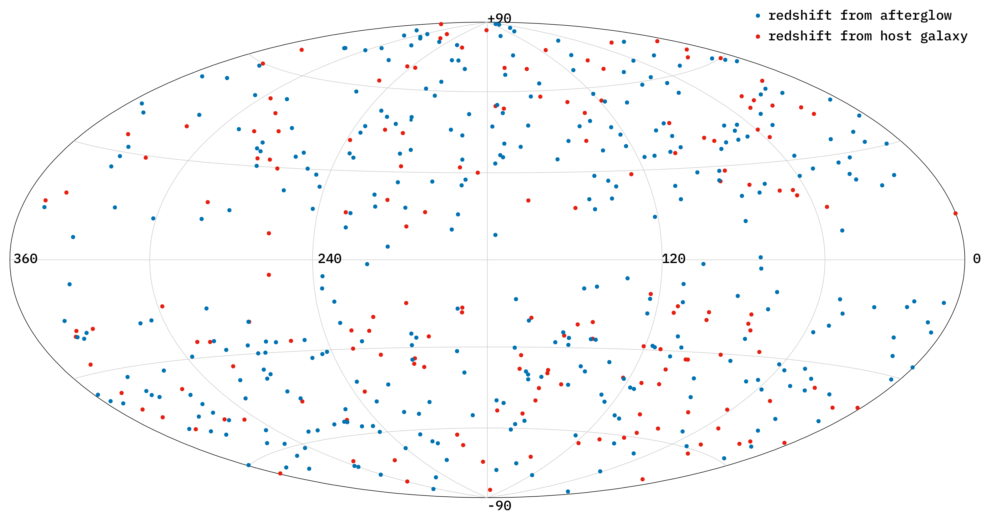
7] with new observations, till 4 June 2021. Greiner’s table and the relevant Gamma-ray Coordination Network messages were also used to enhance the data. This process resulted in a total of 522 GRBs with precise position and spectroscopic redshift. The redshift’s optical observation type according to afterglow or host galaxy detection is registered as well. The galactic distribution of these 522 GRBs is shown on
Figure 1, according to the redshift origin (afterglow or host galaxy measurement).
This GRB positional set is the largest available, worthwhile for a large-scale homogeneity and isotropy check. One should remark that after 2006, the well-localized GRBs rate was ≈120/year, but later, it decreased almost with an exponential decay: every year, the results were only ≈90% of the previous year’s redshift observations [
7]. This trend was halted only in recent years by a few optical campaigns with really committed observers. However, the current rate of the new redshift observations is low, which makes the chance of the substantial statistical improvements low in the near future.
We calculated and used the comoving distances based on the observed spectroscopic redshifts. Following the results of Planck Collaboration et al. [
8], we took
, and
km/s for the calculations. As we are concentrating on the large-scale distribution of the GRBs, we omitted the nearest 500 Mpc observations, this length being ≈2× the BAO distance. In
Figure 2, the comoving distance distribution is shown for our GRBs.
It should be remarked that the observational errors in the redshift measurements are small, usually in the range. We used the errors when present in the observation record and estimated with the last digit of the z value for the rest. The radial errors follow an approximately log-normal distribution, with 0.31, 1.46, and 3.16 Mpc for the first quartile, median, and third quartile. The distribution does not depend on the afterglow/hosts distinction. For the full-3D positional errors, the reported positional uncertainties were also considered, producing slightly larger 0.35, 1.65, and 3.60 Mpc values for the first quartile, median, and third quartile. These errors do not affect our distance calculations practically.
3. Large-Scale Anomalies Observed Earlier
3.1. Compton Gamma-Ray Observatory BATSE’s Observations
The first indirect observational proof for the GRBs’ cosmological origin was reported by Meegan et al. [
9]: after the first 2 years of BATSE observations, the observed GRBs showed an almost isotropic distribution without any concentration around the Galactic plane.
Briggs [
10] proposed the Rayleigh–Watson and the Bingham statistics to test the point source distribution’s dipole and quadrupole anisotropies. Briggs et al. [
11] used dipole and quadrupole statistics for the BATSE GRBs’ sky distribution and found no deviation from the large-scale isotropy at the
level for the dipole and the
level for the quadrupole term. These results strengthened the cosmological origin model of the sources.
Using angular positional measurements only from the BATSE experiment, Balázs et al. [
12] found that the sky distributions of short and long GRBs are different. They compared the quadrupole term, which is non-zero, with a probability of 99.97%.
The very short (with
s) GRBs’ sky distribution have been shown to be anisotropic by Cline et al. [
13] and Cline [
14] with a
level (the non-uniformity in the sky exposure was neglected).
Considering the non-uniform BATSE sky exposure, Chen and Hakkila [
15] analyzed the sky exposure regarding the Two-Point Angular Correlation Function and found that the sky exposure effects are small. However, the non-uniform sky exposure complicated all detailed statistics, so it should have been taken care of.
A BATSE-modified count-in-cell method, which compensates for the well-known Sky Exposure Function, was applied on the GRB data: it was found that the distribution of the intermediate class (where 2 s
s) is not isotropic on the 99.3% confidence level [
16]. Mészáros et al. [
17] used the method of spherical harmonics for the investigation of the angular distribution of the same intermediate group and found that it shows an intrinsic anisotropy at the 97% significance level. Litvin et al. [
18] confirmed the anisotropy for the short bursts with a higher 99.99% significance level, while for the intermediate class, anisotropy only, a lower 99.89% significance level was obtained.
On the 2–5
angular scale, Magliocchetti et al. [
19] found significant correlation among the short GRBs at a level of ∼
. Tanvir et al. [
20] confirmed a correlation between the short GRBs’ position and the positions of galaxies in the local Universe at a 99.9% level.
Using the full BATSE data, it has also been shown using extensive combined statistics (using Voronoi tessellation, minimal spanning tree, and multifractal spectrum) that the short GRBs deviate significantly from the full randomness at a 99.90–99.98% level, while the intermediate group showed a weaker, but still significant deviation from the full isotropy at a 98.51% level [
21]. Extensive Monte Carlo simulations were applied to compensate for the BATSE’s sky exposure function.
3.2. The Hercules-Corona Borealis Great Wall
The largest observed structure in the Universe so far was identified as a large GRB cluster at redshift
in the general direction of the constellations of Hercules and Corona Borealis [
22].
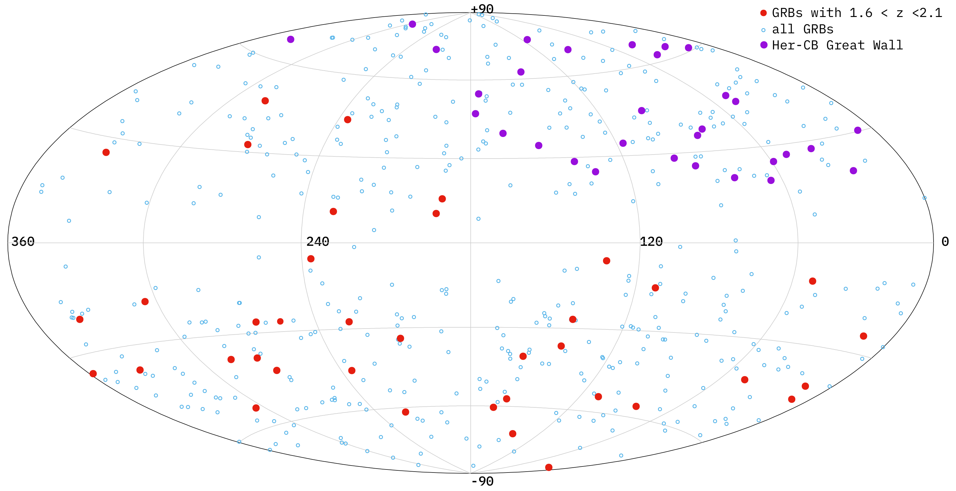
The size of the Hercules-Corona Borealis Great Wall is estimated to be about 2–3 Gpc across (
Figure 3); the uncertainties are mainly due to the sparse sampling. This clustering’s scale is quite large: if it reflects the underlying distribution of matter, the cluster is big enough to question standard assumptions about Universal homogeneity and isotropy.
Horvath et al. [
22] used 283 GRB with redshifts to investigate the spatial distribution of GRBs. They assumed that the sky exposure is independent of
z; therefore, they subdivided the GRB sample by redshift. Angular tests were applied on nine groups based on redshift/distance, using
k-th nearest neighbor analysis and the bootstrap point radius method on their dataset. Nearest neighbor tests identified pairing consistent with the previously found large, loose GRB cluster in the redshift range
.
The observed angular excess cannot be entirely attributed to the known selection biases, making its existence due to chance unlikely. The significance of this cluster can be measured using the bootstrap point–radius method where one selects random locations on the celestial sphere and finds how many of the points lie within a circle of a predefined angular radius. The analysis can be performed with the clustered 44 GRBs and also with 44 random samples from the full observed dataset [
23]. The probability that this clustering is random is
. The direction of the cluster is
,
.
The initial discovery was supported by subsequent observations [
7,
23], although the exact nature of the structure is still unknown partially due to the sparse data. Horvath et al. [
7] divided the data into six radial GRB groups and found the
group to be the most anisotropic. They suggested incorporating the sky exposure for a more detailed spatial analysis—this is what we used for the Spatial Two-Point Correlation Function calculations in
Section 4. In
Figure 3, the relevant
range is shown in our current GRB data.
3.3. The Giant GRB Ring
Balázs et al. [
24], motivated by the Hercules-Corona Borealis Great Wall, analyzed the
k-th nearest neighbor in the sample further. Instead of the slices in the redshift range, the
k-th Next Neighbor Statistics was used to determine the spatial density of the GRBs. Multiple
k values were used to calculate the mean and variance of the local density at every GRB location and, it was found that in the cases of
, the grouping of nine objects deviates significantly from the random case.
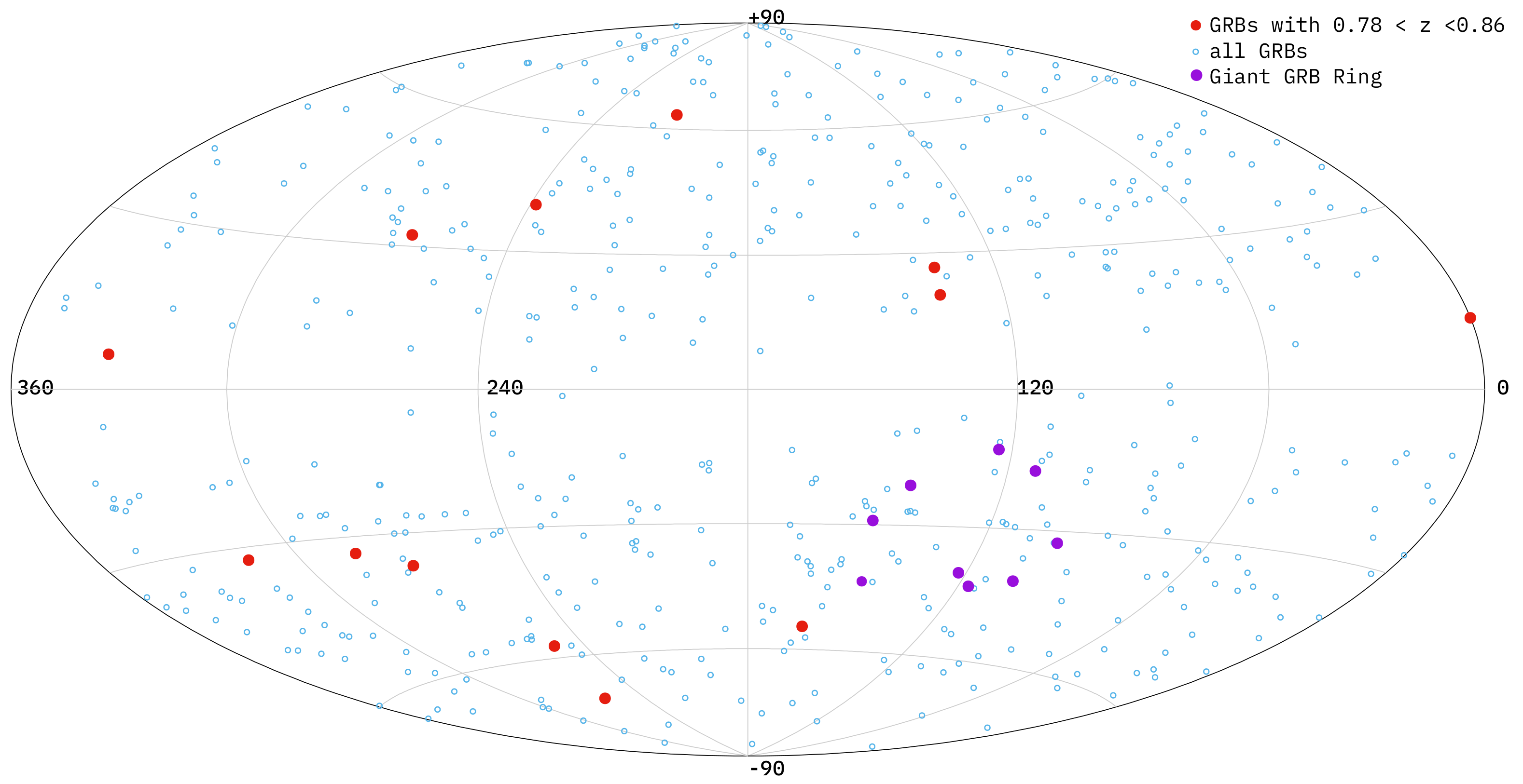
During the analysis, a large regular formation of GRBs was found: the Giant GRB Ring is displayed by nine GRBs, with an angular major/minor diameter of
, at a comoving distance of ≈2.77 Gpc in the
redshift range, with a probability of
of being the result of a random fluctuation only [
25]. The size is ≈1.7 Gpc, a bit smaller than the Hercules-Corona Borealis Great Wall, but larger than the large quasar group (
Mpc, [
26]). In
Figure 4, the Giant GRB Ring’s
redshift range is shown using current GRB data.
Regarding the Giant GRB Ring, Balázs et al. [
25] used different statistical methods to analyze the statistical properties of the spatial point process displayed by GRBs of known redshift. They used kernel-smoothing for the the joint probability density estimation, while the independence of the angular and radial variables of the GRBs was supposed. With 1502 random datasets, they found only three ring-like patterns having similar parameters as the original one appearing in the Ring; thus, the Giant GRB Ring’s existence is a low-probability random event. They also warned that the large-scale GRB distribution does not necessarily reflect the large-scale distribution of the matter.
3.4. Large-Scale Distribution and Physical Properties of GRBs
There are at least two different types of GRB central engines: the merging of compact objects, such as neutron stars and/or black holes, will probably produce short GRBs, confirmed by, e.g., the kilonova observation of Tanvir et al. [
27] and the GRB170817A event [
28]. Collapsing massive stellar objects are connected to the long GRBs [
29]. There are some indications for the existence of a third, intermediate group [
30,
31,
32,
33,
34], and using different observed parameters and spectral models, the classification could be extended [
35].
The early CGRO BATSE observation anisotropy investigations [
12,
13,
16,
17,
18,
19,
21] have shown that the major GRB groups, especially the short and the long one, show different sky distribution. They are important from the sky exposure point of view: if events with different observed length have the same observation probability, the anisotropy effects should be real. Therefore, any correlation between the physical parameters and the sky distribution is important.
Tarnopolski [
36] used the sky distribution of 1669 Fermi/GBM GRBs for the binomial test, nearest neighbor, fractal dimension, dipole and quadrupole analysis, and the two-point angular correlation tests. The results showed that short GRBs are distributed anisotropically in the sky with a probability of 99.98%, while the long GRBs showed no anisotropy. In Bagoly et al. [
37], 361 GRBs with position and redshift were analyzed, and the large-scale homogeneous and isotropic distribution was checked using nearest neighbor tests and the two-point correlation function. Shirokov et al. [
38] analyzed the spatial distribution of 384 Swift GRBs with known redshifts using conditional density and pairwise distance methods. They estimated a fractal dimensionality of D = 2.55 on scales of 2–6 Gpc.
Andrade et al. [
39] tested the sky distribution isotropy of the FERMI-GBM catalogue’s 2626 GRBs. The large positional uncertainties in the positions prevented the applied two-point angular correlation function from detecting any statistical anisotropy, both for the long and short GRBs.
Wang et al. [
40] analyzed some intrinsic properties of 6289 GRBs using prompt and afterglow parameters, searching for correlations between the parameters and the classification of the GRBs.
Cao et al. [
41] used the Platinum GRB data compilation to create standardizable events in the Dainotti correlation space. The obtained GRB cosmological parameter limits are consistent with the baryon acoustic oscillation (BAO) and Hubble parameter [H(z)] data. In Cao et al. [
42], Dainotti-correlated gamma-ray burst were standardized and used to constrain cosmological model parameters. The results provide limits on the non-relativistic matter density, slightly favoring non-zero spatial curvature.
Řípa and Shafieloo [
43] used the Fermi/GBM GRB catalog to test the correlation between GRBs’ durations, fluences, peak fluxes measured in different energy, and the sky positions of the GRBs. Řípa and Shafieloo [
44] expanded the data with the BATSE and Swift BAT GRBs. The tests showed no correlation between the sky positions and the physical properties of the GRBs.
Recently, Horvath et al. [
45] investigated the connection between the GRBs’ durations and redshifts/radial distances and also found no correlation between them.
These results are consistent with a view that the GRBs physical parameters are independent of their position in the Universe.
3.5. Quasar Positions and Polarizations
Although we do not know precisely how the GRBs and the visible matter distributions are related, the quasars’ distribution in the Universe could give some hints about the baryonic matter distribution. The quasars’ high luminosities and early emission make them appropriate for large-scale surveys besides the GRBs.
Jain et al. [
46] analyzed the polarization of quasar emission with parallel transport techniques. The statistical results support the existence of the large-scale alignment effect in the
quasar optical polarization observations. Pelgrims and Hutsemékers [
47] found significant large-scale alignments of polarization vectors among quasars using 2D and 3D statistical methods. Using 71 quasars at redshifts 1.0 < z < 1.8, Friday et al. [
48] reported correlated orientations of their optical and radio polarization on Gpc scales.
Clowes et al. [
26] analyzed the spatial distribution of quasars, claiming the existence of a structure with a size above 1 Gpc. Marcha and Browne [
49] used two-point correlation functions to analyze the clustering of Fermi-selected BL Lac objects and Fermi-selected flat spectrum radio quasars. Separating the BL Lac-like objects with machine learning classifications based only on gamma-ray information, they found evidence for large-scale clustering amongst them. As an explanation for the clustering, they proposed that there are indeed large volumes of space in which AGN axes are aligned.
Lopez et al. [
50] analyzed the distribution of the intervening MgII absorbers in the spectra of background quasars and found a “Giant Arc on the Sky” at
. Its size is ∼1 Gpc and appears to be almost symmetrical on the sky.
3.6. Theoretical Remarks about the Anisotropies
The existence of the above-mentioned anomalies raises the question about their origin. Without full analysis, we list some theories. See [
51] for an overview of the standard
CDM model’s tensions problem and other current cosmological challenges.
One source could be some real cosmic anisotropy, e.g., Ciarcelluti [
52] studied the anisotropic cosmic expansions with electrodynamics, predicting the appearance or variation of the polarization of electromagnetic radiation regarding these regions. Migkas et al. [
53] analyzed 570 clusters with X-ray, microwave, and infrared observations to create scaling relations. Using all available distance information, they detected an apparent 9% dipole-like spatial variation in the local
at
on the sky. The result could also be attributed to a 900 km/s bulk flow. Any variation in the
will create different radial scales and would produce an anisotropy signal.
There could be several astrophysical reasons for the clustering of GRBs [
7]. The low metallicity massive stars are thought to be long GRB progenitors as they generally appear in faint, blue, low-mass star-forming galaxies [
54,
55] and in the bright regions of the host galaxy [
56,
57,
58]. Short GRBs are not expected to trace star-forming activity due to the long inspiralling time of the binary. This notwithstanding, Palmerio et al. [
55] claims that long GRBs are not good tracers of star formation, based on the result of the Swift GRB Host Galaxy Legacy Survey, covering
. Bagoly et al. [
59] studied the distribution of the starburst galaxies from the Millennium XXL Simulation [
60]. With Markov Chain Monte Carlo simulations, the connection between the large-scale structures and the starburst galaxies’ groups distribution were checked at the Giant GRB Ring’s
distance. Using the same simulation, Balázs et al. [
24] demonstrated that the spatial distribution of galaxies with a normal vs. high star-formation rate is probably different. Hence, speculations about some fluctuation or a wave in star formation rate is too simple to describe the full view.
4. The Sky Exposure Function
4.1. Correlation between the Redshift and Sky Position
We know that the observational probability of a GRB differ on the sky, due to the various effects (geometrical, satellite operation, optical follow-ups). As we saw in
Section 3.4, no known correlations have been found between the GRBs’ direction and their physical properties.
For the reconstruction of the full three-dimensional GRB distribution, the main question is whether the sky distribution is independent of the redshift (comoving radial distance) or not. We tested this correlation in the following way: around each GRB, the radial distance distribution of the neighboring GRBs within an
-sized spherical cap were determined. The Mann-Whitney U-test’s Z score was determined between the full and the local dataset using the full radial distribution (i.e.,
Figure 2). As the full dataset contains the local data, as well, we performed Monte Carlo randomization and determined the Z score distribution for a total random local dataset. The whole process was repeated for the
range for 1000 random datasets each. The result are shown in
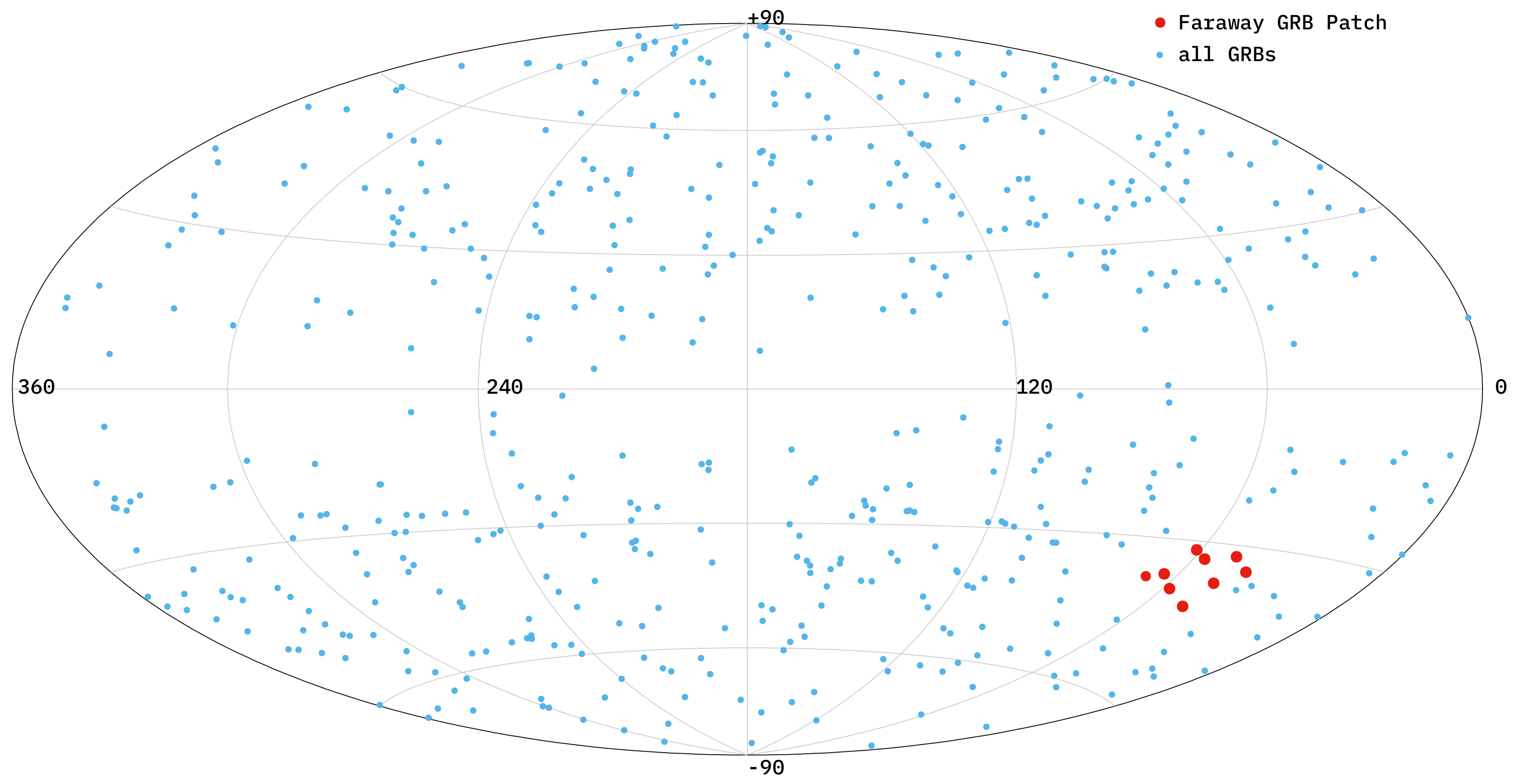
Figure 5: all the 99%, 99.5% and 99.9% values of the Monte Carlo simulations, as well as the smallest Z score from the real data (the second smallest values are above the 99% curve of the Monte Carlo simulations).
This method selects an interesting region with a spherical cap size of 12–14
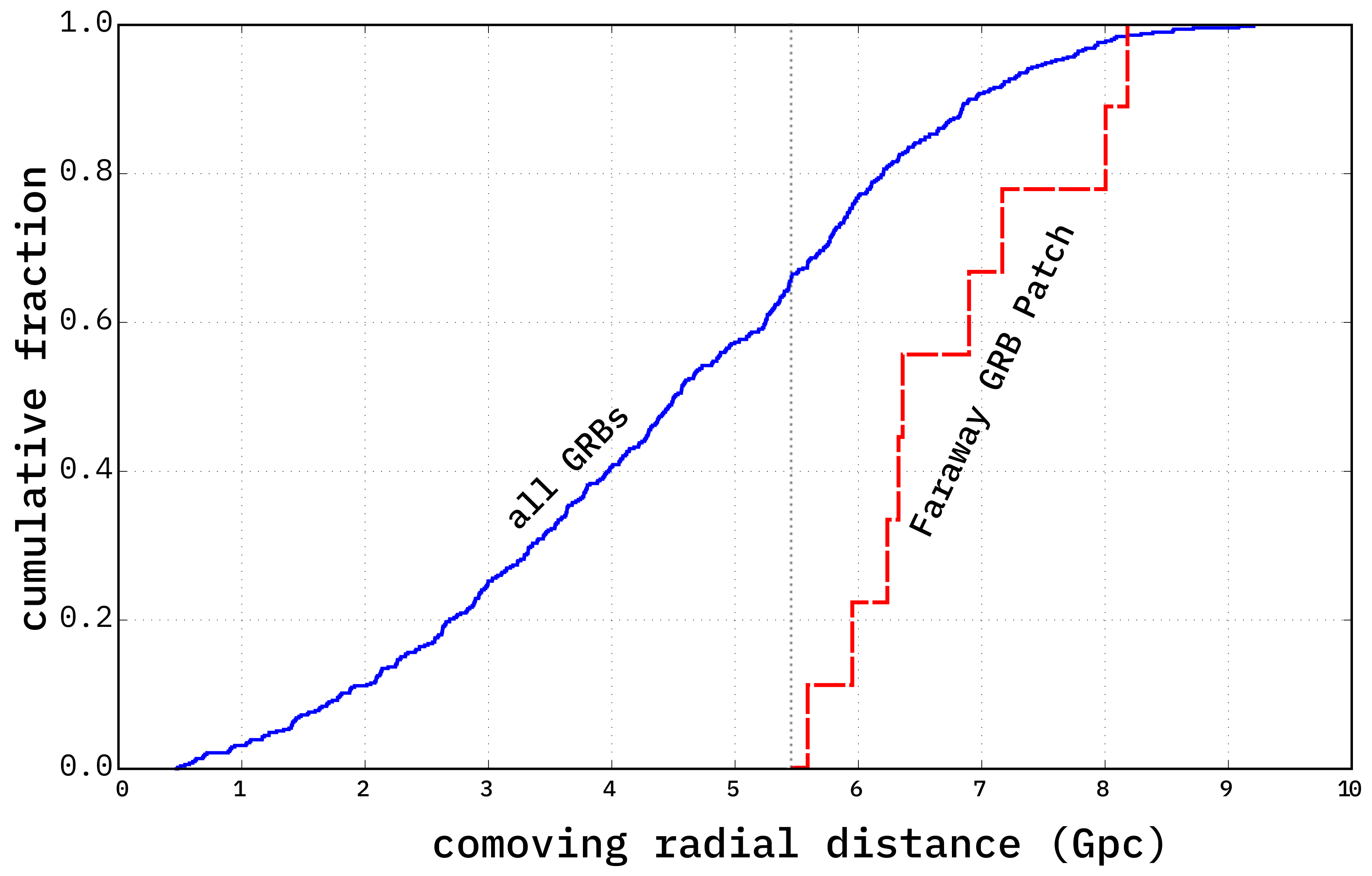
, with a corresponding random probability of ≈1%. This signal is from one region, the Faraway GRB Patch (
Figure 6), where nine distant GRBs are concentrated (
Figure 2). All redshifts are from afterglow observations for the Faraway GRB Patch.
The ≈1% random probability of the Faraway GRB Patch makes it interesting; however, it is large enough not to be considered a real strong signal. Another factor is that we repeated the test many times, and there was a correlation between the tests, as the same overlapping data were used. For the spherical cap, there are ≈60 separate regions on the sky, i.e., this should be the minimum value considered for the correction factor.
Our results show that the sky and the radial component of the GRB distribution could be factorized and both can be determined independently.
4.2. Optical Observational Factors
The detection probability of the redshift-determined GRBs on the sky is a multi-parameter event. The detection probability depends on the various trigger and detection conditions of the space instruments, the optical follow-up procedure, etc.
The simplest models for the sky exposure could be created, e.g., using the pointing logs of the satellite. From a theoretical point of view, one can imagine that it is possible to integrate the satellite’s FOV timeline (e.g., Swift and/or Fermi GBM pointings) and simulate all the (known) triggering effects, including the background changes. Beside this, one would still need to combine it with a reliable model for selection effects including the impact of galactic extinction and the various optical observational effects and constraints (e.g., timing, sky visibility, telescope/instrument availability, observer interest, etc.). Here, we investigate the available dataset and show that this is practically not feasible as it cannot be done with the required precision due to both technical and human factors.
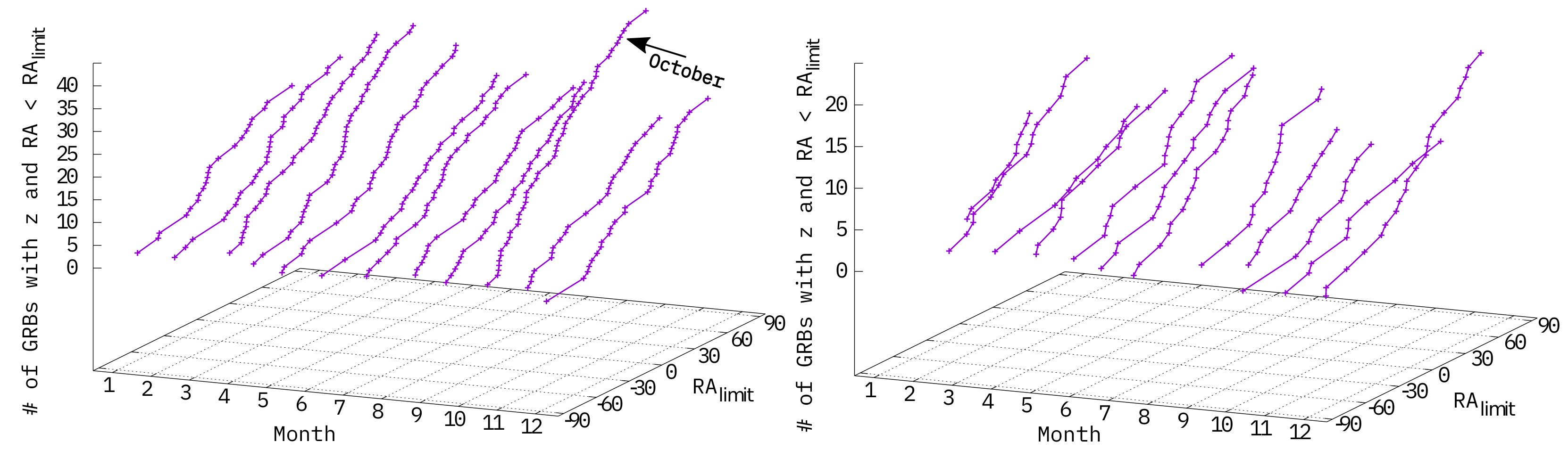
In
Figure 7, we plot the
N(>
RA) cumulative number of GRBs as a function of the
right ascension, for every month. All 522 GRBs from the current data were used. Here, we split the data according to the observations: redshift determined from afterglow means that prompt (or almost prompt) observations was performed—there are 354 such GRBs in our sample. Host galaxy observations could be done later; therefore, it is possible that the observational limits and strategies are different. We have 168 redshifts from host galaxy measurements. Campaigns and dedicated projects were (and hopefully will be) organized to measure the redshift of the known host galaxies: sometimes, this is done years after the GRB. The dichotomy between the afterglow and host galaxy determined redshift grouping is boosted further by the fact that host-based observations are rare above
, i.e., their average redshift is lower.
One would expect a smoothly varying distribution, considering the various influences of the telescope geographic position and availability, weather, projects, etc. The afterglow and host galaxy measurements follow approximately the same pattern with quite similar yearly modulation, except the afterglow’s October distribution. The extra ≈ 10–15 observations were created probably by other factors, such as a dedicated rapid response afterglow fall campaign.
4.3. Kernel-Based Estimation of the Sky Exposure Function
As the synthetic way is not quite viable, we can use only the observational data themselves to derive the detection probability on the sky. This is not a paradox: assuming the sky distribution independent of the redshift (see
Section 4.1), the dataset-averaged sky detection probability can be approximated and used as a reference.
In Bagoly et al. [
61], the optimal empirical Sky Exposure Function was reconstructed with different techniques. The Swift’s exposure map was used as a model for the GRB-like angular distribution. The efficiency of the fixed and the adaptive width Gaussian kernel, the Delaunay Tessellation Field Estimator, and the Voronoi Diagram Field Estimator methods were compared on a random field, similar to the Swift’s exposure map. It was determined that the fixed-width Gaussian kernel is the optimal among the methods for approximating the exposure map and for determining the optimal width.
In Li and Lin [
62], Bagoly et al. [
37], as well as Ukwatta et al. [
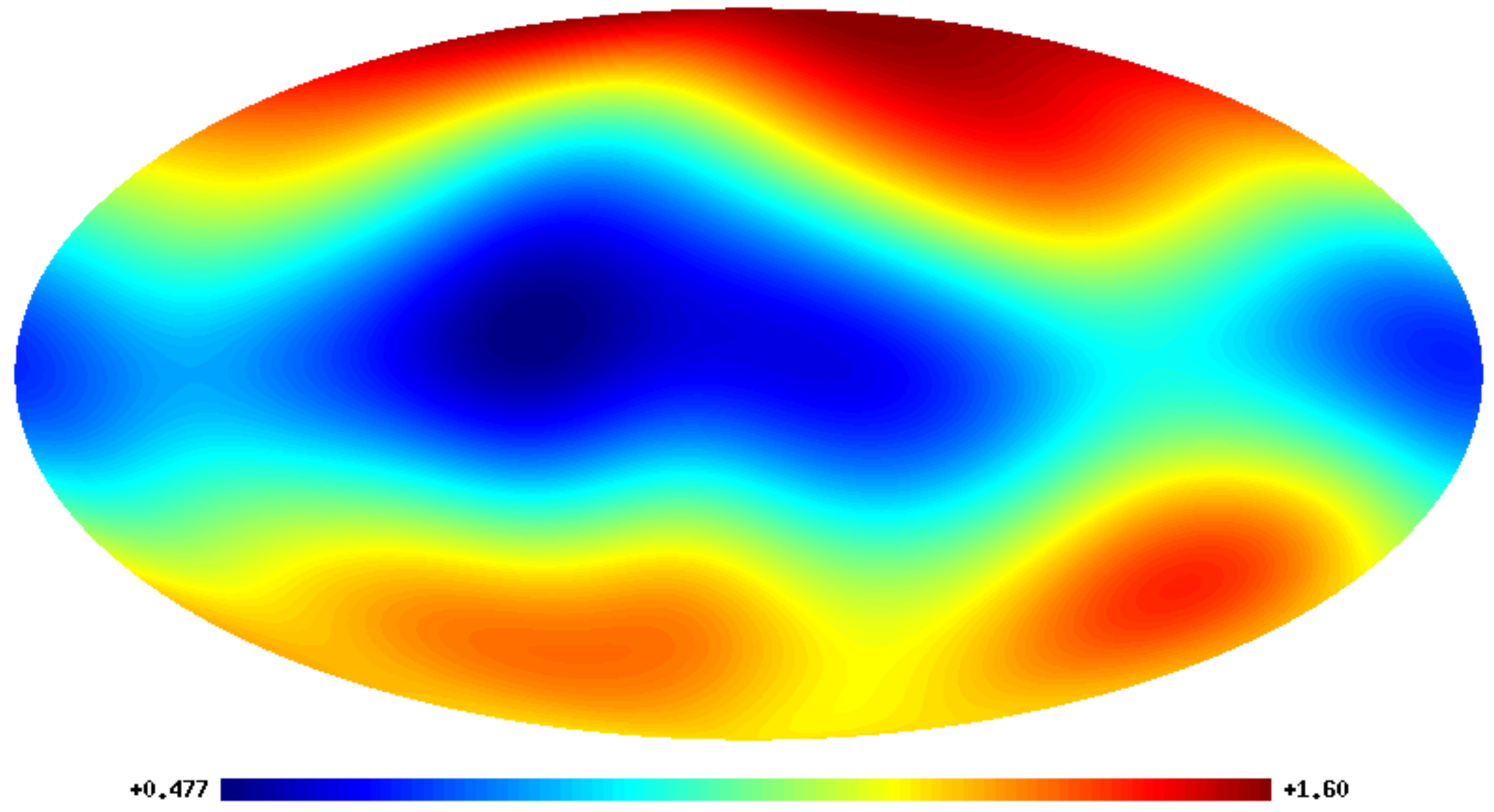
63], kernel-based methods were applied in the reconstruction of the GRBs’ empirical Sky Exposure Function. We applied Gaussian kernel-smoothing on the current GRB data to obtain the empirical Sky Exposure Function. In
Figure 8, one can observe the optimal kernel-smoothed Sky Exposure Function. There is a factor of ≳3 between the minimum and maximum, and the galactic disk is visible. The optimal kernel sizes for the typical few hundreds GRBs are in the 20–40
range [
61], clearly bigger than the width of the galactic optical extinction range (cf.
Figure 1). Thus, kernels will produce a smoother sky exposure than the real one, resulting in a lower statistical power for structures’ detection near and below the kernel size.
5. The Spatial Two-Point Correlation Function
Using the empirical Sky Exposure Function of
Figure 8 and the radial distribution (cf.
Figure 2) together, we determined the general Spatial Two-point Correlation Function, which is widely used measure to quantify the large-scale structure. We used the Landy–Szalay method [
64] as the optimal tool for a known partial vignetting and reduced observational probabilities. For the
Spatial Two-Point Correlation Function, one should generate random points according to the spatial detection probability, e.g., here, using the radial distribution and sky exposure. The
,
, and
correlations were calculated between the data–data, data–random, and random–random points. The
Spatial Two-Point Correlation Function will be given by
.
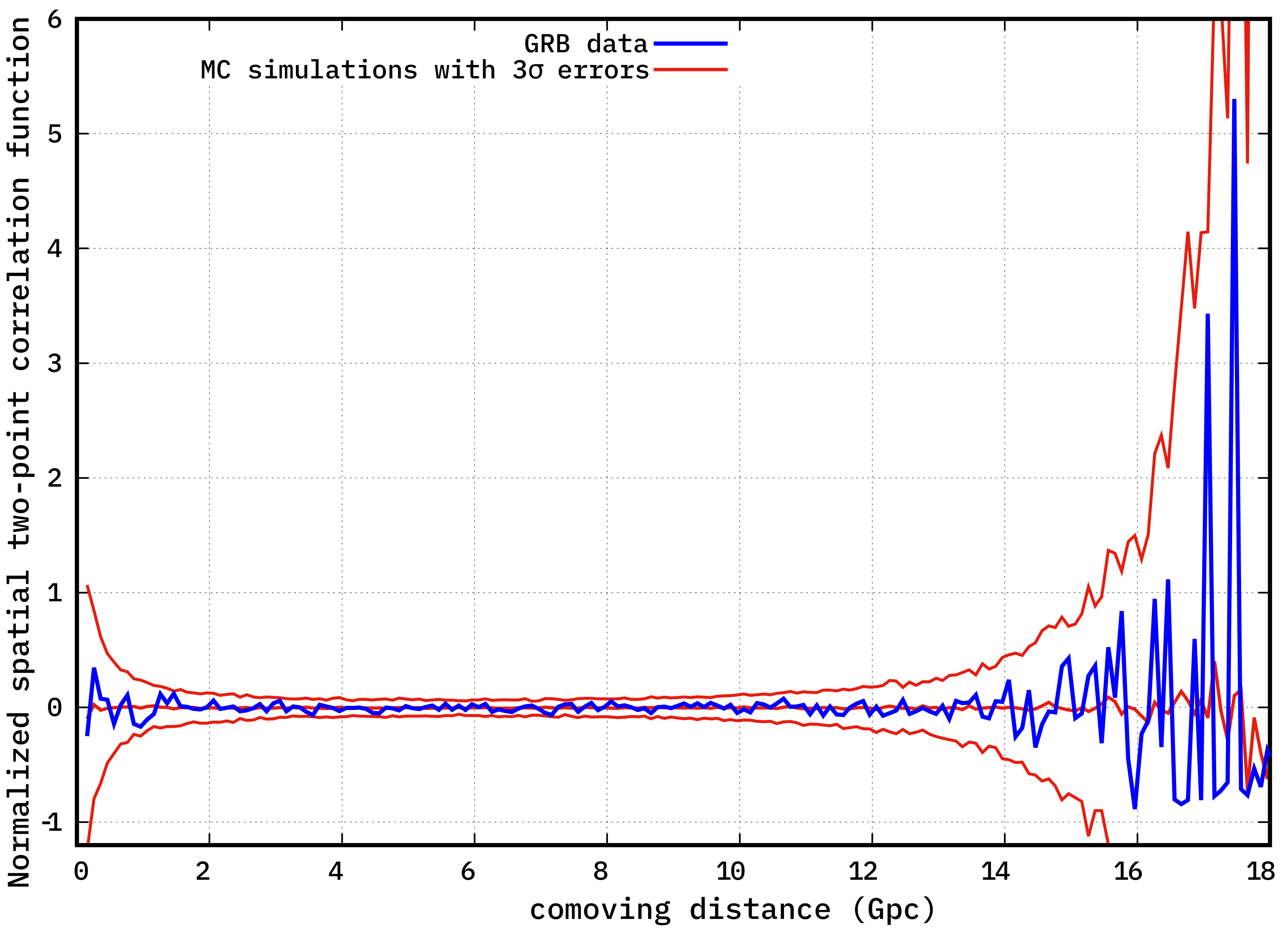
We used 10,000 random points for the calculations and also used 100 synthetic dataset following the same distribution as the data to create Monte Carlo simulations. The from the random datasets were used to determine the Poissonian errors in the calculations.
In
Figure 9, the
of the full dataset are shown, with the mean and
errors. The 100 synthetic datasets’ mean should be 0, and the
error lines mark the noise. All GRB
values are within the errors, and no correlation structure is observable.
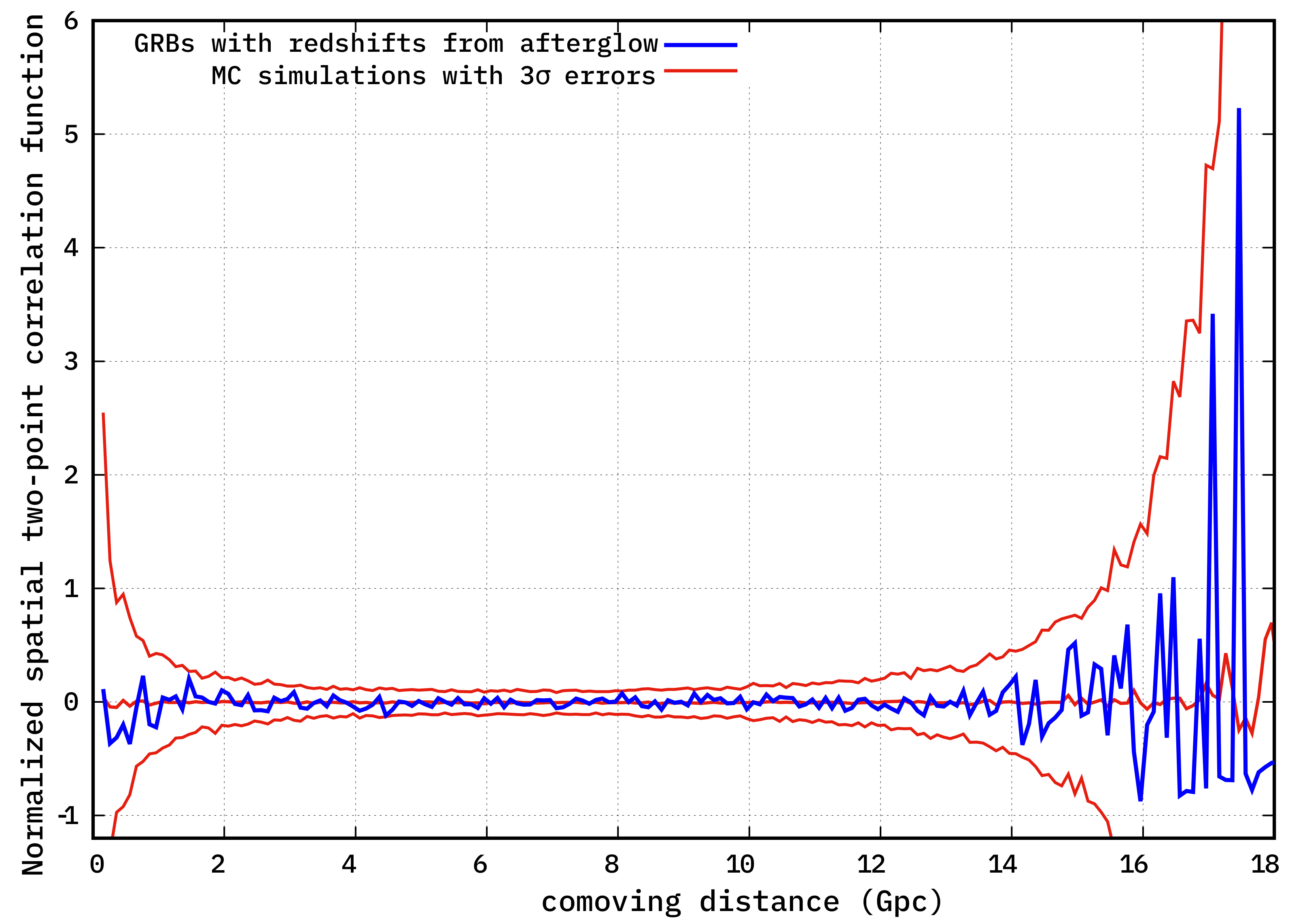
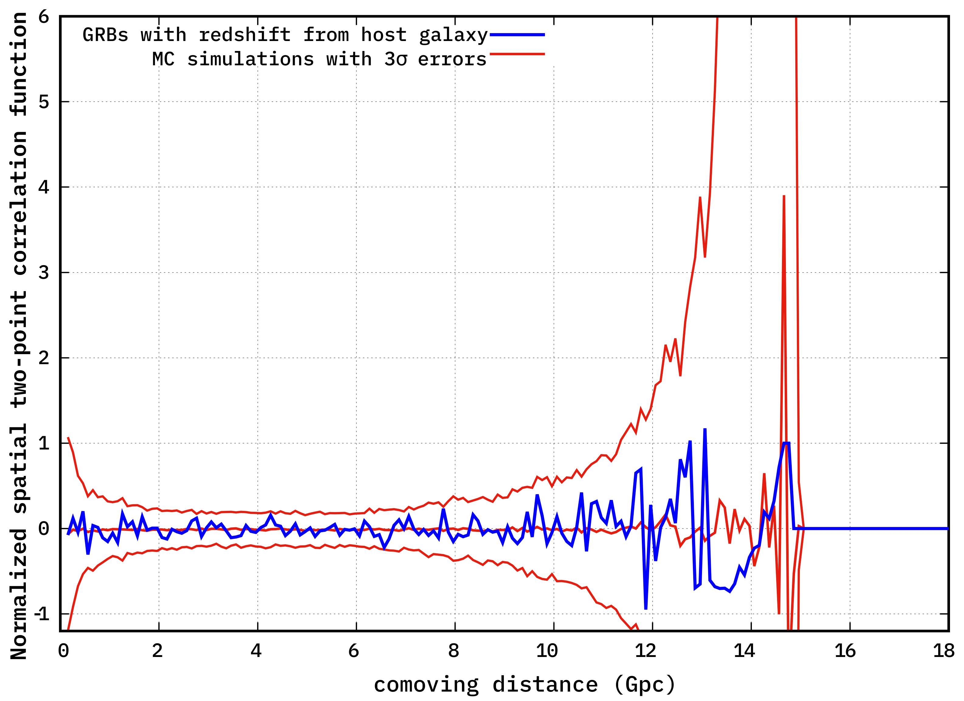
We repeated the same calculations for
using only the afterglow or host galaxy distances. In
Figure 10 and
Figure 11, the corresponding
functions are displayed, with the accompanying errors. In both cases, the GRB
values are within the
errors.
6. Discussion
Kernels will produce a smoother Sky Exposure Function than the real one, smoothing out the distribution and resulting in a lower statistical power for structures’ detection near and below the kernel size. This is possibly why the signals of the Hercules-Corona Borealis Great Wall and/or the Giant GRB Ring are below the lines: they are buried in the noise. It is not surprising that the spatial two-point correlation is not the optimal tool for such huge scales: besides the low-count Poisson noise, the smoothed Sky Exposure Function will reduce the sensitivity of the function to large structures, i.e., structures will be smoothed out on the sky and the statistics will give lower significance. Kernel-generated sky exposure and the related random catalogs will contain some part of the smoothed structures, making the signal smaller in the Landy–Szalay method.
These effects will distort the distribution quite differently at different comoving distances because of the angular distance scale’s saturation, e.g., for , the comoving distance is ≈2.7 Gpc and the transverse scale is ≈530 Mpc, while the comoving distance is ≈4.5 Gpc with a transverse scale of ≈600 Mpc. Hence, the kernel-smoothing is suboptimal as it introduces distortions similar to the redshift space distortions: here, transversal smoothing is experienced, while in the classic redshift measurements, the peculiar velocity components along the line of sight will smear the signal.
One should consider that in Bagoly et al. [
61], the 2-year Swift exposure map was used as a benchmark. It is a relatively smooth function due to the large (>90
) BAT aperture, and the best method was selected using this objective function. In
Figure 1, one can see that the galactic extinction’s effect is acting on a much smaller scale; hence, the best kernel method will definitely oversmooth that region. The low density of the events will further augment the problem.
Clearly, better algorithms should be developed for more precise calculations, such as nearest neighbor analysis-based [
36] methods and similar tools, which incorporate the transverse distortion effect mentioned earlier.
We should remark that Bagoly et al. [
37] used the Spatial Two-Point Correlation Function to identify the interesting GRB 020819B and GRB 050803 pair. In their data, both GRBs had a spectroscopic redshift, and they caused a strong peak in Spatial Two-Point Correlation Function around 56 Mpc, with a probability of 0.00996 being a random fluctuation. Quite interestingly, both GRBs’ redshift values were questioned later in the literature, more than a decade later after the events. The Optically Unbiased GRB Host (TOUGH) survey [
65] measured
photometric redshift for the host galaxy of GRB 050803, unlike the previous preliminary
value, and thus, we omitted this GRB from the dataset. Perley et al. [
66] analyzed the purported spiral host galaxy of GRB 020819B at
and used VLT MUSE and X-shooter observations to demonstrate that it is an unrelated foreground galaxy. They identified a possible radio afterglow with a star-forming galaxy at
, which is consistent with the observations. Hence, as both previous estimated distances are probably wrong and the new values are differ significantly, the peak observed in Bagoly et al. [
37] obviously should not appear in these results.
7. Summary
We overviewed the previous statistical analyses and results regarding the GRBs’ sky and spatial distribution, and in
Section 4, we determined some of the various factors influencing the optical observations.
We analyzed the possible correlation between the GRB redshift and sky position. The GRB distance distribution in a spherical cap was compared with the full distribution using the Mann-Whitney U test’s Z score. There was only one region, called the Faraway GRB Patch, where nine distant GRBs showed a deviation from the randomness with an ≈1% probability. This show that the sky and the radial component of the GRB distribution could be factorized and both can be determined independently.
The GRBs’ cumulative monthly functions show an extra component in the afterglow-determined redshifts’ October distribution. It was probably originated from some dedicated rapid response fall campaign and shows that it is not possible to create the Sky Exposure Function even from the perfect observational logs.
We used the Gaussian kernel to obtain the estimation of the Sky Exposure Function for our 522 GRB. This distribution was used with the radial distribution for the Spatial Two-Point Correlation Function
. Monte Carlo simulations were used to determine the Poissonian errors, while the redshift origin (afterglow or host galaxy) factor was applied to split the data. In
Figure 9,
Figure 10 and
Figure 11, one can see that the current
estimations are consistent with zero for the full and the afterglow/host galaxy datasets.
Author Contributions
Conceptualization, Z.B., L.G.B., I.H., L.V.T. and I.I.R.; data curation, Z.B. and I.I.R.; formal analysis, Z.B. and L.V.T.; investigation, Z.B., I.H. and L.G.B.; methodology, Z.B., I.H. and L.V.T.; project administration, Z.B.; resources, Z.B., I.H. and I.I.R.; software, Z.B., I.H. and I.I.R.; supervision, L.G.B., Z.B., I.H., L.V.T. and I.I.R.; validation, Z.B., L.G.B., I.H., L.V.T. and I.I.R.; visualization, Z.B. and L.V.T.; writing—original draft, Z.B., L.G.B., L.V.T., I.H. and I.I.R.; writing—review and editing, Z.B., L.G.B., L.V.T., I.H. and I.I.R. All authors have read and agreed to the published version of the manuscript.
Funding
Hungarian TKP2021-NVA-16 and OTKA K134257.
Institutional Review Board Statement
Not applicable.
Informed Consent Statement
Not applicable.
Data Availability Statement
Not applicable.
Acknowledgments
The authors would like to thank Jakub Ripa, Mariusz Tarnopolski, Sándor Pintér, and late Attila Mészáros for numerous discussions on GRBs. We are indebted to Jakub Ripa and Mariusz Tarnopolski for initiating the writing of this paper. The authors thank the Hungarian TKP2021-NVA-16 and OTKA K134257 program for their support.
Conflicts of Interest
The authors declare no conflict of interest.
References
- Wang, F.Y.; Dai, Z.G.; Liang, E.W. Gamma-ray burst cosmology. New Astron. Rev. 2015, 67, 1–17. [Google Scholar] [CrossRef]
- Wang, J.S.; Wang, F.Y.; Cheng, K.S.; Dai, Z.G. Measuring dark energy with the Eiso- Ep correlation of gamma-ray bursts using model-independent methods. Astron. Astrophys. 2016, 585, A68. [Google Scholar] [CrossRef]
- Amati, L.; D’Agostino, R.; Luongo, O.; Muccino, M.; Tantalo, M. Addressing the circularity problem in the Ep- Eiso correlation of gamma-ray bursts. Mon. Not. R. Astron. Soc. 2019, 486, L46–L51. [Google Scholar] [CrossRef]
- Khadka, N.; Ratra, B. Constraints on cosmological parameters from gamma-ray burst peak photon energy and bolometric fluence measurements and other data. Mon. Not. R. Astron. Soc. 2020, 499, 391–403. [Google Scholar] [CrossRef]
- Demianski, M.; Piedipalumbo, E.; Sawant, D.; Amati, L. Prospects of high redshift constraints on dark energy models with the Ep,i- Eiso correlation in long gamma ray bursts. Mon. Not. R. Astron. Soc. 2021, 506, 903–918. [Google Scholar] [CrossRef]
- Luongo, O.; Muccino, M. A Roadmap to Gamma-Ray Bursts: New Developments and Applications to Cosmology. Galaxies 2021, 9, 77. [Google Scholar] [CrossRef]
- Horvath, I.; Szécsi, D.; Hakkila, J.; Szabó, Á.; Racz, I.I.; Tóth, L.V.; Pinter, S.; Bagoly, Z. The clustering of gamma-ray bursts in the Hercules-Corona Borealis Great Wall: The largest structure in the Universe? Mon. Not. R. Astron. Soc. 2020, 498, 2544–2553. [Google Scholar] [CrossRef]
- Collaboration, P.; Aghanim, N.; Akrami, Y.; Ashdown, M.; Aumont, J.; Baccigalupi, C.; Ballardini, M.; Banday, A.J.; Barreiro, R.B.; Bartolo, N.; et al. Planck 2018 results. VI. Cosmological parameters. Astron. Astrophys. 2020, 641, A6. [Google Scholar] [CrossRef]
- Meegan, C.A.; Fishman, G.J.; Wilson, R.B.; Paciesas, W.S.; Pendleton, G.N.; Horack, J.M.; Brock, M.N.; Kouveliotou, C. Spatial distribution of gamma-ray bursts observed by BATSE. Nature 1992, 355, 143–145. [Google Scholar] [CrossRef]
- Briggs, M.S. Dipole and Quadrupole Tests of the Isotropy of Gamma-Ray Burst Locations. Astrophys. J. 1993, 407, 126. [Google Scholar] [CrossRef]
- Briggs, M.S.; Paciesas, W.S.; Pendleton, G.N.; Meegan, C.A.; Fishman, G.J.; Horack, J.M.; Brock, M.N.; Kouveliotou, C.; Hartmann, D.H.; Hakkila, J. BATSE Observations of the Large-Scale Isotropy of Gamma-Ray Bursts. Astrophys. J. 1996, 459, 40. [Google Scholar] [CrossRef]
- Balázs, L.G.; Mészáros, A.; Horváth, I. Anisotropy of the sky distribution of gamma-ray bursts. Astron. Astrophys. 1998, 339, 1–6. [Google Scholar]
- Cline, D.B.; Matthey, C.; Otwinowski, S. Study of Very Short Gamma-Ray Bursts. Astrophys. J. 1999, 527, 827–834. [Google Scholar] [CrossRef]
- Cline, D.B. Primordial Black Holes and the Asymmetrical Distribution of Short GRB Events. In The Role of Neutrinos, Strings, Gravity, and Variable Cosmological Constant in Elementary Particle Physics; Kursunoglu, B.N., Mintz, S.L., Perlmutter, A., Eds.; Springer: Berlin/Heidelberg, Germany, 2001; p. 157. [Google Scholar]
- Chen, X.; Hakkila, J. The two-point angular correlation function and BATSE sky exposure. In Gamma-Ray Bursts, 4th Hunstville Symposium; Meegan, C.A., Preece, R.D., Koshut, T.M., Eds.; American Institute of Physics Conference Series: College Park, MD, USA, 1998; Volume 428, pp. 149–153. [Google Scholar] [CrossRef]
- Mészáros, A.; Bagoly, Z.; Horváth, I.; Balázs, L.G.; Vavrek, R. A Remarkable Angular Distribution of the Intermediate Subclass of Gamma-Ray Bursts. Astrophys. J. 2000, 539, 98–101. [Google Scholar] [CrossRef]
- Mészáros, A.; Bagoly, Z.; Vavrek, R. On the existence of the intrinsic anisotropies in the angular distributions of gamma-ray bursts. Astron. Astrophys. 2000, 354, 1–6. [Google Scholar]
- Litvin, V.F.; Matveev, S.A.; Mamedov, S.V.; Orlov, V.V. Anisotropy in the Sky Distribution of Short Gamma-Ray Bursts. Astron. Lett. 2001, 27, 416–420. [Google Scholar] [CrossRef]
- Magliocchetti, M.; Ghirlanda, G.; Celotti, A. Evidence for anisotropy in the distribution of short-lived gamma-ray bursts. Mon. Not. R. Astron. Soc. 2003, 343, 255–258. [Google Scholar] [CrossRef][Green Version]
- Tanvir, N.R.; Chapman, R.; Levan, A.J.; Priddey, R.S. An origin in the local Universe for some short γ-ray bursts. Nature 2005, 438, 991–993. [Google Scholar] [CrossRef]
- Vavrek, R.; Balázs, L.G.; Mészáros, A.; Horváth, I.; Bagoly, Z. Testing the randomness in the sky-distribution of gamma-ray bursts. Mon. Not. R. Astron. Soc. 2008, 391, 1741–1748. [Google Scholar] [CrossRef][Green Version]
- Horváth, I.; Hakkila, J.; Bagoly, Z. Possible structure in the GRB sky distribution at redshift two. Astron. Astrophys. 2014, 561L, 12H. [Google Scholar] [CrossRef]
- Horváth, I.; Bagoly, Z.; Hakkila, J.; Tóth, L.V. New data support the existence of the Hercules-Corona Borealis Great Wall. Astron. Astrophys. 2015, 584, A48. [Google Scholar] [CrossRef][Green Version]
- Balázs, L.G.; Bagoly, Z.; Hakkila, J.E.; Horváth, I.; Kóbori, J.; Rácz, I.I.; Tóth, L.V. A giant ring-like structure at 0.78 z 0.86 displayed by GRBs. Mon. Not. R. Astron. Soc. 2015, 452, 2236–2246. [Google Scholar] [CrossRef]
- Balázs, L.G.; Rejto, L.; Tusnády, G. Some statistical remarks on the giant GRB ring. Mon. Not. R. Astron. Soc. 2018, 473, 3169–3179. [Google Scholar] [CrossRef]
- Clowes, R.G.; Harris, K.A.; Raghunathan, S.; Campusano, L.E.; Söchting, I.K.; Graham, M.J. A structure in the early Universe at z ∼ 1.3 that exceeds the homogeneity scale of the R-W concordance cosmology. Mon. Not. R. Astron. Soc. 2013, 429, 2910–2916. [Google Scholar] [CrossRef]
- Tanvir, N.R.; Levan, A.J.; Fruchter, A.S.; Hjorth, J.; Hounsell, R.A.; Wiersema, K.; Tunnicliffe, R.L. A ‘kilonova’ associated with the short-duration γ-ray burst GRB 130603B. Nature 2013, 500, 547. [Google Scholar] [CrossRef]
- Von Kienlin, A.; Veres, P.; Roberts, O.J.; Hamburg, R.; Bissaldi, E.; Briggs, M.S.; Burns, E.; Goldstein, A.; Kocevski, D.; Preece, R.D. Fermi-GBM GRBs with Characteristics Similar to GRB 170817A. Astrophys. J. 2019, 876, 89. [Google Scholar] [CrossRef]
- Woosley, S.E.; Bloom, J.S. The Supernova Gamma-Ray Burst Connection. Annu. Rev. Astron. Astrophys. 2006, 44, 507–556. [Google Scholar] [CrossRef]
- Balastegui, A.; Ruiz-Lapuente, P.; Canal, R. Reclassification of gamma-ray bursts. Mon. Not. R. Astron. Soc. 2001, 328, 283–290. [Google Scholar] [CrossRef]
- Horváth, I.; Mészáros, A.; Balázs, L.G.; Bagoly, Z. Where is the Third Subgroup of Gamma-Ray Bursts? Balt. Astron. 2004, 13, 217–220. [Google Scholar]
- Horváth, I.; Balázs, L.G.; Bagoly, Z.; Ryde, F.; Mészáros, A. A new definition of the intermediate group of gamma-ray bursts. Astron. Astrophys. 2006, 447, 23–30. [Google Scholar] [CrossRef]
- Chattopadhyay, T.; Misra, R.; Chattopadhyay, A.K.; Naskar, M. Statistical Evidence for Three Classes of Gamma-Ray Bursts. Astrophys. J. 2007, 667, 1017–1023. [Google Scholar] [CrossRef]
- Pérez-Ramírez, D.; de Ugarte Postigo, A.; Gorosabel, J.; Aloy, M.A.; Jóhannesson, G.; Guerrero, M.A.; Osborne, J.P.; Page, K.L.; Warwick, R.S.; Horváth, I.; et al. Detection of the high z GRB 080913 and its implications on progenitors and energy extraction mechanisms. Astron. Astrophys. 2010, 510, A105. [Google Scholar] [CrossRef]
- Horváth, I.; Hakkila, J.; Bagoly, Z.; Tóth, L.V.; Rácz, I.I.; Pintér, S.; Tóth, B.G. Multidimensional analysis of Fermi GBM gamma-ray bursts. Astrophys. Space Sci. 2019, 364, 105. [Google Scholar] [CrossRef]
- Tarnopolski, M. Testing the anisotropy in the angular distribution of Fermi/GBM gamma-ray bursts. Mon. Not. R. Astron. Soc. 2017, 472, 4819–4831. [Google Scholar] [CrossRef]
- Bagoly, Z.; Horváth, I.; Hakkila, J.; Tóth, L.V. Anomalies in the GRBs’ distribution. In Galaxies at High Redshift and Their Evolution Over Cosmic Time; Kaviraj, S., Ed.; IAU: Paris, France, 2016; Volume 319, p. 2. [Google Scholar] [CrossRef]
- Shirokov, S.I.; Raikov, A.A.; Baryshev, Y.V. Spatial Distribution of Gamma-Ray Burst Sources. Astrophysics 2017, 60, 484–496. [Google Scholar] [CrossRef][Green Version]
- Andrade, U.; Bengaly, C.A.P.; Alcaniz, J.S.; Capozziello, S. Revisiting the statistical isotropy of GRB sky distribution. Mon. Not. R. Astron. Soc. 2019, 490, 4481–4488. [Google Scholar] [CrossRef]
- Wang, F.; Zou, Y.C.; Liu, F.; Liao, B.; Liu, Y.; Chai, Y.; Xia, L. A Comprehensive Statistical Study of Gamma-Ray Bursts. Astrophys. J. 2020, 893, 77. [Google Scholar] [CrossRef]
- Cao, S.; Dainotti, M.; Ratra, B. Standardizing Platinum Dainotti-correlated gamma-ray bursts, and using them with standardized Amati-correlated gamma-ray bursts to constrain cosmological model parameters. Mon. Not. R. Astron. Soc. 2022, 512, 439–454. [Google Scholar] [CrossRef]
- Cao, S.; Khadka, N.; Ratra, B. Standardizing Dainotti-correlated gamma-ray bursts, and using them with standardized Amati-correlated gamma-ray bursts to constrain cosmological model parameters. Mon. Not. R. Astron. Soc. 2022, 510, 2928–2947. [Google Scholar] [CrossRef]
- Řípa, J.; Shafieloo, A. Testing the Isotropic Universe Using the Gamma-Ray Burst Data of Fermi/GBM. Astrophys. J. 2017, 851, 15. [Google Scholar] [CrossRef]
- Řípa, J.; Shafieloo, A. Update on testing the isotropy of the properties of gamma-ray bursts. Mon. Not. R. Astron. Soc. 2019, 486, 3027–3040. [Google Scholar] [CrossRef]
- Horvath, I.; Racz, I.I.; Bagoly, Z.; Balázs, L.G.; Pinter, S. Does the GRB Duration Depend on Redshift? Universe 2022, 8, 221. [Google Scholar] [CrossRef]
- Jain, P.; Narain, G.; Sarala, S. Large-scale alignment of optical polarizations from distant QSOs using coordinate-invariant statistics. Mon. Not. R. Astron. Soc. 2004, 347, 394–402. [Google Scholar] [CrossRef]
- Pelgrims, V.; Hutsemékers, D. Polarization alignments of quasars from the JVAS/CLASS 8.4-GHz surveys. Mon. Not. R. Astron. Soc. 2015, 450, 4161–4173. [Google Scholar] [CrossRef]
- Friday, T.; Clowes, R.G.; Williger, G.M. Correlated orientations of the axes of large quasar groups on Gpc scales. Mon. Not. R. Astron. Soc. 2022, 511, 4159–4178. [Google Scholar] [CrossRef]
- Marchã, M.J.M.; Browne, I.W.A. Large-scale clustering amongst Fermi blazars; evidence for axis alignments? Mon. Not. R. Astron. Soc. 2021, 507, 1361–1368. [Google Scholar] [CrossRef]
- Lopez, A.M.; Clowes, R.G.; Williger, G.M. A Giant Arc on the Sky. arXiv 2022, arXiv:2201.06875. [Google Scholar]
- Perivolaropoulos, L.; Skara, F. Challenges for ΛCDM: An update. arXiv 2021, arXiv:2105.05208. [Google Scholar]
- Ciarcelluti, P. Electrodynamic Effect of Anisotropic Expansions in the Universe. Mod. Phys. Lett. A 2012, 27, 1250221. [Google Scholar] [CrossRef]
- Migkas, K.; Pacaud, F.; Schellenberger, G.; Erler, J.; Nguyen-Dang, N.T.; Reiprich, T.H.; Ramos-Ceja, M.E.; Lovisari, L. Cosmological implications of the anisotropy of ten galaxy cluster scaling relations. Astron. Astrophys. 2021, 649, A151. [Google Scholar] [CrossRef]
- Le Floc’h, E.; Duc, P.A.; Mirabel, I.F.; Sanders, D.B.; Bosch, G.; Diaz, R.J.; Donzelli, C.J.; Rodrigues, I.; Courvoisier, T.J.L.; Greiner, J.; et al. Are the hosts of gamma-ray bursts sub-luminous and blue galaxies? Astron. Astrophys. 2003, 400, 499–510. [Google Scholar] [CrossRef]
- Palmerio, J.T.; Vergani, S.D.; Salvaterra, R.; Sand ers, R.L.; Japelj, J.; Vidal-García, A.; D’Avanzo, P.; Corre, D.; Perley, D.A.; Shapley, A.E.; et al. Are long gamma-ray bursts biased tracers of star formation? Clues from the host galaxies of the Swift/BAT6 complete sample of bright LGRBs. III. Stellar masses, star formation rates, and metallicities at z > 1. Astron. Astrophys. 2019, 623, A26. [Google Scholar] [CrossRef]
- Fruchter, A.S.; Levan, A.J.; Strolger, L.; Vreeswijk, P.M.; Thorsett, S.E.; Bersier, D.; Burud, I.; Castro Cerón, J.M.; Castro-Tirado, A.J.; Conselice, C.; et al. Long γ-ray bursts and core-collapse supernovae have different environments. Nature 2006, 441, 463–468. [Google Scholar] [CrossRef] [PubMed]
- Blanchard, P.K.; Berger, E.; Fong, W.F. The Offset and Host Light Distributions of Long Gamma-Ray Bursts: A New View From HST Observations of Swift Bursts. Astrophys. J. 2016, 817, 144. [Google Scholar] [CrossRef]
- Lyman, J.D.; Levan, A.J.; Tanvir, N.R.; Fynbo, J.P.U.; McGuire, J.T.W.; Perley, D.A.; Angus, C.R.; Bloom, J.S.; Conselice, C.J.; Fruchter, A.S.; et al. The host galaxies and explosion sites of long-duration gamma ray bursts: Hubble Space Telescope near-infrared imaging. Mon. Not. R. Astron. Soc. 2017, 467, 1795–1817. [Google Scholar] [CrossRef]
- Bagoly, Z.; Rácz, I.I.; Balázs, L.G.; Tóth, L.V.; Horváth, I. Spatial distribution of GRBs and large scale structure of the Universe. In Galaxies at High Redshift and Their Evolution Over Cosmic Time; Kaviraj, S., Ed.; IAU: Paris, France, 2016; Volume 319, pp. 3–4. [Google Scholar] [CrossRef]
- Angulo, R.E.; Springel, V.; White, S.D.M.; Jenkins, A.; Baugh, C.M.; Frenk, C.S. Scaling relations for galaxy clusters in the Millennium-XXL simulation. Mon. Not. R. Astron. Soc. 2012, 426, 2046–2062. [Google Scholar] [CrossRef]
- Bagoly, Z.; Balázs, L.G.; Horváth, I.; Rácz, I.; Tóth, L.V.; Hakkila, J. The GRB’s Sky Exposure Function. In Proceedings of the PoS(SWIFT 10)060, Swift: 10 Years of Discovery, Proceedings of Science, Rome, Italy, 2–5 December 2014. [Google Scholar] [CrossRef]
- Li, M.H.; Lin, H.N. Testing the homogeneity of the Universe using gamma-ray bursts. Astron. Astrophys. 2015, 582, A111. [Google Scholar] [CrossRef][Green Version]
- Ukwatta, T.N.; Woźniak, P.R.; Gehrels, N. Machine-z: Rapid machine-learned redshift indicator for Swift gamma-ray bursts. Mon. Not. R. Astron. Soc. 2016, 458, 3821–3829. [Google Scholar] [CrossRef]
- Landy, S.D.; Szalay, A.S. Bias and Variance of Angular Correlation Functions. Astrophys. J. 1993, 412, 64. [Google Scholar] [CrossRef]
- Schulze, S.; Chapman, R.; Hjorth, J.; Levan, A.J.; Jakobsson, P.; Björnsson, G.; Perley, D.A.; Krühler, T.; Gorosabel, J.; Tanvir, N.R.; et al. The Optically Unbiased GRB Host (TOUGH) Survey. VII. The Host Galaxy Luminosity Function: Probing the Relationship between GRBs and Star Formation to Redshift ∼6. Astrophys. J. 2015, 808, 73. [Google Scholar] [CrossRef]
- Perley, D.A.; Krühler, T.; Schady, P.; Michałowski, M.J.; Thöne, C.C.; Petry, D.; Graham, J.F.; Greiner, J.; Klose, S.; Schulze, S.; et al. A revised host galaxy association for GRB 020819B: A high-redshift dusty starburst, not a low-redshift gas-poor spiral. Mon. Not. R. Astron. Soc. 2017, 465, L89–L93. [Google Scholar] [CrossRef]
| Publisher’s Note: MDPI stays neutral with regard to jurisdictional claims in published maps and institutional affiliations. |
© 2022 by the authors. Licensee MDPI, Basel, Switzerland. This article is an open access article distributed under the terms and conditions of the Creative Commons Attribution (CC BY) license (https://creativecommons.org/licenses/by/4.0/).


 ,
, 


