Article

Chaos in a Magnetized Modified Gravity Schwarzschild Spacetime

1
School of Mathematics, Physics and Statistics, Shanghai University of Engineering Science, Shanghai 201620, China
2
Center of Application and Research of Computational Physics, Shanghai University of Engineering Science, Shanghai 201620, China
3
Guangxi Key Laboratory for Relativistic Astrophysics, Guangxi University, Nanning 530004, China
*
Author to whom correspondence should be addressed.
Universe 2022, 8(6), 320; https://doi.org/10.3390/universe8060320
Submission received: 12 May 2022 / Revised: 30 May 2022 / Accepted: 4 June 2022 / Published: 8 June 2022

Abstract

:
Based on the scalar–tensor–vector modified gravitational theory, a modified gravity Schwarzschild black hole solution has been given in the existing literature. Such a black hole spacetime is obtained through the inclusion of a modified gravity coupling parameter, which corresponds to the modified gravitational constant and the black hole charge. In this sense, the modified gravity parameter acts as not only an enhanced gravitational effect but also a gravitational repulsive force contribution to a test particle moving around the black hole. Because the modified Schwarzschild spacetime is static spherical symmetric, it is integrable. However, the spherical symmetry and the integrability are destroyed when the black hole is immersed in an external asymptotic uniform magnetic field and the particle is charged. Although the magnetized modified Schwarzschild spacetime is nonintegrable and inseparable, it allows for the application of explicit symplectic integrators when its Hamiltonian is split into five explicitly integrable parts. Taking one of the proposed explicit symplectic integrators and the techniques of Poincaré sections and fast Lyapunov indicators as numerical tools, we show that the charged particle can have chaotic motions under some circumstances. Chaos is strengthened with an increase of the modified gravity parameter from the global phase space structures. There are similar results when the magnetic field parameter and the particle energy increase. However, an increase of the particle angular momentum weakens the strength of chaos.

1. Introduction

The Einstein field equations in general relativity predict the existence of black hole solutions, such as the Schwarzschild, Reissner–Nordström and Kerr metrics. Over recent years, a number of detections of gravitational-wave signals emitted from binary black hole mergers [1,2] and the Event Horizon Telescope (EHT) shadow image of M87 * central supermassive black hole [3] have frequently confirmed the prediction.
Although the great success of General Relativity has been achieved, developments in constructing alternative theories of gravity are necessary due to the requirement of rapid progress in the field of observational cosmology [4]. In fact, several notable examples, such as Eddington’s theory of connections, Weyl’s scale independent theory and the higher dimensional theories of Kaluza and Klein were made during the very early days after Einstein’s theory of General Relativity. Eddington’s theory shows the consistency of the magnitude of a varying Newton’s constant and the ratio of the mass and scale of the Universe. The Parameterised Post-Newtonian (PPN) formalism by Kenneth Nordtvedt, Kip Thorne and Clifford Will allows for precision tests of fundamental physics on the scale of the observable Universe. The limits of General Relativity occur for the emergence of the dark universe scenario. The dark energy beyond Einstein’s theory is good to explain the apparent accelerating expansion of the Universe. This shows that General Relativity may not be suitable for describing the Universe on the largest scales. Constructing a quantum field theory of gravity is based on the rise of super-gravity and super-string theories. The black hole singularity problem in the general relativistic black hole solutions should be avoided in the study of some theories of gravity such as quantum field theory [5,6,7,8,9]. In short, many experimental tests and theoretical studies of strong-field gravity features often require that such a strong gravitational field should not be described by the standard general relativity but should be a departure from the general relativity.
The review on “Modified gravity and cosmology” [4] provides a useful reference tool for researchers and students in cosmology and gravitational physics. Many modified gravity theories with extra fields to Einstein’s theory of general gravity were introduced in [4]. Some examples are quantum-corrected gravity theories [10,11,12,13,14,15], including Kaluza–Klein gravity theories [16,17], scalar-tensor theories [18,19,20,21,22,23], Einstein-aether theories [24], Bimetric theories [25], f ( R ) theories [26,27], f ( T ) gravity [28] and scalar–tensor–vector gravity [29,30]. The quantum-corrected gravity theories relate to higher-dimensional gravity theories, including extra spatial dimensions and extra temporal dimensions. The Kaluza–Klein theory is devoted to unifying gravity and electrodynamics, and its basic idea is based on General Relativity built on a 4 + 1 dimensional manifold with one small and compact spatial dimension. The scalar-tensor theories of gravity are established through the Lagrangian density with the metric tensor coupling to the scalar field and matter fields. They allow possible variations in Newton’s constant, G N . The f ( R ) theories of gravity are derived from a generalization of the Einstein–Hilbert density. They are useful to explain the observed accelerating expansion of the Universe. The scalar–tensor–vector gravity theory contains a vector field, three scalar fields and a metric tensor. It can well explain the solar observations, the rotation curves of galaxies [31] and the dynamics of galactic clusters [32]. Based on the theory of gravity, a static spherically symmetric modified gravity Schwarzschild black hole metric was first given in [33]. The metric describes the final stage of the collapse of a body by introducing α as a coupling parameter of modified gravity, which enhances the gravitational constant and provides a charge yielding a gravitational repulsive force. In fact, the modified gravity Schwarzschild black hole seems to be a Reissner–Nordström black hole by the modified gravity coupling parameter adjusting the gravitational constant and acting as the black hole charge.
The authors of [34] studied circular orbits of charged particles around the modified gravity Schwarzschild black hole immersed in an asymptotically uniform magnetic field. They found that no stable circular orbits exist when the magnetic coupling parameter is not smaller than 1. The range of stable circular orbits increases as the modified gravity coupling parameter and the magnetic coupling parameter increase. The center-of-mass energy collision of charged particles increases with the modified gravity coupling parameter increasing. The authors of [35] also showed that the innermost stable circular orbits and marginally bound orbits in the modified gravity Schwarzschild metric are larger than those in the pure Schwarzschild spacetime. The positions of the innermost stable circular orbits for charged particles are less than those for neutral particles. In addition, the shadow cast by the spherical symmetric black hole in the modified gravity was investigated. When the modified gravity coupling parameter increases, the sizes of photonspheres and shadows of the black hole are enlarged and can be observed through EHT [36].
The authors of [34,35] mainly surveyed the effect of the modified gravity coupling parameter on the circular motions of charged particles at the equatorial plane. Unlike them, we shall consider the affect of the modified gravity coupling parameter on the regular and chaotic orbital dynamics of charged particles in the global phase space. For the sake of our purpose, a dynamical model for the description of charged particles moving near the modified gravity Schwarzschild black hole with an external magnetic field is introduced in Section 2. Then, explicit symplectic methods are designed for this dynamical problem and the orbital dynamics of charged particles is explored in Section 3. Finally, our main results are concluded in Section 4.

2. Modified Gravity Nonrotating Black Hole Immersed in an External Magnetic Field

In terms of the scalar–tensor–vector modified gravitational theory, a static spherically symmetric nonrotating black hole [33] is written in Boyer–Lindquist coordinates x μ = ( t , r , θ , φ ) as:
d s 2 = g μ ν d x μ d x ν = f c 2 d t 2 + 1 f d r 2 + r 2 ( d θ 2 + sin 2 θ d φ 2 ) ,
where function f has the following form:
f = 1 2 ( 1 + α ) G N M r c 2 + α ( 1 + α ) G N 2 M 2 r 2 c 4 .
Several notations are specified here. c is the speed of light and G N represents Newton’s gravitational constant. M stands for the black hole mass. α is a dimensionless modified gravity coupling parameter, which is responsible for adjusting the gravitational constant G N as G = G N ( 1 + α ) and providing the black hole charge Q = ± M α G N . For α > 0 , the adjusted gravitational constant G is larger than Newton’s gravitational constant G N ; this implies that α in the second term of Equation (2) can enhance the gravitational effects. However, α in the third term of Equation (2) gives the black hole charge with a gravitational repulsive force. Thus, the modified gravity parameter plays roles in inducing an enhanced gravitational effect and a gravitational repulsive force contribution. In other words, Equation (1) for the description of the modified gravity Schwarzschild metric looks like the Reissner–Nordström black hole metric when G N ( 1 + α ) and ± M α G N in Equation (2) are respectively replaced by the adjusted gravitational constant G and the charge Q, G N ( 1 + α ) G and ± M α G N Q . There are two horizons r ± = G N M ( 1 + α ± 1 + α ) / c 2 for α > 0 . α = 0 corresponds to the Schwarzschild event horizon r + = r S = 2 G N M / c 2 .
Assuming that the black hole is immersed in an asymptotically uniform external magnetic field, whose four-vector potential satisfying the Maxwell equation in the curved spacetime background has a nonzero component [34,35]:
A φ = 1 2 B [ r 2 α ( 1 + α ) M 2 ] sin 2 θ .
Parameter B is the magnetic field strength.
Consider that a particle with mass m and charge q moves around the modified gravity Schwarzschild black hole surrounded by the external magnetic field. The particle motion is described in the following Lagrangian:
L = m 2 g μ ν x ˙ μ x ˙ ν + q A μ x ˙ μ ,
where x ˙ μ is the 4-velocity, i.e., the derivative of coordinate x μ with respect to the proper time τ . The covariant generalized 4-momentum is defined by:
p μ = L x ˙ μ = m g μ ν x ˙ ν + q A μ .
Based on the Euler–Lagrangian equations, two components of the 4-momentum are conserved, that is,
p t = m f t ˙ = E ,
p φ = m r 2 sin 2 θ φ ˙ + q A φ = L .
E is the energy of the particle, and L denotes the angular momentum of the particle. This Lagrangian is equivalent to the Hamiltonian:
H = 1 2 m g μ ν ( p μ q A μ ) ( p ν q A ν ) .
For simplicity, c and G N are taken as geometric units: c = G N = 1 . In addition, dimensionless operations are implemented through scale transformations: r r M , t M t , τ M τ , B B / M , E m E , L m M L , p r m p r , p θ m M p θ , q m q , H m H . Thus, m and M in the above-mentioned expressions are also used as geometric units m = M = 1 . Now, the Hamiltonian has a simple expression:
H = p r 2 2 [ 1 2 ( 1 + α ) r + α ( 1 + α ) r 2 ] + 1 2 p θ 2 r 2 + 1 8 r 2 [ 2 L sin θ + β ( α 2 + α r 2 ) sin θ ] 2 E 2 r 2 2 [ α + α 2 2 r ( 1 + α ) + r 2 ] ,
where β = B q . This system has two degrees of freedom in a four-dimensional phase space made of ( r , θ , p r , p θ ) .
If the spacetime (1) is time-like, the Hamiltonian is always identical to a given constant:
H = 1 2 .
The system (9) is inseparable to the variables. In this case, no other constants of motion but the three constants in Equations (6), (7), and (10) are present. Numerical integration methods are convenient to solve such a nonintegrable system.

3. Numerical Investigations

Several explicit symplectic integrators are designed for the Hamiltonian (9). Then, one of the algorithms is used to provide some insight into the regular and chaotic dynamics of charged particle orbits in system (9).

3.1. Construction of Explicit Symplectic Methods

It is clear that the Hamiltonian (9) is not split into two parts with analytical solutions as explicit functions of proper time and does not allow for the application of explicit symplectic algorithms. However, the explicit symplectic methods are still available when the Hamiltonian describing the motion of a charged particle around the Reissner–Nordström black hole immersed in an external magnetic field is separated into five parts having explicitly analytical solutions, as was claimed in [37]. The idea on the construction of explicit symplectic integrators is also applicable to the Hamiltonian (9) for the description of the motions of charged particles around the modified gravity Schwarzschild black hole. The related details are given to the algorithmic construction.
Following the work [37], we split the Hamiltonian (9) into five parts:
H = H 1 + H 2 + H 3 + H 4 + H 5 ,
where all sub-Hamiltonians are expressed as:
H 1 = 1 8 r 2 [ 2 L sin θ + β ( α 2 + α r 2 ) sin θ ] 2
E 2 r 2 2 [ α + α 2 2 r ( 1 + α ) + r 2 ] ,
H 2 = 1 2 p r 2 ,
H 3 = ( 1 + α ) r p r 2 ,
H 4 = p θ 2 2 r 2 ,
H 5 = 1 2 α ( 1 + α ) r 2 p r 2 .
The sub-Hamiltonians H 2 and H 4 are consistent with those in [37], but the others are somewhat different. The five splitting parts are solved analytically and their analytical solutions are explicit functions of proper time τ . Operators for analytically solving these sub-Hamiltonians are H 1 , H 2 , H 3 , H 4 and H 5 . The splitting method is based on the case of α > 0 . If α = 0 , then H 5 = 0 and the Hamiltonian (9) has four explicitly integrable splitting parts. This case is the same as the Reissner–Nordström black hole with a vanishing charge in [37].
Setting h as a proper time step, we define two first-order operators:
( h ) = H 1 ( h ) × H 2 ( h ) × H 3 ( h ) × H 4 ( h ) × H 5 ( h ) ,
* ( h ) = H 5 ( h ) × H 4 ( h ) × H 3 ( h ) × H 2 ( h ) × H 1 ( h ) .
The product of * and is a symmetric composition as an explicit symplectic algorithm to a second-order accuracy:
S 2 ( h ) = * ( h 2 ) × ( h 2 ) .
This method can rise to a fourth-order accuracy [38]:
S 4 ( h ) = S 2 ( γ h ) × S 2 ( δ h ) × S 2 ( γ h ) ,
where γ = 1 / ( 1 2 3 ) and δ = 1 2 γ . There is an optimized fourth-order partitioned Runge–Kutta (PRK) explicit symplectic integrator [39]:
P R K 6 4 ( h ) = * ( α 12 h ) × ( α 11 h ) × × * ( α 2 h ) × ( α 1 h ) ,
where time-step coefficients are listed in [40] by:
α 1 = α 12 = 0.0792036964311597 , α 2 = α 11 = 0.1303114101821663 , α 3 = α 10 = 0.2228614958676077 , α 4 = α 9 = 0.3667132690474257 , α 5 = α 8 = 0.3246484886897602 , α 6 = α 7 = 0.1096884778767498 .
Now, we take h = 1 in our numerical tests. The parameters are given by E = 0.995 , L = 4.6 , α = 0.12 and β = 5.8 × 10 4 . The initial conditions p r = 0 and θ = π / 2 . Given the initial separation r, the initial value of p θ   ( > 0 ) is determined in terms of Equations (9) and (10). For Orbit 1, r = 15 . For Orbit 2, r = 110 . The two orbits are integrated by the second-order method S 2 and are plotted on the Poincaré section at the plane θ = π / 2 with p θ > 0 in Figure 1a. Clearly, the two orbits have distinct phase space structures on the Poincaré section. The structure of Orbit 1 exhibiting a closed curve describes the regularity of Orbit 1. However, the structure of Orbit 2 consisting of many points that are randomly distributed in a certain region shows the chaoticity of Orbit 2. These orbital phase space structures described by the fourth-order methods S 4 and P R K 6 4 are almost consistent with those obtained from S 2 . However, the three integrators have different orders of magnitude in the Hamiltonian errors Δ H = H + 1 / 2 . For the regular orbit 1 in Figure 1b, the error of S 4 is about three orders of magnitude smaller than that of S 2 , but about three orders of magnitude larger than that of P R K 6 4 . The three methods are approximately the same in the errors without secular drifts. On the other hand, S 2 still shows no secular growth in the error, whereas S 4 and P R K 6 4 show secular growths in the errors for the chaotic orbit 2 in Figure 1c. Such secular drifts are caused by the rapid accumulation of roundoff errors. Because of this, the errors of S 4 and P R K 6 4 approach the error of S 2 in a long enough integration time. S 2 is greatly superior to S 4 and P R K 6 4 in the computational efficiency. Considering the computational accuracy and efficiency, we select S 2 as a numerical tool in our later discussions.

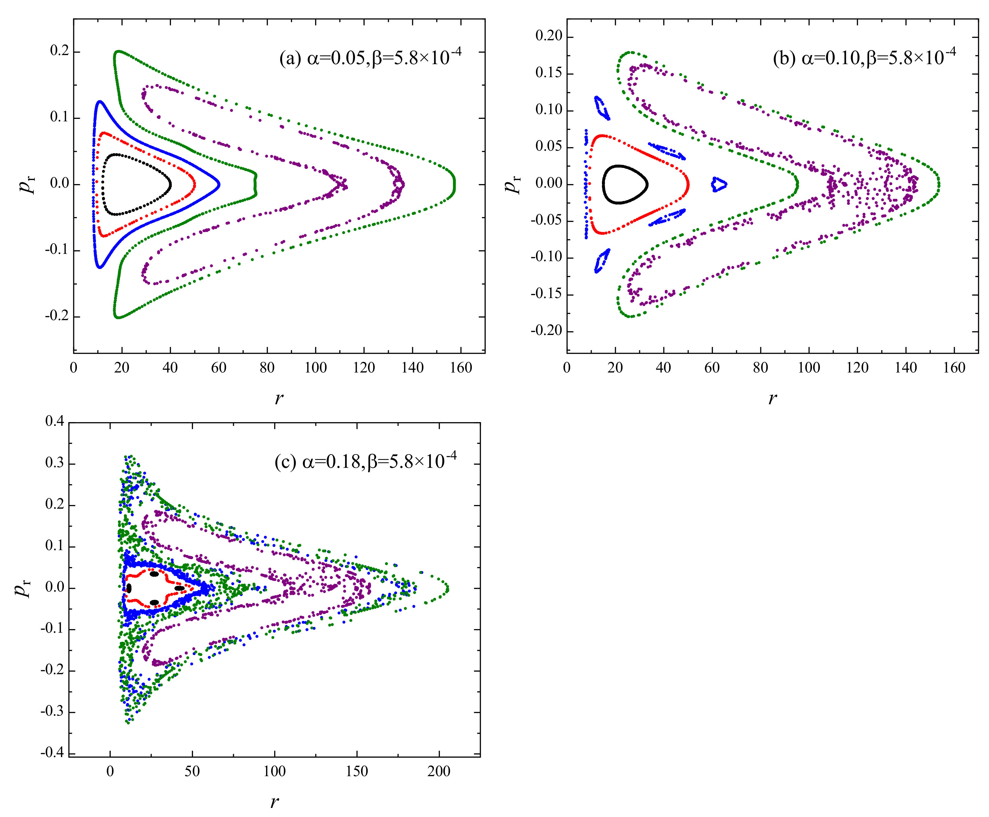
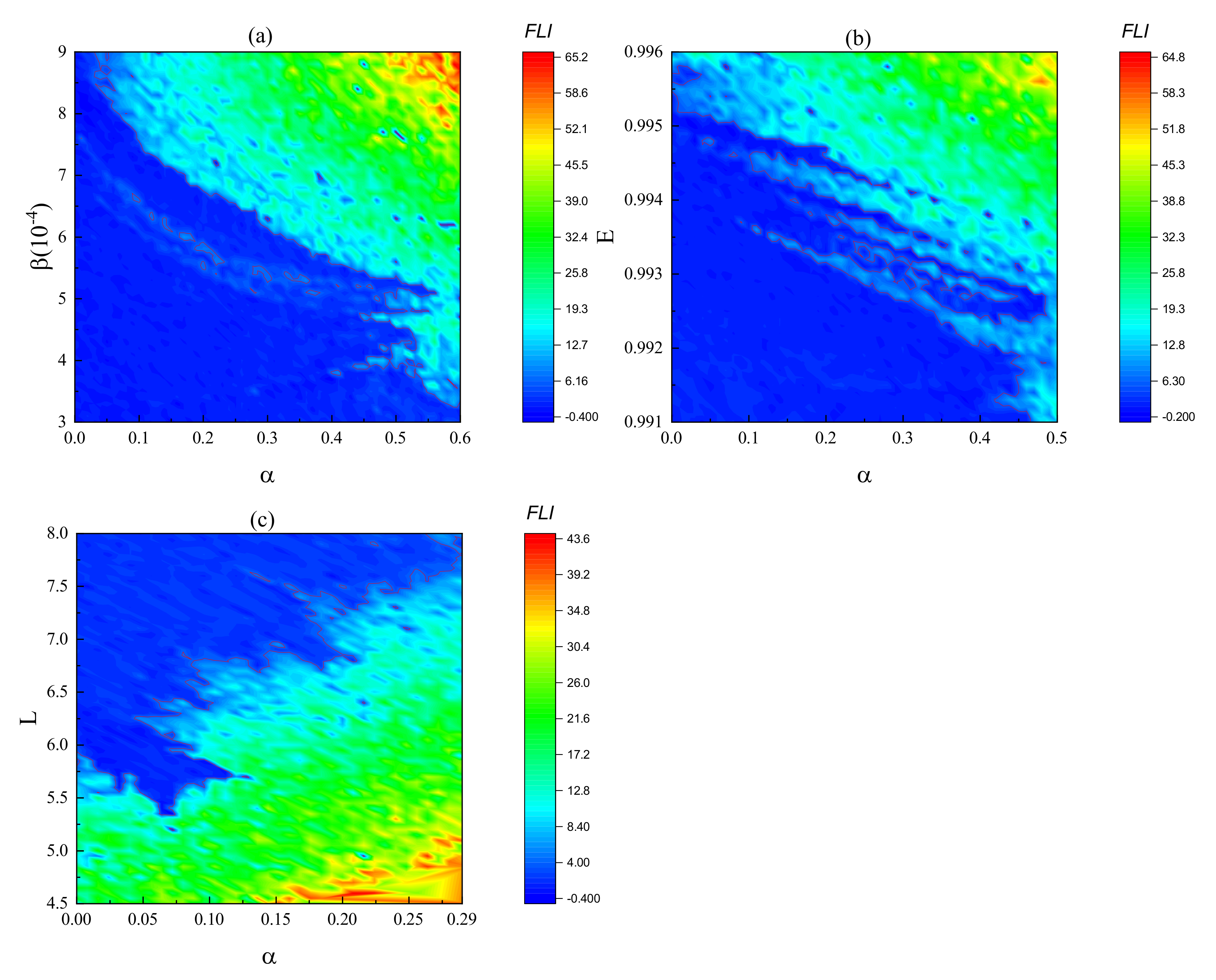
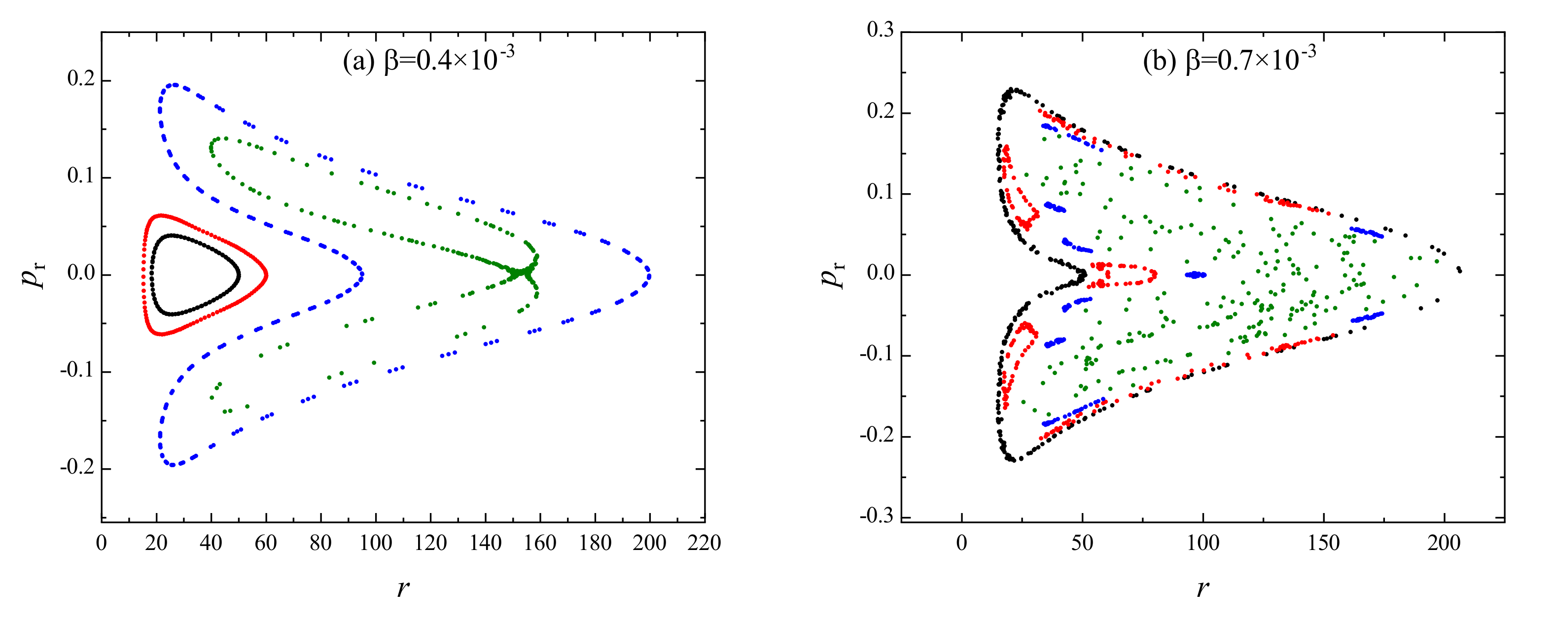
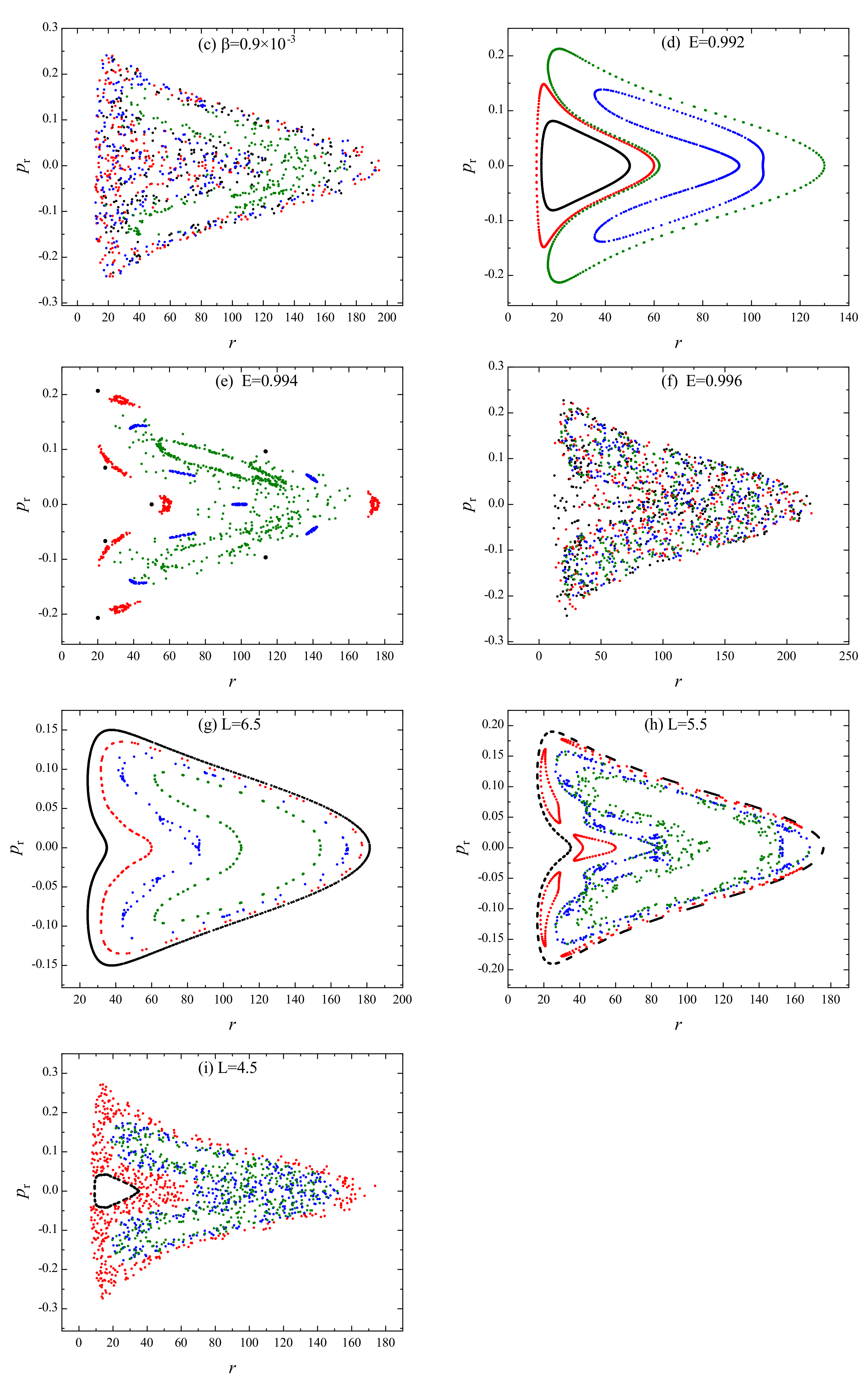
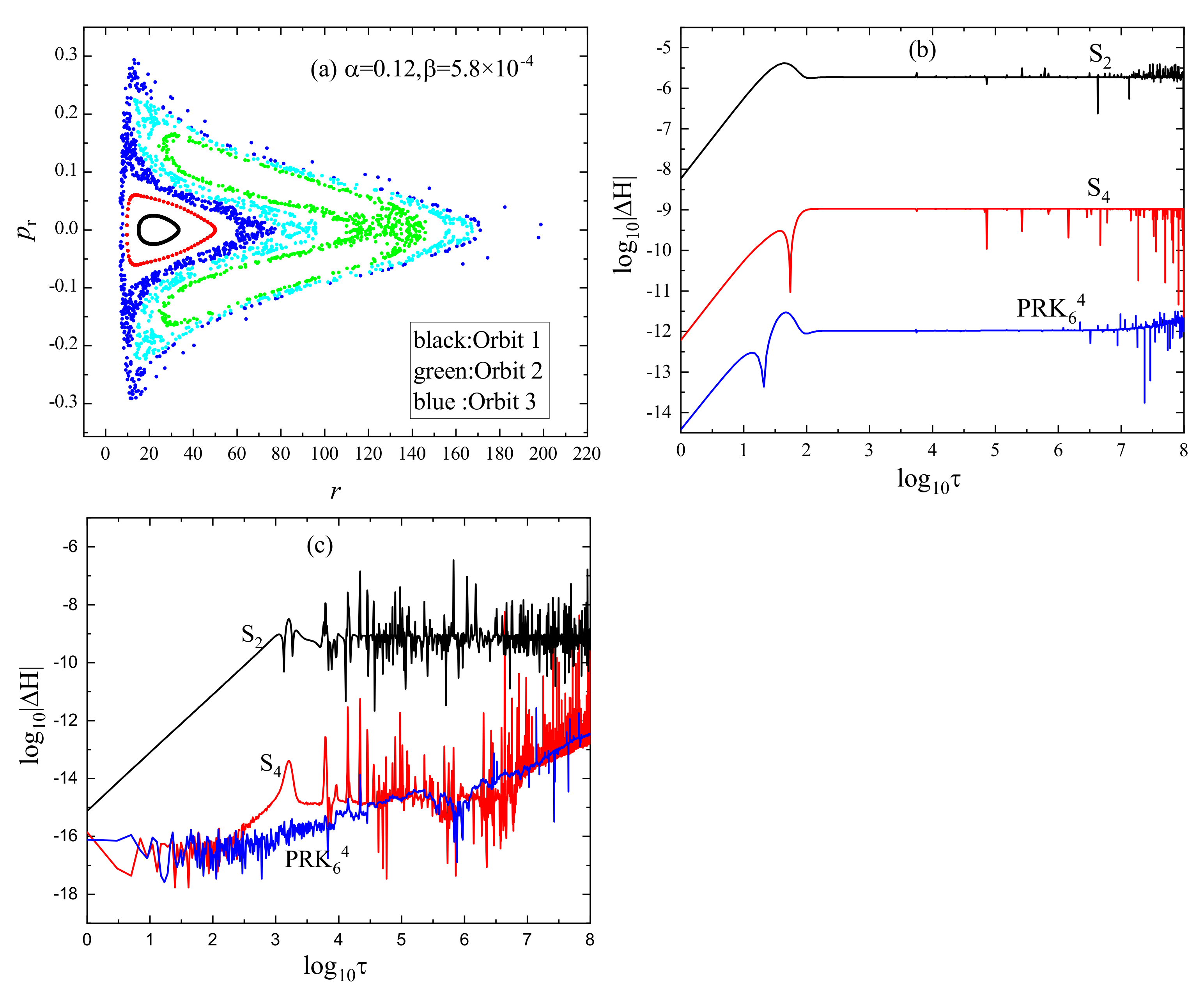
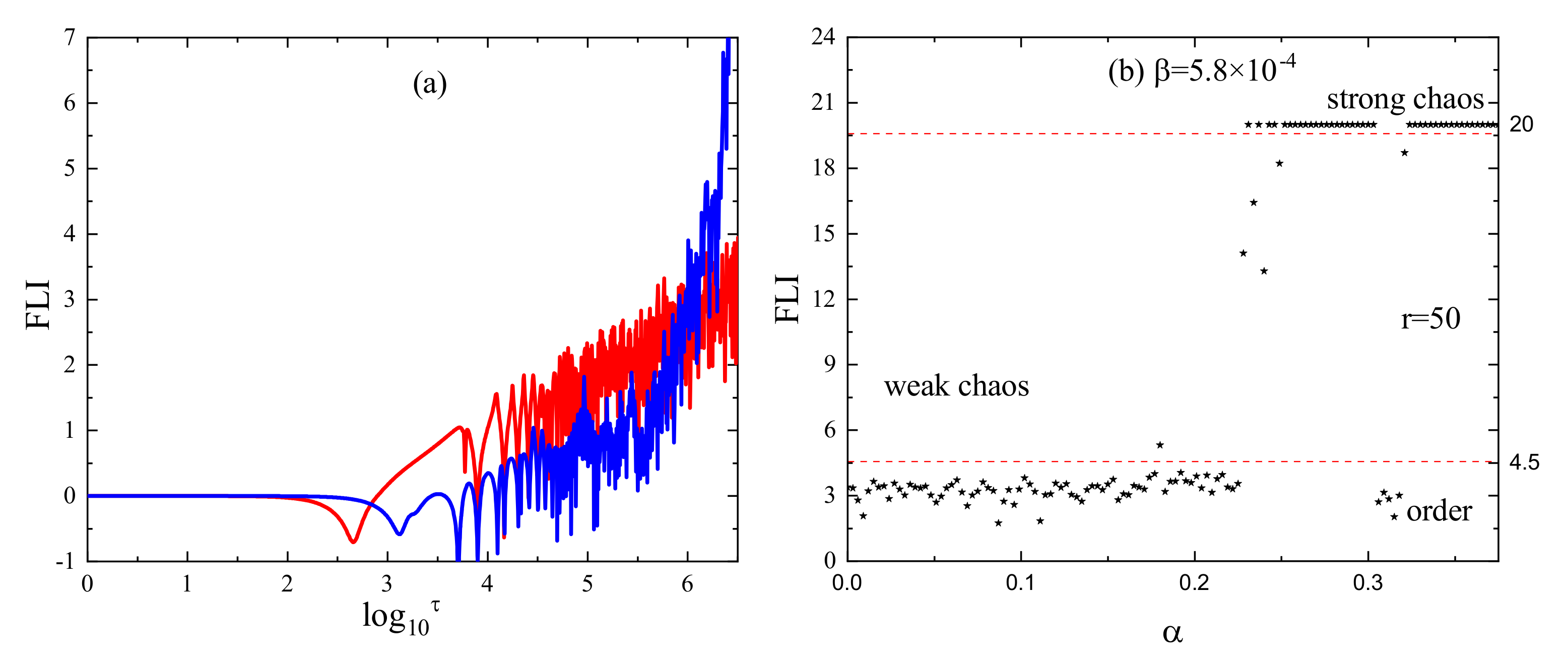
3.2. Orbital Dynamical Behavior

Figure 2 plots the Poincaré sections when several different values are given to the modified gravity parameter α . Orbit 2 with the initial separation r = 110 that is chaotic in Figure 1a is still chaotic for α = 0.05 in Figure 2a, α = 0.1 in Figure 2b and α = 0.18 in Figure 2c. We also show a path for Orbit 3 with the initial separation r = 60 in Figure 1a going from order to chaos as α increases. This orbit evolves from one single torus for α = 0.05 in Figure 2a to six islands for α = 0.1 in Figure 2b, and to chaos for α = 0.12 in Figure 1a and α = 0.18 in Figure 2c. Seen from the global phase space structures in Figure 1a and Figure 2, an increase of α leads to more orbits with stronger chaoticity. This does not mean that a given orbit always becomes stronger and stronger chaos in this case.
The regularity of Orbit 1 and the chaoticity of Orbit 2 in Figure 1a can also be identified in terms of the technique of fast Lyapunov indicator (FLI) in Figure 3a. The FLI with two nearby orbits is defined in [41,42] as a spacetime coordinate independent indicator:
FLI = log 10 d ( τ ) d ( 0 ) ,
where d ( 0 ) is the initial proper distance between two nearby orbits and d ( τ ) is a proper distance at the proper time τ . The FLI of Orbit 1 increasing in a power law with time log 10 τ shows the regularity of bounded Orbit 1. The FLI of Orbit 2 increasing in an exponential law with time indicates the chaoticity of bounded Orbit 2. It is found that ordered orbits correspond to the FLIs not more than 4.5 and chaotic orbits correspond to the FLIs larger than 4.5 when the integration time τ = 10 6 . With the aid of FLIs, the values of α can be classified according to the regular and chaotic two cases. In Figure 3b, the values of α < 0.178 correspond to order, and the values of 0.225 < α < 0.306 or α > 0.32 correspond to chaos.
The method of FLIs is used to find chaos by scanning one parameter space in Figure 3. This operation is still useful by scanning two parameter spaces. Figure 4a plots the regions of ( α , β ) for order and those for chaos. It is shown that the chaoticity is strengthened when α and β increase. This result is also supported by the method of Poincaré sections in Figure 5a–c. Similarly, chaos becomes stronger with an increase of E, as shown in Figure 4b and Figure 5d–f. However, chaos is weakened when L increases in Figure 4c and Figure 5g–i.
In short, chaos is strengthened from the global phase space structures when each of the modified gravity parameter α , the magnetic field parameter β and the particle energy E increases. However, it is weakened as the particle angular momentum L increases. Here, an explanation is given to these results. The analysis is based on Equation (12) with several main terms:
H 1 E 2 + L β 2 E 2 r ( 1 + α ) + E 2 2 r 2 α ( 1 + α ) + β 2 8 r 2 sin 2 θ + L 2 2 r 2 sin 2 θ + .
The expression is considered when 2 ( 1 + α ) / r 1 and α ( 1 + α ) / r 2 1 . The second term in Equation (23) corresponding to the second term of Equation (2) acts as the black hole gravity to the particle. Here, the modified gravity parameter α also plays a role in enhancing the gravitational effect. However, α in the third term of Equation (23) corresponding to the third term of Equation (2) gives a gravitational repulsive force contribution to the particle. The gravitational force from α in the second term of Equation (23) is more important than the gravitational repulsive force from α in the third term of Equation (23). The fourth term in Equation (23) corresponds to a magnetic field force as a gravitational effect. The fifth term corresponds to an inertial centrifugal force from the particle angular momentum. When anyone of the three parameters α , β and E increases, the gravitational effects are strengthened and the particle motions have more dramatic changes. As a result, chaos would become stronger from the global phase space structures when chaos can occur. On the contrary, an increase of the angular momentum leads to enlarging the repulsive force effects; equivalently, it weakens the gravitational effects and decreases the strength of chaos.

4. Conclusions

With the aid of the scalar–tensor–vector modified gravitational theory, the modified gravity Schwarzschild black hole was obtained in the literature through a modified gravity parameter. This parameter plays an important role in enhancing the gravitational constant and providing the black hole charge with a gravitational repulsive force contribution. The modified Schwarzschild black hole is still a static spherically symmetric black hole solution of the field equation. When the black hole is immersed in an external asymptotic uniform magnetic field, the dynamics of charged particles moving in the background field is not integrable.
Although the Hamiltonian for the description of the charged particle dynamics is inseparable to the variables, it still allows for the acceptance of explicit symplectic integrators because the Hamiltonian has five splitting parts with analytical solutions as explicit functions of proper time. Numerical tests show that the explicit symplectic integrators exhibit good performance in the long-term conservation of energy integral when appropriate time steps are chosen.
One of the explicit symplectic integrators combined with the techniques of Poincaré sections and fast Lyapunov indicators is mainly used to survey the effect of the modified gravity parameter on the regular and chaotic dynamical features of charged particle orbits. It is shown that chaos is strengthened from the global phase space structures under some circumstances as the modified gravity parameter increases. Such a similar result is also suitable for the case of the magnetic field parameter and the particle energy increasing. However, chaos is somewhat weakened with an increase of the particle angular momentum.

Author Contributions

Software and writing—original draft, D.Y.; software, W.C.; formal analysis, N.Z.; investigation, H.Z.; resources, W.L.; supervision, conceptualization, methodology, writing—review and editing and funding acquisition, X.W. All authors have read and agreed to the published version of the manuscript.

Funding

This research has been supported by the National Natural Science Foundation of China (Grant Nos. 11973020 and 11533004), and the Natural Science Foundation of Guangxi (Grant No. 2019JJD110006).

Institutional Review Board Statement

Not applicable.

Informed Consent Statement

Not applicable.

Data Availability Statement

Our paper is a theoretical work. All of the data are calculated and given in the paper.

Acknowledgments

The authors are very grateful to the referees for useful suggestions.

Conflicts of Interest

The authors declare no conflict of interest.

References

  1. Abbott, B.P.; Abbott, R.; Abbott, T.D.; Abernathy, M.R.; Acernese, F.; Ackley, K.; Adams, C.; Adams, T.; Addesso, P.; Adhikari, R.X.; et al. Observation of Gravitational Waves from a Binary Black Hole Merger. Phys. Rev. Lett. 2016, 116, 061102. [Google Scholar] [CrossRef]
  2. Abbott, R.; Abbott, T.D.; Abraham, S.; Acernese, F.; Ackley, K.; Adams, C.; Adhikari, R.X.; Adya, V.B.; Affeldt, C.; Agathos, M.; et al. Properties and Astrophysical Implications of the 150 M Binary Black Hole Merger GW190521. Astrophys. J. Lett. 2020, 900, L13. [Google Scholar] [CrossRef]
  3. The Event Horizon Telescope Collaboration; Akiyama, K.; Alberdi, A.; Alef, W.; Asada, K.; Azulay, R.; Baczko, A.-K.; Ball, D.; Baloković, M. First M87 Event Horizon Telescope Results. I. The Shadow of the Supermassive Black Hole. Astrophys. Lett. 2019, 875, L1. [Google Scholar] [CrossRef]
  4. Clifton, T.; Ferreira, P.F.; Padilla, A.; Skordis, C. Modified gravity and cosmology. Phys. Rep. 2012, 513, 1–189. [Google Scholar] [CrossRef] [Green Version]
  5. Russo, J.G.; Tseytlin, A.A. Scalar-tensor quantum gravity in two dimensions. Nucl. Phys. B 1992, 382, 259–275. [Google Scholar] [CrossRef] [Green Version]
  6. Deng, X.-M. Geodesics and periodic orbits around quantum-corrected black holes. Phys. Dark Universe 2020, 30, 100629. [Google Scholar] [CrossRef]
  7. Deng, X.-M. Periodic orbits around brane-world black holes. Eur. Phys. J. C 2020, 80, 489. [Google Scholar] [CrossRef]
  8. Zhou, T.-Y.; Xie, Y. Precessing and periodic motions around a black-bounce/traversable wormhole. Eur. Phys. J. C 2020, 80, 1070. [Google Scholar] [CrossRef]
  9. Zhang, J.; Xie, Y. Probing a self-complete and Generalized-Uncertainty-Principle black hole with precessing and periodic motion. Astrophys. Space Sci. 2022, 367, 17. [Google Scholar] [CrossRef]
  10. Strominger, A.; Trivedi, S.P. Information consumption by Reissner-Nordström black holes. Phys. Rev. D 1993, 48, 5778–5783. [Google Scholar] [CrossRef] [Green Version]
  11. Kazakov, D.I.; Solodukhin, S.N. On quantum deformation of the Schwarzschild solution. Nucl. Phys. B 1994, 429, 153–176. [Google Scholar] [CrossRef] [Green Version]
  12. Lin, H.-Y.; Deng, X.-M. Rational orbits around 4D Einstein-Lovelock black holes. Phys. Dark Universe 2021, 31, 100745. [Google Scholar] [CrossRef]
  13. Gao, B.; Deng, X.-M. Dynamics of charged test particles around quantum-corrected Schwarzschild black holes. Eur. Phys. J. C 2021, 81, 983. [Google Scholar] [CrossRef]
  14. Lin, H.-Y.; Deng, X.-M. Precessing and periodic orbits around Lee-Wick Black holes. Eur. Phys. J. Plus 2022, 137, 176. [Google Scholar] [CrossRef]
  15. Lin, H.-Y.; Deng, X.-M. Bound orbits and epicyclic motions around renormalization group improved Schwarzschild black holes. Universe 2022, 8, 278. [Google Scholar] [CrossRef]
  16. Nordstrom, G. On the possibility of unifying the electromagnetic and the gravitational fields. Phys. Z. 1914, 15, 504–506. [Google Scholar]
  17. Deng, X.-M.; Xie, Y. Improved upper bounds on Kaluza-Klein gravity with current Solar System experiments and observations. Eur. Phys. J. C 2015, 75, 539. [Google Scholar] [CrossRef] [Green Version]
  18. Bergmann, P.G. Comments on the scalar tensor theory. Int. J. Theor. Phys. 1968, 1, 25–36. [Google Scholar] [CrossRef]
  19. Deng, X.-M. Constraints on a scalar-tensor theory with an intermediate-range force by binary pulsars. Sci. China Phys. Mech. Astron. 2011, 54, 2071–2077. [Google Scholar] [CrossRef]
  20. Deng, X.-M.; Xie, Y. Two-post-Newtonian light propagation in the scalar-tensor theory: An N-point mass case. Phys. Rev. D 2012, 86, 044007. [Google Scholar] [CrossRef] [Green Version]
  21. Deng, X.-M. Two-post-Newtonian approximation of the scalar-tensor theory with an intermediate-range force for general matter. Sci. China Phys. Mech. Astron. 2015, 58, 030002. [Google Scholar] [CrossRef]
  22. Deng, X.-M.; Xie, Y. Solar System tests of a scalar-tensor gravity with a general potential: Insensitivity of light deflection and Cassini tracking. Phys. Rev. D 2016, 93, 044013. [Google Scholar] [CrossRef]
  23. Cheng, X.-T.; Xie, Y. Probing a black-bounce, traversable wormhole with weak deflection gravitational lensing. Phys. Rev. D 2021, 103, 064040. [Google Scholar] [CrossRef]
  24. Jacobson, T. Einstein-aether gravity: A status report. arXiv 2007, arXiv:0801.1547. [Google Scholar]
  25. Rosen, N. A bi-metric theory of gravitation. Gen. Relativ. Gravit. 1973, 4, 435–447. [Google Scholar] [CrossRef]
  26. Nojiri, S.; Odintsov, S.D. Modified f(R) gravity consistent with realistic cosmology: From a matter dominated epoch to a dark energy universe. Phys. Rev. D 2006, 74, 086005. [Google Scholar] [CrossRef] [Green Version]
  27. Nojiri, S.; Odintsov, S.D.; Oikonomou, V.K. Modified gravity theories on a nutshell: Inflation, bounce and late-time evolution. Phys. Rep. 2017, 692, 1–104. [Google Scholar] [CrossRef] [Green Version]
  28. Deng, X.-M. Probing f(T) gravity with gravitational time advancement. Class. Quantum Gravity 2018, 35, 175013. [Google Scholar] [CrossRef]
  29. Moffat, J.W. Scalar tensor vector gravity theory. J. Cosmol. Astropart. Phys. 2006, 3, 4. [Google Scholar] [CrossRef]
  30. Deng, X.-M.; Xie, Y.; Huang, T.-Y. Modified scalar-tensor-vector gravity theory and the constraint on its parameters. Phys. Rev. D 2009, 79, 044014. [Google Scholar] [CrossRef] [Green Version]
  31. Moffat, J.W.; Rahvar, S. The MOG weak field approximation and observational test of galaxy rotation curves. Mon. Not. R. Astron. Soc. 2013, 436, 1439–1451. [Google Scholar] [CrossRef] [Green Version]
  32. Moffat, J.W.; Rahvar, S. The MOG Weak Field approximation II. Observational test of Chandra X-ray Clusters. Mon. Not. R. Astron. Soc. 2013, 441, 3724–3732. [Google Scholar] [CrossRef] [Green Version]
  33. Moffat, J.W. Black holes in modified gravity (MOG). Eur. Phys. J. C 2015, 75, 175. [Google Scholar] [CrossRef]
  34. Haydarov, K.; Rayimbaev, J.; Abdujabbarov, A.; Palvanov, S.; Begmatova, D. Magnetized particle motion around magnetized Schwarzschild-MOG black hole. Eur. Phys. J. C 2020, 80, 399. [Google Scholar] [CrossRef]
  35. Haydarov, K.; Boboqambarova, M.; Turimov, B.; Abdujabbarov, A.; Akhmedov, A. Circular motion of particle around Schwarzschild-MOG black hole. arXiv 2021, arXiv:2110.05764. [Google Scholar]
  36. Moffat, J.W. Modified gravity black holes and their observable shadows. Eur. Phys. J. C 2015, 75, 130. [Google Scholar] [CrossRef]
  37. Wang, Y.; Sun, W.; Liu, F.; Wu, X. Construction of Explicit Symplectic Integrators in General Relativity. II. Reissner-Nordström Black Holes. Astrophys. J. 2021, 909, 22. [Google Scholar] [CrossRef]
  38. Yoshida, H. Construction of higher order symplectic integrators. Phys. Lett. A 1990, 150, 262. [Google Scholar] [CrossRef]
  39. Blanes, S.; Moan, P.C. Practical symplectic partitioned Runge-Kutta and Runge-Kutta-Nyström methods. J. Comput. Appl. Math. 2002, 142, 313. [Google Scholar] [CrossRef] [Green Version]
  40. Zhou, N.; Zhang, H.; Liu, W.; Wu, X. A Note on the Construction of Explicit Symplectic Integrators for Schwarzschild Spacetimes. Astrophys. J. 2022, 927, 160. [Google Scholar] [CrossRef]
  41. Froeschlé, C.; Lega, E. On the Structure of Symplectic Mappings. The Fast Lyapunov Indicator: A Very Sensitive Tool. Celest. Mech. Dyn. Astron. Vol. 2000, 78, 167–195. [Google Scholar] [CrossRef]
  42. Wu, X.; Huang, T.Y.; Zhang, H. Lyapunov indices with two nearby trajectories in a curved spacetime. Phys. Rev. D 2006, 74, 083001. [Google Scholar] [CrossRef] [Green Version]
Figure 1. (a) Poincaré sections at the plane θ = π / 2 with p θ > 0 , where the phase space structures are described by the algorithm S 2 with the proper step h = 1 . The parameters are E = 0.995 , L = 4.6 , α = 0.12 and β = 5.8 × 10 4 . The initial conditions are p r = 0 and θ = π / 2 . Orbit 1 with the initial separation r = 15 is a closed regular curve, and Orbit 2 with the initial separation r = 110 is chaotic. Orbit 3 with the initial separation r = 60 is also chaotic. (b) Hamiltonian errors Δ H = H + 1 / 2 for the three symplectic methods acting on the ordered Orbit 1. The error for S 4 is about three orders of magnitude smaller than for S 2 , but larger than for P R K 6 4 . (c) Hamiltonian errors Δ H = H + 1 / 2 for the three symplectic methods acting on the chaotic Orbit 2. Although S 4 and P R K 6 4 have higher accuracies than S 2 in an integration time, they would approach S 2 in secular error behavior due to roundoff errors.
Universe 08 00320 g001
Figure 2. Poincaré sections for three values of the modified gravity coupling parameter, where α = 0.05 in (a), α = 0.1 in (b) and α = 0.18 in (c). The other parameters are E = 0.995 , L = 4.6 and β = 5.8 × 10 4 . It is shown via the three panels that chaos gets stronger with α increasing.
Universe 08 00320 g002
Figure 3. (a) Fast Lyapunov indicators (FLIs) for Orbits 1 and 2 in Figure 1a. The FLI grows slowly with time for the ordered orbit 1 (colored Red), but quickly for the chaotic orbit 2 (colored Blue). (b) Dependence of FLI on the modified gravity parameter α . The other parameters are the same as those of Orbit 1, and the initial separation is r = 50 . Each value of the FLIs is obtained after the integration time reaches τ = 1 × 10 6 ; 4.5 is a threshold value of the FLIs between order and chaos. The FLIs smaller than (or equal to) this threshold show the regularity. However, the FLIs more than this threshold indicate the chaoticity. In this way, the values of α corresponding to order and those corresponding to chaos are clearly listed in this figure.
Universe 08 00320 g003
Figure 4. Distributions of two parameters corresponding to order and chaos in terms of FLIs. The initial radius is r = 110 . (a) Distributions of α and β . The other parameters are E = 0.995 and L = 6 . (b) Distributions of α and E. The other parameters are β = 7.8 × 10 4 and L = 6 . (c) Distributions of α and L. The other parameters are β = 7.8 × 10 4 and E = 0.995 . These figures show that chaos becomes stronger as α , β and E increase or L decreases.
Universe 08 00320 g004
Figure 5. Poincaré sections. (ac): Three different values are given to β . The modified gravity coupling parameter is α = 0.3 , and the other parameters are consistent with those of Figure 4a. (df): Three different values are given to E. The modified gravity coupling parameter is α = 0.3 , and the other parameters are those of Figure 4b. (gi): Three different values are given to L. The modified gravity coupling parameter is α = 0.05 , and the other parameters are those of Figure 4c.
Universe 08 00320 g005aUniverse 08 00320 g005b
Publisher’s Note: MDPI stays neutral with regard to jurisdictional claims in published maps and institutional affiliations.

