Effects of a Finite Volume in the Phase Structure of QCD

Abstract

Working in the SU(2) flavor version of the NJL model, we study the effect of taking a finite system volume on a strongly interacting system of quarks, and, in particular, the location of the chiral phase transition and the CEP. We consider two shapes for the volume, spherical and cubic regions with different sizes and different boundary conditions. To analyze the QCD phase diagram, we use a novel criterion to study the crossover zone. A comparison between the results obtained from the two different shapes and several boundary conditions is carried out. We use the method of Multiple Reflection Expansion to determine the density of states and three kinds of boundary conditions over the cubic shape. These boundary conditions are: periodic, anti-periodic and stationary boundary conditions on the quark fields.

1. Introduction

Two of the most interesting aspects of Quantum Chromodynamics (QCD) are the chiral symmetry breaking and the deconfinement phenomena. Today, we know that the meson isospin structure in the light sector we observe in nature is a direct consequence of both the spontaneous and the explicit chiral symmetry breaking [1,2]. On the other hand, deconfinement is still not fully understood [3,4], and many theoretical and experimental efforts are currently being made to understand it better [5]. One intuitive way to present these phenomena with different system boundary conditions is via a QCD phase diagram, as there is a common agreement about the dependence of the chiral symmetry and confinement on the system temperature [6,7,8,9] and, to a lesser extent, on the chemical potential [10,11].

Chiral symmetry is a fundamental concept in the explanation of the existence of baryonic mass. The spontaneous breaking of the chiral symmetry is best exemplified by the existence of an isospin triplet state portrayed by the three pi mesons (${\pi }^{+}$, ${\pi }^{-}$ and ${\pi }^0$) which correspond to the (pseudo) Goldstone bosons for the approximate SU(2) flavor symmetry. This mechanism is of utmost importance, as nearly all the mass that can be measured in the observable universe exists because of this. During the evolution of the universe, from the Big Bang until today, the underlying exact and approximate symmetries that strongly interacting particles possess are fundamental for our understanding of the inner workings of nature.

Confinement was one of the most important features during the progress of the universe just moments after the Big Bang [12,13,14] although it is unknown how (or if) the baryon asymmetry of the universe affected the general state (specifically the chemical potential) of the early universe [15,16,17,18]. In the QCD phase diagram, this general state of the early universe is described in the high temperature and either the zero or low nonzero chemical potential zone. If the baryon asymmetry did not take a role whatsoever, then the chemical potential was exactly zero. Today, we think that a deconfined state of matter which we call quark gluon plasma (QGP) existed in the earliest moments of the universe.

Another natural instance where the confinement takes an important role is in the description of the nucleus and the inner layers of the neutron stars [19,20,21,22]. Strongly interacting matter is thought to be so tightly packed in these stars that the regular atomic arrangement of matter becomes degenerate [23]. In the phase diagram, this kind of system is described in the low temperature and high chemical potential zone. This particular zone is also of special interest because many QCD-based models predict the existence of a critical end point (CEP) in this zone [24,25,26]. A CEP is a point in the temperature–chemical potential plane where a first order phase transition ends and a continuous but complete shift of the order parameter, called a crossover, starts.

Currently, many theoretical and experimental efforts are being made to gain more knowledge about the QCD phase diagram. Lattice QCD is a method that takes first principles as a starting point; however, at present, there are several nontrivial difficulties at nonzero chemical potentials with lattice QCD with the sign problem [5,27,28,29]. Effective models such as the NJL type models, the QM type models, etc., sacrifice the gauge symmetry of QCD to obtain a plausible description of several aspects of QCD at nonzero chemical potentials. For physical values of the quark masses and vanishing chemical potentials, lattice QCD predicts a rapid but smooth chiral crossover around the pseudocritical temperature $T_c\approx 155$ MeV [30,31,32]. Effective theories take this prediction as a starting point, but they are not forced to agree with each other with the qualitative aspects of the QCD phase diagram at finite chemical potential [24,33]. Experimentally, many ultra-relativistic heavy ion collisions performed at the LHC [34,35], RHIC [36], NICA [37], SPS [38], NA61/SHINE [39] and many other research centers can give insight about the QCD phase diagram itself.

In this work, we study the QCD phase diagram in the framework of the two-flavor Nambu–Jona–Lasinio model, but we consider a system outside of the thermodynamic limit to be limited within a finite volume. We decided to work in the $SU\left(2\right)$ version of the NJL model to keep the computation difficulties of the resulting phase diagrams at a bare minimum. In the current experimental work, heavy ion collisions are being performed, where a QGP state is thought to be able to be achieved [40,41,42] although the volume this state occupies is very small and lasts for a very limited timespan until it reaches freeze-out. This volume can be considered in theoretical calculations as having different sizes and geometries. Frequently, the consideration of a finite volume to study its effects in the QCD phase diagram has been carried out by contemplating a cubic box [43,44,45,46], and very few of the studies have considered the spherical shape [47,48] which is more realistic. In our work, we consider spherical and cubic droplets with density of states derived from the Multiple Reflection Expansion (MRE). In addition, we work within a cubic box of finite size L comparing boundary conditions: stationary wave, periodic and antiperiodic.

2. Two-Flavor Nambu–Jona–Lasinio (NJL) Model

The four-quark point interaction in the NJL model is described by the Lagrangian [49]

$$\begin{array}{c}\hfill \mathcal{L}=\overline{q}\left(i\cancel{\partial }-{\widehat{m}}_0\right)q+{\displaystyle \frac{G}{2}}\left[{\left(\overline{q}q\right)}^2+{\left(\overline{q}i{\gamma }_5\mathit{\tau }q\right)}^2\right],\end{array}$$

(1)

where $\cancel{\partial }={\gamma }^{\mu }{\partial }_{\mu }$, $q={\left(q_u,q_d\right)}^T$ denotes the quark field in the fundamental representation of the flavor SU(2), and ${\widehat{m}}_0=\mathrm{diag}\left(m_u,m_d\right)$ stands for the current quark mass matrix. We assume exact isospin symmetry, namely $m_0=m_u=m_d$. $\mathit{\tau }$ are the Pauli matrices, and G is the coupling constant.

In the chiral limit, the NJL model describes the dynamical chiral symmetry breaking of $SU{\left(2\right)}_L\otimes SU{\left(2\right)}_R$ down to $SU{\left(2\right)}_V$ symmetry [50]. As a result, the quark–antiquark pairing gives rise to the chiral condensate $⟨\overline{q}q⟩$ with nonzero expectation value [51,52]. Accordingly, the order parameter is $⟨\overline{q}q⟩=⟨{\overline{q}}_R{q}_L+{\overline{q}}_L{q}_R⟩\sim \sigma$ [53,54], where $\sigma$ is the mesonic field corresponding to the expectation value $⟨\overline{q}q⟩$. In nature, a finite current quark mass breaks the chiral symmetry explicitly. In the mean field approximation, the constituent quark mass is related to the chiral condensate through the self-consistent gap Equation [55,56,57]

$$M=m_0-\sigma =m_0-G⟨\overline{q}q⟩.$$

(2)

In a vacuum, the condensation

$$⟨\overline{q}q⟩=-\int \frac{{\mathrm{d}}^{4}p}{{(2\pi )}^4}\mathrm{tr}\left[S\left(p\right)\right],$$

(3)

where $S\left(p\right)$ is the dressed quark propagator

$$S\left(p\right)=\frac{{\gamma }^{\mu }{p}_{\mu }+M}{p^2-M^2},$$

(4)

and the trace is taken in color, flavor and Dirac spinor spaces. In the gap Equation (2), the two remaining free parameters are the (finite) temperature (T) and the chemical potential ($\mu$), so this equation can be solved self-consistently for any two given values of T and $\mu$ to obtain a description of the thermodynamic state at those conditions. To study the thermodynamic properties of the system at a determined region in the $T-\mu$ plane, we work with the thermodynamic potential per unit volume [58] in the imaginary time formalism. We perform a Wick rotation $t\to \tau =it,t=-i\tau$, and the temperature and chemical potential are introduced by means of [59,60]

$$i\int \frac{d^{4}p}{{(2\pi )}^4}f(p_0,\mathit{p})\to -T\sum _{-\infty }^{\infty }\int \frac{{\mathrm{d}}^3\mathit{p}}{{(2\pi )}^3}f(i{\omega }_n-\mu ,\mathit{p}),$$

(5)

where $p_0\to i{p}_0={\omega }_n,p_0=-i{\omega }_n$, ${\omega }_n=(2n+1)\pi T$ are the Matsubara frequencies for fermions. Thus we have

$$\mathsf{\Omega }(T,\mu )=\frac{{\sigma }^2}{2G}-T\sum _n\int \frac{{\mathrm{d}}^3\mathit{p}}{{(2\pi )}^3}\mathrm{tr}\left[ln\frac{S^{-1}(i{\omega }_n,\mathit{p})}{T}\right],$$

(6)

and the inverse quark propagator in momentum space is defined as [55,61]

$$S^{-1}(p_0,\mathit{p})={\gamma }_0(p^0+\mu )-\gamma ·\mathit{p}-M,$$

(7)

computing the trace through the identity $\mathrm{tr}lnX=ln\det \left(X\right)$, we obtain

$$\mathsf{\Omega }(T,\mu )=\frac{{\sigma }^2}{2G}-2N_c{N}_f\int \frac{{\mathrm{d}}^3\mathit{p}}{{(2\pi )}^3}\left\{E_{\mathit{p}}+Tln[Z^{+}\left(E_{\mathit{p}}\right)]+Tln\left[Z^{-}\left(E_{\mathit{p}}\right)\right]\right\},$$

(8)

where $E_{\mathit{p}}=\sqrt{{\mathit{p}}^2+M^2}$ is the energy of quarks, $N_c$ is the number of colors and $N_f$ is the number of flavors. The fermionic partition function is then given by

$$Z^{\pm }\left(E_{\mathit{p}}\right)=1+e^{[-\beta (E_{\mathit{p}}\mp \mu )]}.$$

(9)

To describe the system at finite temperature and chemical potential and to analyze the behavior of $⟨\overline{q}q⟩$, the thermodynamic potential (8) is minimized. One way to include the finite volume effects is by using a modified density of states derived from the multiple reflection expansion (MRE) [62,63,64]. In this model, we consider a sphere of radius R that encloses a quark matter system. The density of states per unit volume in the (MRE) for a sphere at first order is given by [65,66]

$${\rho }_{MRE}={\displaystyle \frac{p^2}{2{\pi }^2}}\left[1+{\displaystyle \frac{6{\pi }^2}{pR}}{f}_S\left(\frac{p}{\alpha }\right)+{\displaystyle \frac{12{\pi }^2}{{\left(pR\right)}^2}}{f}_C\left(\frac{p}{\alpha }\right)\right],$$

(10)

where

$$\begin{array}{cc}\hfill f_S\left(\frac{p}{\alpha }\right)& \hfill =-\frac{1}{8\pi }\left[1-\frac{2}{\pi }arctan\frac{p}{\alpha }\right],\hfill \end{array}$$

(11)

$$\begin{array}{cc}\hfill f_C\left(\frac{p}{\alpha }\right)& \hfill =\frac{1}{12{\pi }^2}\left[1-\frac{3p}{2\alpha }\left(\frac{\pi }{2}-arctan\frac{p}{\alpha }\right)\right],\hfill \end{array}$$

(12)

are the the surface and curvature contributions to the density of states, respectively. The parameter $\alpha$ is related to the penetration of the wave function of the quark matter confined in a finite volume into the hadronic medium [67].

As Equation (10) is quadratic in p, two real roots are bound to appear in the density of states. If they do, that would imply that the density of states, which has a positive quadratic coefficient, is negative between these roots. These negative density values are unphysical, so an infrared (IR) cutoff ${\Lambda }_{IR}$ is defined in momentum space. The following replacement is performed [64]

$$\int \frac{{\mathrm{d}}^3\mathit{p}}{{(2\pi )}^3}f(T,\mu ,\mathit{p})\to {\int }_0^{\infty }\mathrm{d}p\rho \left(p\right)f(T,\mu ,p)\to {\int }_{{\Lambda }_{IR}}^{{\Lambda }_{UV}}\mathrm{d}p{\rho }_{MRE}(p,\alpha ,R)f(T,\mu ,p),$$

(13)

where ${\Lambda }_{IR}$ is the largest solution to ${\rho }_{MRE}(p,\alpha ,R)=0$ with respect to momentum p.

The NJL model is a non-renormalizable effective model that leads to divergent integrals [68,69], so we need to introduce a regularization procedure. A relatively simple regularization method is achieved by adding a three-momentum cut-off to the integrals to eliminate the ultraviolet divergences [70]. The momentum integrals are limited in the upper limit by ${\mathit{p}}^2={\Lambda }_{UV}^2$ [71], where ${\Lambda }_{UV}$ is the three-momentum cutoff.

Following [72,73], the Dirichlet boundary condition is imposed by setting $\alpha =\infty$ in (11) and (12). The density of states [Equation (10)] takes the form:

$$\begin{array}{c}\hfill {\rho }_{MRE}={\displaystyle \frac{p^2}{2{\pi }^2}}\left[1-{\displaystyle \frac{3\pi }{4pR}}+{\displaystyle \frac{1}{{\left(pR\right)}^2}}\right].\end{array}$$

(14)

where ${\Lambda }_{IR}=1.8/R$. On the other hand, to be consistent with the MIT Bag model, the Neumann boundary conditions are applied for $\alpha =0$ [72]. With this, the infrared cutoff becomes ${\Lambda }_{IR}=1/\sqrt{2}R$.

Nevertheless, the thermodynamic properties of a finite volume system depend not only on the size of the system, but also on its geometric shape [48]. Therefore, we also consider a cubic shape for the MRE approximation of the density of states. With this geometry, the curvature contribution to the density of states is zero. The obtained density of states is

$$\begin{array}{c}\hfill {\rho }_{MRE}={\displaystyle \frac{k^2}{2{\pi }^2}}\left(1-{\displaystyle \frac{3}{4kL}}\right),\end{array}$$

(15)

with these conditions ${\Lambda }_{IR}=0.75/L$.

Another way to analyze the finite volume effects is by considering the system as a cubic box with finite length L and working within a discrete three-momentum scheme introducing specific boundary conditions. Small volumes imply high frequency modes. Hence, a regularization scheme that includes the whole momentum spectra is needed. If a UV cutoff is adopted, the contribution of high frequency modes would be ignored, and if an infrared cutoff is applied, the contribution of low frequency modes would be ignored [57].

In this approximation, which is explained in greater detail in Appendix B, the proper time regularization is used. In the regularization, the integrand that appears on the gap Equation is adjusted with a regularization factor that vanishes when $p\to \infty$, which allows accounting for all relevant momenta. Under this scheme, the chiral condensate at vacuum is given by

$$⟨\overline{q}q⟩=-4M{N}_c{N}_{f}T{\int }_{{\tau }_{UV}}^{\infty }\mathrm{d}\tau e^{-\tau (M^2-{\mu }^2)}{\Theta }_2\left[-2\tau \pi T\mu ,e^{-4{\pi }^2{T}^2\tau }\right]\int {\displaystyle \frac{{\mathrm{d}}^3\mathit{p}}{{(2\pi )}^3}}{e}^{-\tau {\mathit{p}}^2},$$

(16)

where ${\Theta }_2\left[z,q\right]\equiv {\sum }_{n=-\infty }^{\infty }{q}^{{(n+1/2)}^2}{e}^{(2n+1)iz}$ is the Jacobi’s theta function. To modify the condensation, the integral over momentum is replaced with a sum over all allowed momentum modes [48,74]

$$\int {\displaystyle \frac{{\mathrm{d}}^3\mathit{p}}{{(2\pi )}^3}}\to \frac{1}{V}\sum _{\mathit{p}}$$

(17)

with V the volume of the system. The discrete momentum depending on the boundary conditions is

$$\sum _n{p}_{n,PBC}^2={\displaystyle \frac{4{\pi }^2}{L^2}}\sum _{n=-\infty }^{\infty }{n}^2,\sum _n{p}_{n,APBC}^2={\displaystyle \frac{4{\pi }^2}{L^2}}\sum _{n=-\infty }^{\infty }{\left(n+\frac{1}{2}\right)}^2,\sum _n{p}_{n,SWC}^2={\displaystyle \frac{{\pi }^2}{L^2}}\sum _{n=0}^{\infty }{n}^2,$$

(18)

Antiperiodic boundary conditions for fields in the Euclidean time direction are needed. In that manner, the anticommutation relations for fermions enclosed into a finite Euclidean box are satisfied [75,76]. However, in light of the fact that the Matsubara frequencies for fermions were used earlier (5), the boundary conditions for these frequencies in the imaginary time formalism are antiperiodic. For this reason, any boundary condition scheme between PBC and APBC for spatial directions is adequate to describe this finite volume system [74].

The zero-momentum mode contribution becomes especially important for small volume size. While APBC induces chiral symmetry restoration, PBC including the fermionic zero mode enhances the chiral condensate [75]. Stationary wave conditions in which the generated plasma is limited inside of a finite volume surrounded by a cold external medium were proposed by [44,77] to simulate the particle collision experiments performed in the laboratory. Therefore, the quark wave functions must be equal to zero in the boundaries.

By applying the conditions (18) on the chiral condensate (16), we obtain

$$⟨\overline{q}q⟩=-4M{N}_c{N}_{f}T{\int }_{{\tau }_{UV}}^{\infty }\mathrm{d}\tau e^{-\tau (M^2-{\mu }^2)}{\Theta }_2\left[-2\tau \pi T\mu ,e^{-4{\pi }^2{T}^2\tau }\right]{\left[\frac{f\left(\theta \right)}{L}\right]}^3$$

(19)

with

$$f\left(\theta \right)=\left\{\begin{array}{cc}{\Theta }_3\left[0,e^{-4{\pi }^2\tau /L^2}\right]\hfill & \mathrm{for}\mathrm{PBC}\hfill \\ {\Theta }_2\left[0,e^{-4{\pi }^2\tau /L^2}\right]\hfill & \mathrm{for}\mathrm{APBC}\hfill \\ \frac{1}{2}\left({\Theta }_3\left[0,e^{-{\pi }^2\tau /L^2}\right]-1\right)\hfill & \mathrm{for}\mathrm{SWC}\hfill \end{array}\right.$$

(20)

3. Setting Parameters

3.1. Multiple Reflection Expansion

For each symmetry and boundary condition, we obtained its corresponding set of parameters: ultraviolet three-momentum cutoff ${\Lambda }_{UV}$, infrared three-momentum cutoff ${\Lambda }_{IR}$ and the coupling strength constant G for $m_0=5.5$ MeV. They are fixed to reproduce experimental values of the pion decay constant $f_{\pi }=92$ MeV and its mass $m_{\pi }=138$ MeV at vacuum [78]. These values are listed in Table 1, Table 2 and Table 3. The minimum employed length corresponds to that in which the system still converges.

Table 1. Setting parameters for spherical symmetry with Dirichlet boundary conditions.

R [fm]	$\mathit{G}\times {10}^{-6}$ [MeV]${}^{-2}$	${\mathbf{\Lambda }}_{\mathit{UV}}$ [MeV]	${\mathbf{\Lambda }}_{\mathit{IR}}$ [MeV]
30	5.471	629.054	11.844
20	5.472	629.031	17.766
7	5.503	628.331	50.760
4	5.642	625.402	88.830
2.5	6.168	615.737	142.128

Table 2. Setting parameters for spherical symmetry with Neumann boundary conditions.

R [fm]	$\mathit{G}\times {10}^{-6}$ [MeV]${}^{-2}$	${\mathbf{\Lambda }}_{\mathit{UV}}$ [MeV]	${\mathbf{\Lambda }}_{\mathit{IR}}$ [MeV]
30	5.47056	629.063	4.655
20	5.47062	629.061	6.982
7	5.47257	629.018	19.949
4	5.48135	628.821	34.910
0.9	6.402	611.982	155.155

Table 3. Setting parameters for cubic symmetry with Dirichlet boundary conditions.

R [fm]	$\mathit{G}\times {10}^{-6}$ [MeV]${}^{-2}$	${\mathbf{\Lambda }}_{\mathit{UV}}$ [MeV]	${\mathbf{\Lambda }}_{\mathit{IR}}$ [MeV]
30	5.47057	629.063	4.937
20	5.47064	629.061	7.406
7	5.473	629.009	21.159
4	5.483	628.775	37.027
1	6.268	614.112	148.110

For all cases, when $R\to \infty$ or $L\to \infty$, we recover the usual version of NJL. In this case, for $m_0=5.5$ MeV, the parameters are: $G=5.47054\times {10}^{-6}$ MeV${}^{-2}$ and ${\Lambda }_{UV}=629.063$ MeV. For these values, we obtained a constituent quark mass $M=326.143$ MeV.

3.2. Boundary Conditions

For SWC, APBC and PBC, we use proper time regularization to eliminate the divergent integrals. For this scheme, the parameters are fitted to reproduce $f_{\pi }=94$ MeV and $m_{\pi }=135$ MeV [33] for $m_0=5.5$ MeV. With these constants, we compute $G=3.4626\times {10}^{-6}$ MeV${}^{-2}$, ${\Lambda }_{UV}=1041.066$ MeV and $M=208.265$ MeV. The label $L\to \infty$ in the phase diagrams means the usual PTR scheme (with no finite-size effects).

4. Results

4.1. Constituent Quark Mass

4.1.1. Multiple Reflection Expansion

In Figure 1, the dependency of quark constituent mass with system volume and boundary conditions is shown. For all configurations, it is found that a chiral transition crossover exists for $\mu =0$. Using Dirichlet conditions, a great volume influence over the mass is found. The effects of spontaneous chiral symmetry breaking are reduced when the volume is reduced. In Figure 1a, constituent mass decreases from 326 MeV to 22 MeV for $R=2.5$ fm, and in Figure 1c, mass has a value of 31 MeV for $L=1$ fm. It can also be noted that the system geometry is of utmost importance. Even though spherical symmetry has greater volumes than cubic symmetry, it presents a higher sensibility to decreasing volume.

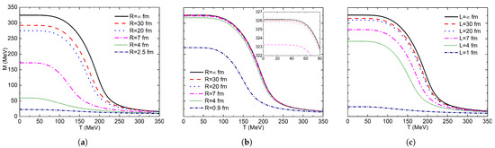
Figure 1. Constituent quark mass as a function of temperature at $\mu =0$: (a) sphere-Dirichlet; (b) sphere-Neumann; (c) cube-Dirichlet.

In cubic symmetry, these effects are considerable for a volume of 343 fm${}^3$ ($L=7$ fm), where a constituent mass of 279 MeV is obtained. A very similar mass of 275 MeV is obtained for a volume of 33,510 fm${}^3$ ($R=20$ fm) for spherical symmetry, almost a hundred times the volume of the one with spherical symmetry. Since volume effects are lower in cubic symmetry, a very small volume is needed to obtain nonconvergent results in the calculations.

The obtained results for spherical symmetry with Neumann conditions can be observed in Figure 1b, where volume effects are important for very small volumes; this is so because the surface effects disappear with these boundary conditions. These results are in agreement with the ones reported by [73]. The reduction in the mass value is negligible until $R=0.9$ fm, where constituent mass is 222 MeV. It is important to mention that the MRE scheme is not valid for very small system sizes, given that the higher order terms of the approximation were discarded. Therefore, the cubic geometry results for $R=0.9$ fm with Neumann conditions and $L=1$ fm with Dirichlet conditions must be carefully analyzed. Curvature terms are not accounted for under these two scenarios, hence the finite volume effect becomes significant for very small volumes. All obtained constituent mass values for each system are shown in Table 4.

Table 4. Constituent quark mass [MeV] for MRE systems at $\mu =0$ MeV.

	Dirichlet		Neumann
R(L) [fm]	Sphere	Cube	Sphere
∞	326.143	326.143	326.143
30	292.407	315.488	325.982
20	275.106	310.084	325.773
7	172.276	279.249	323.249
4	59.557	241.908	317.774
2.5	22.224	-	-
1	-	31.428	-
0.9	-	-	221.695

4.1.2. Finite Volume Approximation by Boundary Conditions

The behavior of constituent mass with increasing system temperature and decreasing system volume is shown in Figure 2. The order parameter is smooth for the whole interval, which implies the existence of a crossover at $\mu =0$. The APBC results in Figure 2a indicate that a very small volume is needed to observe the effects of the system size. For $L=7$ fm, the thermodynamic limit is reached; however, for $L=4$ fm, the constituent mass is 206.624 MeV, which has a negligible mass difference of 1.641 MeV compared with $L=\infty$ fm.

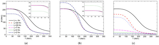
Figure 2. Constituent quark mass as a function of temperature at $\mu =0$: (a) APBC; (b) PBC; (c) SWC.

For PBC in Figure 2b, the same exact effect as APBC is shown, but in an inverse fashion: constituent mass increases with a decreasing cube size. This behavior is in agreement with the one reported by [74,75,77] in which they explain that this is because of the present fermionic zero mode. The thermodynamic limit for PBC is kept for L = 7 fm, and for $L=4$ fm, there is a very small constituent mass increase toward 210.567 MeV. Then, a very small volume is also needed to observe a significant change of the order parameter. By using SWC, Figure 2c is obtained, where a great diminishing of the constituent mass is obtained for $L=30$ fm and $M=165$ MeV, whereas for the two previous conditions, the mass value remains constant. For $L=2$ fm, the chiral symmetry restoration is practically obtained; for this size, constituent mass is $M=10$ MeV. The results for $L_{SWC}=30$ fm are approximately equal to $L_{APBC}=2$ fm. In Table 5, obtained quark constituent mass is shown for each boundary condition and sphere radius.

Table 5. Constituent quark mass [MeV] for finite volume approximation by boundary conditions at $\mu =0$ MeV.

R [fm]	APBC	PBC	SWC
∞	208.265	208.265	208.265
30	208.265	208.265	165.229
20	208.265	208.265	141.654
7	208.232	208.301	40.302
4	206.624	210.567	18.969
1	168.294	258.028	9.867

4.2. Phase Diagram

Chiral symmetry restoration occurs if the temperature and/or density is increased in such a way that the condensate disappears in the chiral limit, and at the same time, quark constituent mass is zero. In the case of finite current mass quarks, chiral condensate is not an exact order parameter because its value never reaches zero, no matter how high the temperature/density is. Nevertheless, important information of the phase diagram can be obtained from the chiral condensate through the chiral susceptibility. Chiral susceptibility ${\chi }_S$ is defined as the response of the order parameter or quark constituent mass to a perturbation of quark current mass [79,80]. The associated expression to this quantity is given by the derivative of the gap Equation (2) with respect to $m_0$

$${\chi }_S=\frac{\partial M}{\partial m_0}.$$

(21)

One of the most fundamental features of a phase diagram is the phase transition line. This line is located where the value of the order parameter presents a jump-type discontinuity [81]. An alternative way to locate this line is by means of the susceptibility related to the order parameter. This susceptibility is continuous everywhere except for the phase transition line. This discontinuity is asymptotic; however, we can only recover an intense peak by virtue of the discrete nature of our computational numerical calculations of the phase diagram. On the other hand, the susceptibility can be continuous everywhere, in which case there is no phase transition. Even if there is no phase transition, the order parameter is still bound to change value, albeit in a continuous way, rather than a discrete one. We refer to this type of change as a crossover.

Given the continuous nature of a crossover, there is no unique way to determine either its location or its width. Regarding its location, we use two different criteria with which we determine where the crossover is. The one criterion, which we call global, is based on the value of the order parameter at the global maximum of the susceptibility. This global maximum is a finite value if, and only if, there is no CEP and no first order transition curve. In case the global maximum does not exist, the criterion will be based on the value of the order parameter at the CEP instead. The other criterion, which we call local, is based on the local maxima of the susceptibility, which goes through the phase diagram. These maxima are located on a curve in the $\mu -T$ plane, and this curve’s end points are located in both axes. These maxima can also be nonfinite (asymptotic), in which case the line will go through the coordinates where these discontinuities are located. It is worth mentioning that the local criterion is the one almost universally used in the literature [79,82].

4.2.1. Multiple Reflection Expansion

In Figure 3, the phase diagrams corresponding to the local criterion are shown; the solid red dot represents the CEP, which separates the crossover region from the first-order phase transition. In the limit when $R\left(L\right)\to \infty$, the critical temperature is $T_c=206$ MeV, and the CEP is at $\mu =324$ MeV and $T=44$ MeV. For spherical geometry with Dirichlet conditions in Figure 3a, critical temperatures decrease with decreasing volume; CEP shifts quickly toward lower temperatures and slowly toward lower chemical potentials. For $R<20$ fm, the CEP disappears, and only a crossover region between both phases is obtained. The smallest computed volume is for $R=2.5$ fm, where chiral symmetry is practically restored at $T_c=9$ MeV. With the same geometry, but with Neumann conditions, the diagrams in Figure 3b were obtained; it is observed that the volume effect is negligible until $R=4$ fm, where temperature has decreased from $T_c=206$ MeV at $R\to \infty$ to only $T_c=202$ MeV. Hence, CEP coordinates are almost the same. With this boundary condition, volume effects are minimal because there is not a surface term in the density of states. For $R=0.9$ fm, the CEP disappears; hence, the line represents the crossover region. These two results are quite similar to the ones reported by [73] at the chiral limit; they reported that the temperature and chemical potential of the tri-critical point reduce as R decreases. At $R=12$ fm, the tri-critical point disappears, and the first order region vanishes. For Neumann conditions, they report that the critical temperature decreases considerably only when the size goes below $R=2$ fm, and the tri-critical point disappears when $R=1.2$ fm.

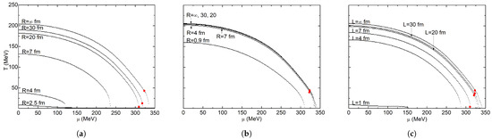
Figure 3. Phase diagram superposition for local criterion: (a) sphere-Dirichlet; (b) sphere-Neumann; (c) cube-Dirichlet. The red dots indicate the location of the CEP.

Geometry effects in the system may be observed in Figure 3c, where a significant critical temperature decrease exists until $T_c=184$ MeV for $L=7$ fm, from which the CEP disappears for lower lengths. An almost complete chiral symmetry restoration is obtained for $L=1$ fm, where $T_c=10$ MeV. The CEP trajectory presents a similar behavior to the one obtained with Dirichlet conditions and a spherical geometry. Nevertheless, the movement of the CEP through the $\mu -T$ plane was much lower in magnitude, quite like with Neumann conditions. This happens because of the lack of a curvature term contribution. Of these three schemes, the one that favors the chiral symmetry restoration the least is the spherical geometry with Neumann conditions. Even when the radius R is lower than the corresponding length on the other two schemes, chiral symmetry restoration is nowhere near as generalized. In Table 6, the trajectory of the $\mu -T$ coordinates of the CEP are shown for each boundary condition scheme. In Table 7, critical temperatures for both criterion diagrams are shown.

Table 6. Critical end point for MRE systems. $\mu$ and T are in [MeV].

	Dirichlet				Neumann
	Sphere		Cube		Sphere
R(L) [fm]	$\mathbf{\mu }$	$\mathit{T}$	$\mathbf{\mu }$	$\mathit{T}$	$\mathbf{\mu }$	$\mathit{T}$
30	318	13	322	37	324	44
20	309	1	321	33	324	44
7	-	-	311	5	324	44
4	-	-	-	-	323	40

Table 7. Phase diagram critical temperature [MeV] for MRE systems.

	Dirichlet				Neumann
	Sphere		Cube		Sphere
R(L) [fm]	loc	glob	loc	glob	loc	glob
∞	206	187	206	187	206	187
30	190	166	201	176	206	182
20	182	152	198	170	205	182
7	132	119	184	153	204	181
4	38	53	166	144	202	175
2.5	9	30	-	-	-	-
1	-	-	10	34	-	-
0.9	-	-	-	-	160	139

With the PNJL model, by using the same MRE approach, ref. [64] reports that as the system size decreases, the CEP moves toward lower temperatures, but the chemical potential remains practically constant, $\mu \simeq 312$. For the smallest system size they used ($R=2.5$), they reported a CEP at the coordinates $T=30$ MeV and $\mu =312$ MeV. With Dyson–Schwinger equations (DSEs), the infinite sum is replaced by an integration over a continuous momentum interval with a lower cutoff and neglected surface and curvature effects. The author of [83] reports that the critical and CEP temperatures decrease as the system size becomes smaller, but the CEP chemical potential increases. The CEP moves from $\mu \approx 230$ MeV and $T=103$ MeV at $R=\infty$ to $\mu \approx 355$ MeV and $T\approx 25$ MeV at $R=2.1$ fm. A similar scheme is used in the Polyakov–Quark–Meson model, where [45] introduces finite volume effects via a lower cutoff. He reports that the crossover temperature increases by $19\%$ and the chemical potential by $30\%$ as volume decreases.

The obtained phase diagrams for the global criterion are shown in Figure 4 for $R\left(L\right)\to \infty$, $T_c=187$ MeV. Local and global criteria match at the CEP, and at the first-order transition region, the CEP is located at $\mu =324$ MeV and $T=44$ MeV. The same volume effect over the phase diagrams is obtained; as system size decreases, critical temperatures decrease, and the region corresponding to the broken chiral symmetry phase shrinks.

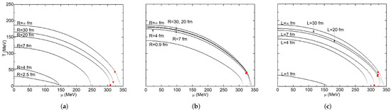
Figure 4. Phase diagram superposition for global criterion: (a) sphere-Dirichlet; (b) sphere-Neumann; (c) cube-Dirichlet. The red dots indicate the location of the CEP.

For a system with infinite volume, critical temperatures calculated with the local criterion are always higher than the ones calculated with the global criterion [84,85], but with Dirichlet conditions systems with very small volumes, the opposite happens: local criterion critical temperatures are lower than global criterion ones. This feature can be observed by comparing the phase diagrams for $L=4$ fm in Figure 3a and Figure 4a: for the local criterion $T_c=38$ MeV and for the global criterion $T_c=53$ MeV. For $L=2.5$ fm in the local criterion, chiral symmetry is almost restored at $T_c=9$ MeV, while this happens in the global criterion at $T_c=30$ MeV.

A very similar result was obtained for $L=1$ fm (Figure 3c and Figure 4c). For spherical symmetry with Neumann conditions (Figure 4b). Volume effects are significant for the global criterion at $L=4$ fm. Critical temperature decreases from $T_c=187$ MeV at $L\to \infty$ to $T_c=175$ MeV, while the local criterion decreases from $T_c=206$ MeV at $L\to \infty$, to $T_c=202$ MeV. In general, phase diagrams obtained with the global criterion are more sensitive to the system size changes. This can be inferred by the fact that the phase diagrams constructed by the local criterion are almost superimposed, while the phase diagrams constructed by the global criterion are more easily distinguishable.

4.2.2. Finite Volume Approximation by Boundary Conditions

In Figure 5, the obtained local criterion diagrams are shown. There is no CEP for $L\to \infty$, so the complete line represents a crossover, which separates the chirally broken and chirally restored phases. This agrees with [33], where a CEP appears for large bare quark masses of around 15 MeV.

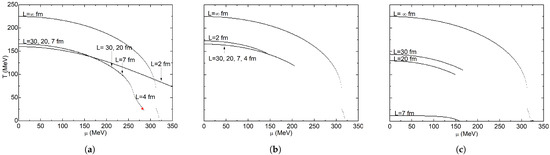
Figure 5. Phase diagram superposition for local criterion: (a) APBC; (b) PBC; (c) SWC. The red dot indicates the location of the CEP.

The finite sizes used in this work lead to considerably lower critical temperature values compared to the ones with infinite volume. Phase diagrams in Figure 5a correspond to APBC, where $T_c=166$ MeV is constant for $L=30,20,7$ and 4 fm. However, for $L=30$ and 20 fm, our calculations converged until around $\mu =210$ MeV. Introducing a finite volume to the calculations leads to unavoidable computation problems because of the lack of convergence of the gap Equation (2) at the zone of the phase diagram where the temperature is low and the chemical potential is high. As volume decreases, this chemical potential convergence limit increases. As a result, our phase diagrams reach higher chemical potential values. At $L=2$ fm, critical temperature diminishes slightly by 6 MeV compared with higher finite volumes. The lines shown in the figure represent the crossover zone, but for $L=4$ fm a CEP exists. This particular result is described in more detail in Figure 7. These results generally agree with the ones reported by [86], where DSEs are used to study a cubic box with antiperiodic boundary conditions. They report that the pseudocritical line stretches toward larger $\mu$ values and smaller T values as system size decreases. Similarly, CEP coordinates move toward higher $\mu$ values and lower temperature values: from $\mu =135$ MeV and $T=127$ MeV at $L=\infty$, to $\mu \approx 270$ MeV and $T\approx 80$ MeV at $L=2.3$ fm. They found that critical temperatures remain nearly constant for larger volumes. They did not continue with the construction of the phase diagram for temperatures smaller than 60 MeV due to computational complications derived from the Matsubara frequencies.

PBC effects are displayed in Figure 5b. As in APBC, volume effects over the critical temperature are negligible, practically remaining constant for $L=30,20,7$ and 4 fm, where $T_c=166$ MeV. Given that periodic boundary conditions imply a constituent mass increase (chiral catalysis), the critical temperature also increases. For $L=2$ fm, $T_c=173$ MeV is obtained. The presence of the zero-momentum is of crucial importance for chiral symmetry restoration. This contribution is heavily suppressed by the term ${\theta }_2(0,e^{-4{\pi }^2\tau T^2})$ only for very high temperatures, and then the chiral symmetry is restored. At low temperatures, constituent quark masses must approach $-\infty$ to solve the gap equation, and chiral symmetry restoration cannot be achieved with that unphysical constituent quark mass value [77]. This agrees with our obtained results where we could delimit the crossover zone that divides the broken and restored chiral symmetry phases at high temperatures.

In the Linear Sigma Model coupled to quarks, ref. [87] studied the finite volume effects with PBC and APBC. They found that as system size decreases, the CEP quickly moves toward very high chemical potential values and low temperature values: from $\mu \approx 210$ MeV and $T\approx 98$ MeV to $\mu \approx 558$ MeV and $T\approx 42$ MeV for PBC; and to $\mu \approx 438$ MeV and $T\approx 50$ MeV for APBC. In addition, the crossover temperature rises as the system size decreases. This effect is more notable for PBC, where temperature increases $\sim 80\%$ for $\mu =0$ and $L=2$ fm. By working with the Quark–Meson model formalism, ref. [88] found that the CEP moves toward lower temperatures and higher chemical potentials as the volume decreases: from $\mu \approx 299$ MeV and $T\approx 35$ MeV at $L=\infty$ to $\mu \approx 336$ MeV and $T\approx 9$ MeV at $L=\infty$. They found a similar behavior with APBC and PBC.

SWC results are shown in Figure 5c, where a considerable decrease in critical temperature may be observed: from $T_c=225$ MeV for $L=\infty$ fm to $T_c=144$ MeV for $L=30$ fm. For volumes smaller than $L=7$ fm, a very small chirally broken phase is enclosed at $T_c=12$ MeV. For $L=4$ and 2 fm, an extremely small chirally broken phase was found, but it was not possible to enclose by using the local criterion. All critical temperature values for local and global criteria and the maximum reached chemical potential ${\mu }_{max}$ for each cubic system size are displayed in Table 8.

Table 8. Critical temperatures [MeV] and maximun reached chemical potential [MeV] for finite volume approximation by boundary conditions systems.

	APBC			PBC			SWC
L [fm]	loc	glob	${\mathbf{\mu }}_{\mathit{max}}$	loc	glob	${\mathbf{\mu }}_{\mathit{max}}$	loc	glob	${\mathbf{\mu }}_{\mathit{max}}$
∞	225	208	320	225	208	320	225	208	320
30	166	164	210	166	163	205	144	142	166
20	166	164	213	166	163	205	130	128	149
7	166	98	242	166	164	204	12	62	158
4	166	142	285	166	165	191	-	75	269
2	160	157	547	173	169	169	-	-	350

In Figure 6, phase diagrams obtained with the global criterion are shown. It is important to note that the maximum calculated susceptibility is used as a basis in this criterion. As a result, in these built diagrams the susceptibility that was used is limited in the zone where the calculations were able to be performed, which probably is not the maximum one because the crossover zone spans the whole range of obtained values. For $R\to \infty$ fm, we obtained a $T_c=208$ MeV, quite unlike the local criterion. A greater effect of the system size decrease over the crossover critical temperatures is observed for the global criterion. In general, a volume decrease leads to a critical temperature value decrease; however, for very small volumes, such as $L=4$ and 2 fm, critical temperature increases. Hence, the region corresponding to the broken chiral phase increases in size. Regarding Figure 6a for APBC, $T_c=164$ MeV for $L=30$ and 20 fm, this value is nearly equal to the one of the local criterion, but for $L=7$ fm, the critical temperature decreases to $T_c=98$ MeV. In this size, phases are almost totally delimited by the crossover. The same behavior from the local criterion is obtained for the diagrams in Figure 6b for PBC; the volume effect in these conditions is negligible. Critical temperature stays around $T_c=163$ MeV and slightly increases for $L=2$ fm to $T_c=169$ MeV.

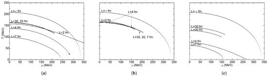
Figure 6. Phase diagram superposition for global criterion: (a) APBC; (b) PBC; (c) SWC. The red dot indicates the location of the CEP.

In fact, critical temperatures for all finite volumes are practically the same for the local and global criteria. The diagrams in Figure 6c were obtained with the SWC; critical temperature decreases from $T_c=208$ MeV at $L=\infty$ to $T_c=142$ MeV at $L=30$ MeV. Unlike the local criterion, at $L=7$ fm a larger chirally restored phase is obtained; the size of this phase increases when the system volume decreases to $L=4$ fm. All obtained critical temperatures in the local criterion are higher than their global criterion counterparts, except for the SWC system at $L=7$ fm, where the global criterion critical temperature is much higher than the local criterion one.

In Figure 7, phase diagrams for APBC are shown; with very small volumes, the presence of a CEP and a first order phase transition is favored. As the volume decreases, the CEP moves toward higher chemical potentials.

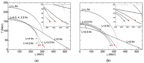
Figure 7. APBC phase diagram superposition for small volumes: (a) local criterion; (b) global criterion. The red dots indicate the location of the CEP.

For $L=4.5$ fm, the CEP is located at $T=23$ MeV and $\mu =269$ MeV, but we were only able to obtain a single point beyond the CEP in the first order transition region for $\mu =270$ MeV. There is no CEP for $L>4.5$ fm. For $L=4$ fm, the CEP is located at $T=25$ MeV and $\mu =283$ MeV; a small first order transition line is also obtained. When the cube has an edge $L=3.5$ fm, the CEP is located at $T=25$ MeV and $\mu =306$ MeV; the size of the first order transition line increases its size slightly. The smallest diagram where crossover separated phases could be obtained was at $L=2$ fm; the obtained crossover region extends to very high chemical potentials and the CEP appears at $T=10$ MeV and $\mu =517$ MeV. Under these conditions, the first order transition line crosses the chemical potential axis at $\mu =547$ MeV.

A comparison of the six different schemes is shown in Figure 8. All lengths are equal to 7 fm, but it is important to mention that this length is equal to the radius R in spherical schemes, while it is equal to the edge L in cubic schemes. For both criteria, the cubic SWC scheme is the one that favors chiral symmetry restoration the most; chiral symmetry is nearly restored for the whole diagram according to the local criterion. On the other hand, the spherical Neumann condition scheme is the one that obstructs chiral symmetry restoration the most. For all cases, the chirally broken region is smaller in the global criterion compared to the local one. Moreover, we were able to obtain more diagrams that extend all the way to the chemical potential axis with the global criterion. As an example, the APBC case of the phase diagram shown in Figure 8b displays a complete crossover curve that ends at the chemical potential axis; however, its local counterpart does not (Figure 8a).

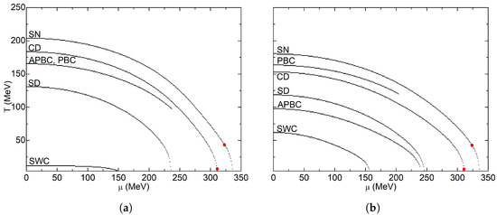
Figure 8. Phase diagram superposition for $R=L=7$ fm. SN: sphere-Neumann; CD: cube-Dirichle; SD: sphere-Dirichlet; APBC: antiperiodic boundary conditions; PBC: periodic boundary conditions; SWC: stationary wave conditions. (a) local criterion; (b) global criterion. The red dots indicate the location of the CEP.

4.3. Crossover Zone

The crossover is a region of the phase diagram where the order parameter changes value on a continuous fashion. Physically, this can be interpreted as a zone where the matter interactions resemble both phases when a phase transition is present. However, the location and width of the crossover zone is arbitrary until some point, in contrast to a phase transition in which its discontinuity can be located without ambiguity. In strict mathematical terms, the crossover zone occupies the whole phase diagram until it reaches the CEP, and the phase transition proper takes off from there. If there is no CEP present, the crossover occupies the entire diagram. However, this is not useful from a phenomenological standpoint because that does not say anything about the properties of the strongly interacting matter at different temperatures or chemical potentials.

One of the objectives of determining a definite location and a finite width of the crossover zone is to distinguish different zones of the phase diagram where the order parameter changes more quickly or more slowly, albeit always continuously. A convenient phenomenological description of the crossover takes into account only the zones where the order parameter changes quickly, but this is obviously subjective unless some limit to the rate of change of the order parameter is established (even if this limit is also subjective).

Taking advantage of the fact that for any perpendicular plane to the $\mu -T$ plane (where the susceptibility is the additional axis), the susceptibility is described by a bell-like curve. It is convenient to establish the extent of the crossover as the zone of the diagram where the susceptibility values are closest to the crest. The location of the crest is interpreted as the location of the crossover, and this is analogous to the local maximum in one variable functions. To determine which values are close to the crest and which are not, the curves where the Hessian matrix has zero determinant will act as the lower and higher limits of the crossover zone, analogous with the inflection points in one variable functions.

Given that the crests (or the vertical asymptotes) will always be contained between the two limits described by the inflection points, this way of defining the extent of the crossover will always ensure that the location of the crossover according to the local criterion is contained between these two limits, although this is not necessarily true for the global criterion. Nevertheless, both criteria will always agree with the location of the CEP and the first order phase transition line (if they exist).

The phase diagrams in Figure 9 were obtained for an infinite volume system. The proper time regularization diagram is displayed in Figure 9a, where a thick band that represents the crossover region can be observed. There is no CEP, so the band continues practically with a constant width until it reaches the chemical potential axis. When a CEP exists, such as in Figure 9b, the band reduces its width until it reaches the CEP, from which it continues as a line that represents the first order transition. This diagram corresponds to the UV cutoff regularization scheme.

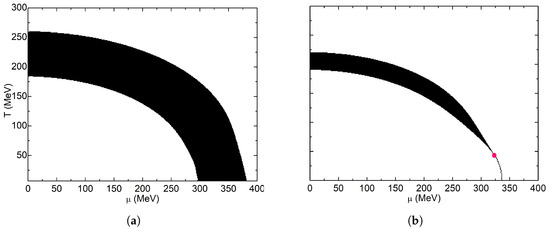
Figure 9. Inflection point criterion phase diagram for infinite volume systems: (a) proper time regularization; (b) ultraviolet cutoff. The red dot indicates the location of the CEP.

4.3.1. Multiple Reflection Expansion

For the spherically symmetric Dirichlet condition scheme, the corresponding phase diagrams can be observed in Figure 10. In these, the first order transition disappears with a decreasing system volume, the crossover width increases and the temperature range moves toward lower temperatures. For very small volumes, a very wide crossover region that extends over the whole chemical potential axis is obtained; in this state, the size of the chirally broken phase is almost insignificant.

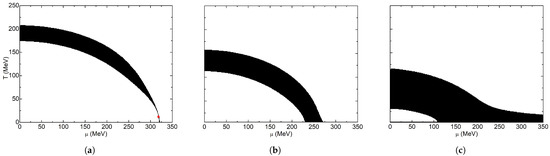
Figure 10. Inflection point criterion phase diagram for spherical geometry with Dirichlet boundary conditions: (a) R = 30 fm; (b) R = 7 fm; (c) R = 4 fm. The red dot indicates the location of the CEP.

With spherically symmetric Neumann conditions, the crossover region does not change (Figure 11). It keeps the same width, and its temperature range moves downward by a few units. In Figure 12, the cubically symmetric Dirichlet boundary condition scheme can be observed. The crossover region keeps its width, but the temperature interval moves downward. Meanwhile, the high chemical potential zone of the crossover increases its width until the CEP disappears, and the crossover region occupies the whole diagram. This behavior is similar to the one displayed in Figure 11, but the cubic symmetry of Figure 12 causes the gradual (less abrupt) crossover widening in high chemical potentials.

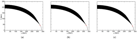
Figure 11. Inflection point criterion phase diagram for spherical geometry with Neumann boundary conditions: (a) R = 30 fm; (b) R = 7 fm; (c) R = 4 fm. The red dots indicate the location of the CEP.

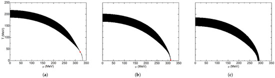
Figure 12. Inflection point criterion phase diagram for cubic geometry with Dirichlet boundary conditions: (a) R = 30 fm; (b) R = 7 fm; (c) R = 4 fm. The red dot indicates the location of the CEP.

4.3.2. Finite Volume Approximation by Boundary Conditions

With SWC, the obtained diagrams can be seen in Figure 13. For larger volumes, we obtained a constant width band that continued until we were not able to calculate the order parameter at that chemical potential value. By reducing the volume, the band width increases drastically, and the crossover zone becomes very wide, taking the majority of the displayed region of the $T-\mu$ plane for $L=4$ fm. For $L=7$ and 4 fm, a small chirally broken phase can be appreciated. For smaller volumes, a very wide band is obtained. This band stretches over the whole chemical potential range ($\mu ϵ[0,350]$ MeV). In Figure 14, the evolution of the extension of the first order transition line can be observed. The sharp part of the diagram at the end of the crossover region is lengthening as the volume decreases. In addition, the crossover width and range for low chemical potentials remains constant, which agrees with the diagrams seen in Figure 7. For lesser volumes ($L=1$ fm), a very wide crossover zone is obtained, such as in SWC. This zone occupies the whole temperature and chemical potential intervals used in this work. The obtained phase diagrams with this criterion for PBC were very similar to the one seen in Figure 13a for all finite values for L.

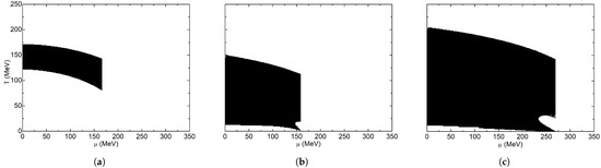
Figure 13. Inflection point criterion phase diagram for stationary wave conditions: (a) L = 30 fm; (b) L = 7 fm; (c) L = 4 fm.

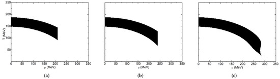
Figure 14. Inflection point criterion phase diagram for anti-periodic boundary conditions: (a) L = 30 fm; (b) L = 7 fm. (c) L = 4 fm.

In general, we found out that the crossover behavior in a boundary condition scheme follows a few trends. One of them is that the width of the crossover band invariably becomes wider. This is more obvious for SWC, but it also happens in APBC. Another curious thing is that we are able to obtain higher chemical potentials of the phase diagram for smaller volumes. For APBC we were even able to retrieve the CEP at $L=4$ fm.

5. Summary and Conclusions

In this work, the effect of the finite volume on the chiral phase transition was studied in the framework of the two-flavor Nambu–Jona–Lasinio model at finite temperature and chemical potential with the mean field approximation. One of the two ways we introduced a finite system size was with a multiple reflection expansion, where both an infrared and ultraviolet cutoff on the three-momentum regularize the integrals, and finite volume effects are introduced via a modification of the density of states. Under Dirichlet conditions for a spherical geometry, the broken chiral symmetry phase occupies a lesser region in the $\mu -T$ plane as the volume shrinks. Moreover, the CEP that appears in the thermodynamic limit moves toward lower temperature and chemical potential values until it disappears for $R<20$ fm. On the other hand, cubic geometry has a lesser effect on the phase diagram. We obtained an important qualitative change when $L\le 7$ fm. It is from this size toward lower sizes where the CEP disappears. Regarding the Neumann conditions, system size does have a negligible effect on the phase diagram. The width of the crossover zone remained the same throughout all system sizes, and the CEP and the first order transition remained at the same set of $\mu -T$ coordinates. Generally, in the MRE formalism, the CEP shifts toward lower temperature values and remains almost constant in its chemical potential value.

Another way with which we studied the finite volume effects was by using a proper time regularization to control divergences. After that, the three-momentum integration was replaced by a sum over discrete momentum modes that depends on the specific applied boundary condition: APBC, PBC or SWC. In the thermodynamic limit, we obtained a crossover zone whose width remains almost the same throughout the whole $\mu -T$ plane. As a result, we did not find a CEP. We found that the antiperiodic boundary conditions support the chiral symmetry restoration, the existence of a CEP and the existence of a small but growing first order phase transition line. As the cube size shrinks, the first order transition line grows in size, and the CEP moves toward higher chemical potential values and lower temperature values. Stationary wave conditions favor chiral symmetry restoration for the smallest volumes (where a small broken chiral symmetry phase was able to be delimited). However, unlike with APBC, the crossover zone is much wider, and as the cube size shrinks, the width increases until it occupies the whole calculated region of the $\mu -T$ plane. In a completely opposite way to the other two boundary conditions, PBC favors the spontaneous chiral symmetry breaking. We were able to delimit the crossover zone only for high temperatures and low chemical potentials. Moreover, as the length of the edge of the cube decreases, the system remains virtually with no changes. All of this is because of the zero mode that causes an increase in quark condensation, preventing chiral symmetry restoration. For the smallest sizes in all system configurations, we obtained a widespread crossover zone that filled the whole interval that separates the broken symmetry phase and the restored symmetry phase.

One particular curiosity about the proper time regularization boundary condition schemes was the computational difficulties that we came across at high chemical potentials. We were able to obtain a complete APBC phase diagram only at $L=4$ fm, in which we recovered a CEP, and we were never able to obtain a single complete phase diagram for SWC. We believe this issue is not physical, but rather computational: the convergence area for iterative numerical methods is likely becoming smaller as the chemical potential increases, and this convergence area can become even smaller than the tolerance commonly used in these computer algorithms.

In conclusion, theoretical approaches to the QCD phase diagram through effective theories such as the NJL model can be of great utility. Many experimental efforts are currently being made to know more about the QCD phase diagram, but in the low chemical potential zone most of them are already able to achieve, we know, up to a certain degree of accuracy, that the corresponding zone of the phase diagram to the one currently experimentally achievable is the crossover. This is why it is so important to be able to determine its characteristics, such as its location or its width. We believe that being able to qualitatively describe the crossover is fundamental because many experiments have already gotten there. With the firsthand measurements achieved in all those experimental efforts, this zone of the QCD phase diagram is likely the first we will fully understand.

Appendix A.1. Spherical Droplet Shape

The volumetric density of states, which is the number of states per unit interval of momentum, is given by

$$\begin{array}{c}\hfill \mathrm{d}{N}_{vol}={\displaystyle \frac{V}{{(2\pi )}^3}}{\mathrm{d}}^3\mathit{p},\end{array}$$

(A1)

in spherical coordinates, the term ${\mathrm{d}}^3\mathit{p}$ becomes $4\pi p^2\mathrm{d}p$ which allows us to write the density of states in the form

$$\begin{array}{c}\hfill \rho \left(p\right)={\displaystyle \frac{\mathrm{d}{N}_{vol}}{\mathrm{d}p}}=V{\displaystyle \frac{p^2}{2{\pi }^2}},\end{array}$$

(A2)

This definition can be extended to the framework of multiple reflection expansion (MRE) [62,63,64] that leads to a liquid drop model which means that it is possible to study a sphere of radius R that encloses a quark matter system. The density of states per unit volume in the (MRE) for a sphere is given by [65,66]

$${\rho }_{MRE}={\displaystyle \frac{p^2}{2{\pi }^2}}\left[1+{\displaystyle \frac{6{\pi }^2}{pR}}{f}_S\left(\frac{p}{\alpha }\right)+{\displaystyle \frac{12{\pi }^2}{{\left(pR\right)}^2}}{f}_C\left(\frac{p}{\alpha }\right)\right],$$

(A3)

where

$$\begin{array}{cc}\hfill f_S\left(\frac{p}{\alpha }\right)& \hfill =-\frac{1}{8\pi }\left[1-\frac{2}{\pi }arctan\frac{p}{\alpha }\right],\hfill \end{array}$$

(A4)

$$\begin{array}{cc}\hfill f_C\left(\frac{p}{\alpha }\right)& \hfill =\frac{1}{12{\pi }^2}\left[1-\frac{3p}{2\alpha }\left(\frac{\pi }{2}-arctan\frac{p}{\alpha }\right)\right],\hfill \end{array}$$

(A5)

are the the surface and curvature contributions to the density of states, respectively. The parameter $\alpha$ is related to the penetration of the wave function of the quark matter confined in a finite volume into the hadronic medium [67].

Equation (A3) being a quadratic one, it may happen that there is an interval of p values in which the density of states takes negative values which are physically not allowed. To avoid this problem, an infrared (IR) cutoff is defined for the value of the momentum p in the lower limit of integration of (2). The following replacement is performed [64]

$$\int \frac{{\mathrm{d}}^3\mathit{p}}{{(2\pi )}^3}f(T,\mu ,\mathit{p})\to {\int }_0^{\infty }\mathrm{d}p\rho \left(p\right)f(T,\mu ,p)\to {\int }_{{\Lambda }_{IR}}^{{\Lambda }_{UV}}\mathrm{d}p{\rho }_{MRE}(p,\alpha ,R)f(T,\mu ,p),$$

(A6)

where ${\Lambda }_{IR}$ is the largest solution to ${\rho }_{MRE}(p,\alpha ,R)=0$ with respect to momentum p. The momentum integrals are limited in the upper limit by ${\mathit{p}}^2={\Lambda }_{UV}^2$ [71], where ${\Lambda }_{UV}$ is the three-momentum cutoff. Following [72,73], a Dirichlet boundary condition is imposed by setting $\alpha =\infty$ in (A4) and (A5) to obtain

$$\begin{array}{cc}\hfill \underset{\alpha \to \infty }{lim}{f}_S\left(\frac{p}{\alpha }\right)& \hfill =-\frac{1}{8\pi },\hfill \end{array}$$

(A7)

$$\begin{array}{cc}\hfill \underset{\alpha \to \infty }{lim}{f}_C\left(\frac{p}{\alpha }\right)& \hfill =\frac{1}{12{\pi }^2},\hfill \end{array}$$

(A8)

and the infrared cutoff is written as

$$\begin{array}{c}\hfill {\Lambda }_{IR}={\displaystyle \frac{1.8}{R}},\end{array}$$

(A9)

once boundary conditions (A7) and (A8) are established, the density of states (Equation (A3)) takes the form:

$$\begin{array}{c}\hfill {\rho }_{MRE}={\displaystyle \frac{p^2}{2{\pi }^2}}\left[1-{\displaystyle \frac{3\pi }{4pR}}+{\displaystyle \frac{1}{{\left(pR\right)}^2}}\right].\end{array}$$

(A10)

On the other hand, to be consistent with the MIT Bag model, the Neumann boundary conditions are applied for $\alpha =0$ [72]

$$\begin{array}{cc}\hfill \underset{\alpha \to 0}{lim}{f}_S\left({\displaystyle \frac{k}{\alpha }}\right)& \hfill =0,\hfill \end{array}$$

(A11)

$$\begin{array}{cc}\hfill \underset{\alpha \to 0}{lim}{f}_C\left({\displaystyle \frac{k}{\alpha }}\right)& \hfill =-{\displaystyle \frac{1}{24{\pi }^2}},\hfill \end{array}$$

(A12)

and the infrared cutoff is

$$\begin{array}{c}\hfill {\Lambda }_{IR}={\displaystyle \frac{1}{\sqrt{2}R}}.\end{array}$$

(A13)

Appendix A.2. Cubic Box

For a sphere, in the MRE model there are three terms in the expression for density of states (A3). The first term is the volumetric density, the second is the surface density, and the last refers to the curvature, this is

$${\rho }_{MRE}={\rho }_{vol}+{\rho }_{surf}+{\rho }_{curv},$$

(A14)

where in the case of a cubic geometry, ${\rho }_{vol}$ is defined in the same fashion as the sphere in Equation (A1). In analogy to volumetric density in Equation (A1), we can define a surface density of states for ${\rho }_{Asurf}$

$$\begin{array}{c}\hfill \mathrm{d}{N}_{surf}={\displaystyle \frac{A}{{(2\pi )}^2}}{\mathrm{d}}^2\mathit{p},\end{array}$$

(A15)

where $A=6L^2$ represents the area of the six sides of a cube, and in polar coordinates, we have ${\mathrm{d}}^2\mathit{p}=2\pi p\mathrm{d}p$. Then the surface density of states as a function of volume, $V={\displaystyle \frac{AL}{6}}$ is

$$\begin{array}{c}\hfill {\displaystyle \frac{\mathrm{d}{N}_{surf}}{\mathrm{d}p}}={\displaystyle \frac{Vp}{2\pi L}},\end{array}$$

(A16)

the curvature contribution $f_{curv}$ is zero due to the fact that we are working inside a cubic shape, thus ${\rho }_{curv}=0$. Therefore, the density of states per unit volume for a cubic system in the MRE model reads

$$\begin{array}{c}\hfill {\rho }_{MRE}={\displaystyle \frac{k^2}{2{\pi }^2}}\left(1-{\displaystyle \frac{3}{4kL}}\right).\end{array}$$

(A17)

Just as it was already described for a spherical volume, there are two roots of the density of states (A17) in the p axis, and the density is negative between these zeroes. To avoid this unphysical feature of the model, the interval between $p=0$ and $p=3/4L$ is not taken into account, and the higher root is taken as an infrared cutoff ${\Lambda }_{IR}$

$${\Lambda }_{IR}=\frac{0.75}{L}.$$

(A18)

Appendix B.1. Periodic Boundary Conditions PBC

Here, it is assumed for quark fields $q(\mathit{x}=0)=q(\mathit{x}=L)$, and the reachable momentum modes values are given by $p_n=2n\pi /L$ for $n=0,\pm 1,\pm 2,\dots$. Therefore, for all n values we have

$$\begin{array}{c}\hfill \sum _n{p}_n^2={\displaystyle \frac{4{\pi }^2}{L^2}}\sum _{n=-\infty }^{\infty }{n}^2,\end{array}$$

(A25)

then, for the three-momentum, we define $n^2=n_x^2+n_y^2+n_z^2$, replacing (17) and (A25) in (A24)

$$\begin{array}{c}\hfill \int {\displaystyle \frac{{\mathrm{d}}^3\mathit{p}}{{(2\pi )}^3}}{e}^{-\tau {\mathit{p}}^2}={\displaystyle \frac{1}{L^3}}{\left[\sum _n^{\infty }exp\left(\frac{-4{\pi }^2\tau }{L^2}{n}^2\right)\right]}^3,\end{array}$$

(A26)

let $q\equiv e^{-4{\pi }^2\tau /L^2}$, therefore ${\Theta }_3\left[0,q\right]\equiv {\sum }_n{q}^{n^2}$. Finally the chiral quark condensate for a finite volume with PBC reads

$$\begin{array}{c}\hfill ⟨\overline{q}qi⟩=-4M{N}_c{N}_{f}T{\int }_{{\tau }_{UV}}^{\infty }\mathrm{d}\tau e^{-\tau (M^2-{\mu }^2)}\hfill \\ \hfill \times {\Theta }_2\left[-2\tau \pi T\mu ,e^{-4{\pi }^2{T}^2\tau }\right]{\displaystyle \frac{1}{L^3}}{\left\{{\Theta }_3\left[0,e^{-4{\pi }^2\tau /L^2}\right]\right\}}^3.\end{array}$$

(A27)

Appendix B.2. Antiperiodic Boundary Conditions APBC

Under APBC, we define $q(\mathit{x}=0)=-q(\mathit{x}=L)$, and the momentum values are $p=(2n+1)\pi /L$ for $n=0,\pm 1,\pm 2,\dots$, then the whole momentum spectrum is

$$\begin{array}{c}\hfill \sum _n{p}_n^2={\displaystyle \frac{4{\pi }^2}{L^2}}\sum _{n=-\infty }^{\infty }{\left(n+\frac{1}{2}\right)}^2,\end{array}$$

(A28)

thus

$$\begin{array}{c}\hfill \int {\displaystyle \frac{{\mathrm{d}}^3\mathit{p}}{{(2\pi )}^3}}{e}^{-\tau {\mathit{p}}^2}={\displaystyle \frac{1}{L^3}}{\left[\sum _n^{\infty }{e}^{\left(-\frac{4{\pi }^2\tau }{L^2}\right){\left(n+\frac{1}{2}\right)}^2}\right]}^3,\end{array}$$

(A29)

let $q=e^{-4{\pi }^2\tau /L^2}$, in this case for $(n+1/2)$ we introduce the Jacobi ${\Theta }_2$-function

$$\begin{array}{c}\hfill ⟨\overline{q}q⟩=-4M{N}_c{N}_{f}T{\int }_{{\tau }_{UV}}^{\infty }\mathrm{d}\tau e^{-\tau (M^2-{\mu }^2)}\hfill \\ \hfill \times {\Theta }_2\left[-2\tau \pi T\mu ,e^{-4{\pi }^2{T}^2\tau }\right]{\displaystyle \frac{1}{L^3}}{\left\{{\Theta }_2\left[0,e^{-4{\pi }^2\tau /L^2}\right]\right\}}^3.\end{array}$$

(A30)

With this redefinition of momentum given by (A25) and (A28) at finite volume, the discretized momentum p is established in terms of n, its maximum value corresponds to the UV-cutoff ${\Lambda }_{UV}$

$$\begin{array}{c}\hfill p_{max}={\Lambda }_{UV}={\displaystyle \frac{2n_{max}\pi }{L}},\end{array}$$

(A31)

for the minimum value we have $n_{min}=1$.

Appendix B.3. Stationary Wave Conditions SWC

In the case, the function takes zero value at both ends. This is equivalent to having a field enclosed inside a box with finite volume $q(\mathit{x}=0)=q(\mathit{x}=L)=0$. Then the momentum is $p=n\pi /L$, for $n=1,2,\dots$, the summation for all momentum is

$$\begin{array}{c}\hfill \sum _n{p}_n^2={\displaystyle \frac{{\pi }^2}{L^2}}\sum _{n=0}^{\infty }{n}^2,\end{array}$$

(A32)

and

$$\begin{array}{c}\hfill \int {\displaystyle \frac{{\mathrm{d}}^3\mathit{p}}{{(2\pi )}^3}}{e}^{-\tau {\mathit{p}}^2}={\displaystyle \frac{1}{L^3}}{\left[\sum _{n=0}^{\infty }{e}^{(-{\pi }^2\tau /L^2)n^2}\right]}^3,\end{array}$$

let $q\equiv e^{-{\pi }^2\tau /L^2}$, then we have ${\Theta }_3\left[0,q\right]=1+{\sum }_{n=1}^{\infty }{q}^{n^2}$, after that the gap Equation (A24) for a finite volume with SWC can be written as

$$\begin{array}{c}\hfill ⟨\overline{q}q⟩=-4M{N}_c{N}_{f}T{\int }_{{\tau }_{UV}}^{\infty }\mathrm{d}\tau e^{-\tau (M^2-{\mu }^2)}{\Theta }_2\left[-2\tau \pi T\mu ,e^{-4{\pi }^2{T}^2\tau }\right]\hfill \\ \hfill \times {\displaystyle \frac{1}{8L^3}}{\left\{{\Theta }_3\left[0,e^{-{\pi }^2\tau /L^2}\right]-1\right\}}^3.\end{array}$$

(A33)

References

- Goldstone, J. Field theories with ≪Superconductor≫ solutions. Nuovo Cim. 1961, 19, 154–164. [Google Scholar] [CrossRef]
- Weise, W. QCD aspects of hadron physics. Nucl. Phys. A 2000, 670, 1–4. [Google Scholar] [CrossRef]
- Sharma, S. Updates on the QCD phase diagram from lattice. AAPPS Bull. 2021, 31, 13. [Google Scholar] [CrossRef]
- Wang, P. Color confinement, dark matter and the missing anti-matter. J. Phys. G Nucl. Part. Phys. 2021, 48, 105002. [Google Scholar] [CrossRef]
- Guenther, J.N. Overview of the QCD phase diagram. Eur. Phys. J. A 2021, 57, 136. [Google Scholar] [CrossRef]
- Philipsen, O. The QCD equation of state from the lattice. Prog. Part. Nucl. Phys. 2013, 70, 55–107. [Google Scholar] [CrossRef]
- Ding, H.-T.; Karsch, F.; Mukherjee, S. Thermodynamics of strong-interaction matter from lattice QCD. Int. J. Mod. Phys. E 2015, 24, 1530007. [Google Scholar] [CrossRef]
- Fukushima, K.; Hatsuda, T. The phase diagram of dense QCD. Rep. Prog. Phys. 2011, 74, 014001. [Google Scholar] [CrossRef]
- Cuteri, F.; Philipsen, O.; Sciarra, A. On the order of the QCD chiral phase transition for different numbers of quark flavours. J. High Energy Phys. 2021, 2021, 141. [Google Scholar] [CrossRef]
- Tomboulis, E.T. Chiral symmetry restoration at large chemical potential in strongly coupled SU(N) gauge theories. J. Math. Phys. 2013, 54, 122301. [Google Scholar] [CrossRef]
- Skullerud, J.-I.; Hands, S.; Kim, S. The onset and deconfinement transitions in two-colour QCD. arXiv 2005, arXiv:hep-lat/0511001. [Google Scholar]
- Ipek, S.; Tait, T.M.P. Early cosmological period of QCD confinement. Phys. Rev. Lett. 2019, 122, 112001. [Google Scholar] [CrossRef] [PubMed]
- Scharenberg, R.P.; Srivastava, B.K.; Hirsch, A.S.; Pajares, C. Hot dense matter: Deconfinement and clustering of color sources in nuclear collisions. Universe 2018, 4, 96. [Google Scholar] [CrossRef]
- Busza, W.; Rajagopal, K.; van der Schee, W. Heavy Ion Collisions: The big picture, and the big questions. Ann. Rev. Nucl. Part. Sci. 2018, 68, 339–376. [Google Scholar] [CrossRef]
- Dolgov, A.D.; Pozdnyakov, N.A. Asymmetric baryon capture by primordial black holes and baryon asymmetry of the Universe. Phys. Rev. D 2021, 104, 083524. [Google Scholar] [CrossRef]
- Elahi, F.; Meharabpour, H. Magnetogenesis from baryon asymmetry during an early matter dominated era. Phys. Rev. D 2021, 104, 115030. [Google Scholar] [CrossRef]
- Dvornikov, M.; Semikoz, V.B. Influence of the hypermagnetic field noise on the baryon asymmetry generation in the symmetric phase of the early universe. Eur. Phys. J. C 2021, 81, 1001. [Google Scholar] [CrossRef]
- Chaudhuri, A.; Khlopov, M.Y. Balancing asymmetric dark matter with baryon asymmetry and dilution of frozen dark matter by sphaleron transition. Universe 2021, 7, 275. [Google Scholar] [CrossRef]
- Xu, S.-S. QCD equation of state and the structure of neutron stars in NJL model. Nucl. Phys. B 2021, 917, 115540. [Google Scholar] [CrossRef]
- Orsaria, M.; Rodrigues, H.; Weber, F.; Contrera, G.A. Quark deconfinement in high-mass neutron stars. Phys. Rev. C 2014, 89, 015806. [Google Scholar] [CrossRef]
- McLerran, L.; Reddy, S. Quarkyonic matter and neutron stars. Phys. Rev. Lett. 2019, 122, 122701. [Google Scholar] [CrossRef] [PubMed]
- Roupas, Z.; Panotopoulos, G.; Lopes, I. QCD color superconductivity in compact stars: Color-flavor locked quark star candidate for the gravitational-wave signal GW190814. Phys. Rev. D 2021, 103, 083015. [Google Scholar] [CrossRef]
- Baldo, M.; Burgio, G.F.; Castorina, P.; Plumari, S.; Zappalá, D. Quark matter in neutron stars within the Nambu-Jona-Lasinio model and confinement. Phys. Rev. C 2007, 75, 035804. [Google Scholar] [CrossRef]
- Stephanov, M.A. QCD phase diagram and the critical point. Int. J. Mod. Phys. A 2005, 20, 4387–4392. [Google Scholar] [CrossRef]
- Ayala, A.; Bashir, A.; Cobos-Martínez, J.J.; Hernández-Ortiz, S.; Raya, A. The effective QCD Phase diagram and the critical end point. Nucl. Phys. B 2015, 897, 77–86. [Google Scholar] [CrossRef][Green Version]
- Bernhardt, J.; Fischer, C.S.; Isserstedt, P.; Schaefer, B.-J. Critical endpoint of QCD in a finite volume. Phys. Rev. D 2021, 104, 074035. [Google Scholar] [CrossRef]
- Pásztor, A.; Borsanyi, S.; Fodor, Z.; Kapas, K.; Katz, S.D.; Giordano, M.; Nogradi, D.; Wong, C.H. New approach to lattice QCD at finite density: Reweighting without an overlap problem. arXiv 2021, arXiv:2112.02134v2. [Google Scholar]
- Mondal, S.; Mukherjee, S.; Hedge, P. Lattice QCD equation of state for nonvanishing chemical potential by resumming Taylor expansions. Phys. Rev. Lett. 2022, 128, 022001. [Google Scholar] [CrossRef]
- Liu, L.-M.; Xu, J.; Peng, G.-X. Three-dimensional QCD phase diagram with pion condensate in the NJL model. Phys. Rev. D 2021, 104, 076009. [Google Scholar] [CrossRef]
- Aoki, Y.; Endr Hodi, G.; Fodor, Z.; Katz, S.; Szabo, K. The order of quantum chromodynamics transition predicted by the standard model of particle physics. Nature 2006, 443, 675–678. [Google Scholar] [CrossRef]
- Bazavov, A.; Ding, H.-T.; Hegde, P.; Kaczmarek, O.; Karsch, F.; Karthik, N.; Laermann, E.; Lahiri, A.; Larsen, R.; Li, S.-T.; et al. Chiral crossover in QCD at zero and non-zero chemical potentials. Phys. Lett. B 2019, 795, 15–21. [Google Scholar] [CrossRef]
- Borzányi, S.; Fodor, Z.; Hoelbling, C.; Katz, S.D.; Krieg, S.; Szabóae, K.K. Full result for the QCD equation of state with 2+1 flavors. Phys. Lett. B 2014, 730, 99–104. [Google Scholar] [CrossRef]
- Kohyama, H.; Kimura, D.; Inagaki, T. Regularization dependence on phase diagram in Nambu–Jona-Lasinio model. Nucl. Phys. B 2015, 896, 682–715. [Google Scholar] [CrossRef]
- ALICE Collaboration. Measurement of the cross sections of and baryons and of the branching-fraction ratio BR(→Ξ−e+νe)/BR(→Ξ−π+) in pp collisions at = 13 TeV. Phys. Rev. Lett. 2021, 127, 272001. [Google Scholar] [CrossRef]
- ALICE Collaboration. Inclusive J/ψ production at midrapidity in pp collisions at = 13 TeV. Eur. Phys. J. C 2021, 81, 1121. [Google Scholar] [CrossRef]
- STAR Collaboration. Measurement of cold nuclear matter effects for inclusive J/ψ in p+Au collisions at = 200 GeV. Phys. Lett. B 2022, 825, 136865. [Google Scholar] [CrossRef]
- Senger, P. Heavy-ion collisions at FAIR-NICA energies. Particles 2021, 4, 214–226. [Google Scholar] [CrossRef]
- Blume, C. Particle Production at the SPS and the QCD Phase Diagram. J. Phys. Conf. Ser. 2010, 230, 012003. [Google Scholar] [CrossRef]
- Gazdzicki, M.; Rybicki, A. Overview of results from NA61/SHINE: Uncovering critical structures. Acta Phys. Pol. B 2019, 50, 1057–1070. [Google Scholar] [CrossRef]
- Monnai, A.; Schenke, B.; Shen, C. QCD equation of state at finite chemical potentials for relativistic nuclear collisions. Int. J. Mod. Phys. A 2021, 36, 2130007. [Google Scholar] [CrossRef]
- Andronic, A.; Braun-Munzinger, P.; Redlich, K.; Stachel, J. Decoding the pahse structure of QCD via particle production at high energy. Nature 2018, 561, 321–330. [Google Scholar] [CrossRef] [PubMed]
- Shuryak, E. Physics of Strongly Coupled Quark-Gluon Plasma. Prog. Part. Nucl. Phys. 2009, 62, 48–101. [Google Scholar] [CrossRef]
- Abreu, L.; Correa, E.; Linhares, C.; Malbouisson, A. Finite-volume and magnetic effects on the phase structure of the three-flavor Nambu–Jona-Lasinio model. Phys. Rev. D 2019, 99, 076001. [Google Scholar] [CrossRef]
- Wang, Q.; Xia, Y.; Zong, H. Nambu–Jona-Lasinio model with proper time regularization in a finite volume. Mod. Phys. Lett. A 2018, 33, 1850232. [Google Scholar] [CrossRef]
- Magdy, N. Influence of finite volume effect on the Polyakov Quark-Meson model. Universe 2019, 5, 94. [Google Scholar] [CrossRef]
- Liu, R.-L.; Lai, M.-Y.; Shi, C.; Zong, H.-S. Finite volume effect on QCD susceptibilities with a chiral chemical potential. Phys. Rev. D 2020, 102, 014014. [Google Scholar] [CrossRef]
- Xu, Y.; Shi, C.; He, X.; Zong, H. Chiral crossover transition from the Dyson-Schwinger equations in a sphere. Phys. Rev. D 2020, 102, 114011. [Google Scholar] [CrossRef]
- Zhang, Z.; Shi, C.; Zong, H. Nambu-Jona-Lasinio model in a sphere. Phys. Rev. D 2020, 101, 043006. [Google Scholar] [CrossRef]
- Buballa, M. NJL-model analysis of dense quark matter. Phys. Rep. 2005, 407, 205–376. [Google Scholar] [CrossRef]
- Bhattacharyya, A.; Deb, P.; Ghosh, S.K.; Ray, R.; Sur, S. Thermodynamic properties of strongly interacting matter in a finite volume using the Polyakov–Nambu–Jona-Lasinio model. Phys. Rev. D 2013, 87, 054009. [Google Scholar] [CrossRef]
- Volkov, M.K.; Radzhabov, A.E. The Nambu-Jona-Lasinio model and its development. Physics-Uspekhi 2006, 49, 551. [Google Scholar] [CrossRef]
- Eguchi, T. New approach to collective phenomena in superconductivity models. Phys. Rev. D 1976, 14, 2755–2763. [Google Scholar] [CrossRef]
- Hatsuda, T.; Kunihiro, T. QCD phenomenology based on a chiral effective Lagrangian. Phys. Rep. 1994, 247, 221–367. [Google Scholar] [CrossRef]
- Vogl, U.; Weise, W. The Nambu and Jona-Lasinio model: Its implications for hadrons and nuclei. Prog. Part. Nucl. Phys. 1991, 27, 195–272. [Google Scholar] [CrossRef]
- Ratti, C.; Thaler, M.A.; Weise, W. Phases of QCD: Lattice thermodynamics and a field theoretical model. Phys. Rev. D. 2006, 73, 014019. [Google Scholar] [CrossRef]
- Cui, Z.-F.; Zhang, J.-L.; Zong, H.-S. Proper time regularization and the QCD chiral phase transition. Sci. Rep. 2017, 7, 45937. [Google Scholar] [CrossRef]
- Xia, Y.; Wang, Q.; Feng, H.; Zong, H. Finite volume effects on the QCD chiral phase transition in the finite size dependent Nambu-Jona-Lasinio model. Chin. Phys. C 2019, 43, 034101. [Google Scholar] [CrossRef]
- Le Bellac, M. Dirac and gauge fields at finite temperature. In Thermal Field Theory, 1st ed.; Cambridge Monographs on Mathematical Physics; Cambridge University Press: Cambridge, UK, 1996; pp. 86–113. [Google Scholar]
- Hansen, H.; Alberico, W.M.; Beraudo, A.; Molinari, A.; Nardi, M.; Ratti, C. Mesonic correlation functions at finite temperature and density in the Nambu-Jona-Lasinio model with a Polyakov loop. Phys. Rev. D 2007, 75, 065004. [Google Scholar] [CrossRef]
- Ayala, A.; Hernández, L.A.; Loewe, M.; Raya, A.; Rojas, J.C.; Zamora, R. Thermomagnetic correlation lengths of strongly interacting matter in the Nambu-Jona-Lasinio model. Phys. Rev. D 2017, 96, 034007. [Google Scholar] [CrossRef]
- Blaschke, D.; Volkov, M.; Yudichev, V. Coexistence of color superconductivity and chiral symmetry breaking within the NJL model, Eur. Phys. J. A 2003, 17, 103–110. [Google Scholar]
- Kiriyama, O. Color-superconducting strangelets in the Nambu-Jona-Lasinio model. Phys. Rev. D 2005, 72, 054009. [Google Scholar] [CrossRef]
- He, Y.B.; Chao, W.Q.; Gao, C.S.; Li, X.Q. Cold strangelets formation with finite size effects in high energy heavy-ion collisions. Phys. Rev. C 1996, 54, 857. [Google Scholar] [CrossRef] [PubMed]
- Zhao, Y.-P.; Yin, P.-L.; Yu, Z.-H.; Zong, H.-S. Finite volume effects on chiral phase transition and pseudoscalar mesons properties from the Polyakov-Nambu-Jona-Lasinio model. Nucl. Phys. B 2020, 952, 114919. [Google Scholar] [CrossRef]
- Kiriyama, O.; Hosaka, A. Chiral phase properties of finite size quark droplets in the Nambu–Jona-Lasinio model. Phys. Rev. D 2003, 67, 085010. [Google Scholar] [CrossRef]
- Lugomes, G.; Grundfeld, A.; Ajmi, M. Surface tension and curvature energy of quark matter in the NJL model. Phys. Rev. C 2013, 88, 045803. [Google Scholar] [CrossRef]
- Balian, R.; Bloch, C. Distribution of eigenfrequencies for the wave equation in a finite domain I. Three-dimensional problem with smooth boundary surface. Ann. Phys. 1970, 60, 401–447. [Google Scholar] [CrossRef]
- Klevansky, S.P. The Nambu-Jona-Lasinio model of quantum chromodynamics. Rev. Mod. Phys. 1992, 64, 649–708. [Google Scholar] [CrossRef]
- Sakai, Y.; Kashiwa, K.; Kouno, H.; Yahiro, M. Polyakov loop extended Nambu-Jona-Lasinio model with imaginary chemical potential. Phys. Rev. D 2008, 77, 051901(R). [Google Scholar] [CrossRef]
- Andersen, J.O.; Naylor, W.R. Phase diagram of QCD in a magnetic field. Rev. Mod. Phys. 2016, 88, 025001. [Google Scholar] [CrossRef]
- Kalinovsky, Y.L.; Friesen, A.V. Properties of mesons and critical points in the Nambu-Jona-Lasinio model with different regularizations. Phys. Part. Nuclei Lett. 2015, 12, 737–743. [Google Scholar] [CrossRef]
- Madsen, J. Shell model versus liquid drop model for strangelets. Phys. Rev. D 1994, 50, 3328. [Google Scholar] [CrossRef] [PubMed]
- Kiriyama, O.; Kodama, T.; Koide, T. Finite-size effects on the QCD phase diagram. arXiv 2006, arXiv:hep-ph/0602086. [Google Scholar]
- Xu, K.; Huang, M. Zero-mode contribution and quantized first-order apparent phase transition in a droplet quark matter. Phys. Rev. D 2020, 101, 074001. [Google Scholar] [CrossRef]
- Braun, J.; Klein, B.; Schaefer, B.-J. On the phase structure of QCD in a finite volume. Phys. Lett. B 2012, 713, 216–223. [Google Scholar] [CrossRef]
- Klein, B. Modeling finite-volume effects and chiral symmetry breaking in two-flavor QCD thermodynamics. Phys. Rep. 2017, 707–708, 1–51. [Google Scholar] [CrossRef]
- Wang, Q.-W.; Xia, Y.; Zong, H.-S. Finite volume effects with stationary wave solution from Nambu-Jona-Lasinio model. arXiv 2018, arXiv:1802.00258. [Google Scholar]
- Cui, Z.-F.; Du, Y.-L.; Zong, H.-S. The two-flavor NJL model with two cutoff proper time regularization. Int. J. Mod. Phys. Conf. Ser. 2014, 29, 1460232. [Google Scholar] [CrossRef]
- Xu, S.-S.; Yin, P.-L.; Zong, H.-S. Susceptibilities and the critical band of crossover region in the QCD phase diagram. Eur. Phys. J. C 2019, 79, 399. [Google Scholar] [CrossRef]
- Lu, Z.-Y.; Xia, C.-J.; Ruggieri, M. Thermodynamics and susceptibilities of isospin imbalanced QCD matter. Eur. Phys. J. C 2020, 80, 46. [Google Scholar] [CrossRef]
- Du, Y.-I.; Cui, Z.-F.; Xia, Y.-H.; Zong, H.-S. Discussions on the crossover property within the Nambu–Jona-Lasinio model. Phys. Rev. D 2013, 88, 114019. [Google Scholar] [CrossRef]
- Sasaki, C.; Friman, B.; Redlich, K. Susceptibilities and the phase structure of a chiral model with Polyakov Loops. Phys. Rev. D 2007, 75, 074013. [Google Scholar] [CrossRef]
- Li, B.-L.; Cui, Z.-F.; Zhou, B.-W.; An, S.; Zhang, L.-P.; Zong, H.-S. Finite volume effects on the chiral phase transition from Dyson-Schwinger equations of QCD. Nucl. Phys. B. 2019, 938, 298–306. [Google Scholar] [CrossRef]
- Morones, J.; Mata, B.; Valbuena, E.; Garza, A. Dependence of the Crossover Zone on the Regularization Method in the Two-Flavor Nambu–Jona-Lasinio Model. Open Phys. 2020, 18, 89–103. [Google Scholar] [CrossRef]
- Valbuena-Ordoñez, E.; Mata-Carrizal, N.B.; Garza-Aguirre, A.J.; Morones-Ibarra, J.R. Influence of the effective potential on the crossover width in the two flavor Polyakov-Nambu-Jona-Lasinio model. Adv. High Energy Phys. 2020, 2020, 6760547. [Google Scholar] [CrossRef]
- Shi, C.; Xia, Y.-H.; Jia, W.-B.; Zong, H.-S. Chiral phase diagram of strongly interacting matter at finite volume. Sci. China Phys. Mech. Astron. 2018, 61, 082021. [Google Scholar] [CrossRef]
- Palhares, L.F.; Fraga, E.S.; Kodama, T. Chiral transition in a finite systema and possible use of finite-size scaling in relativistic heavy ion collisions. J. Phys. G Nucl. Part. Phys. 2011, 38, 085101. [Google Scholar] [CrossRef]
- Tripolt, R.-A.; Braun, J.; Klein, B.; Schaefer, B.-J. Effect of fluctuations on the QCD critical point in a finite volume. Phys. Rev. D. 2014, 90, 054012. [Google Scholar] [CrossRef]
Publisher’s Note: MDPI stays neutral with regard to jurisdictional claims in published maps and institutional affiliations. |
© 2022 by the authors. Licensee MDPI, Basel, Switzerland. This article is an open access article distributed under the terms and conditions of the Creative Commons Attribution (CC BY) license (https://creativecommons.org/licenses/by/4.0/).