Review

Lattice Computations for Beyond Standard Model Physics

by
Kari Rummukainen
1,2 and
Kimmo Tuominen
1,2,*
1
Department of Physics, University of Helsinki, P.O. Box 64, 00014 Helsinki, Finland
2
Helsinki Institute of Physics, University of Helsinki, P.O. Box 64, 00014 Helsinki, Finland
*
Author to whom correspondence should be addressed.
Universe 2022, 8(3), 188; https://doi.org/10.3390/universe8030188
Submission received: 14 February 2022 / Revised: 12 March 2022 / Accepted: 15 March 2022 / Published: 17 March 2022

Abstract

:
Understanding the dynamics of strongly coupled non-Abelian gauge theories constitutes one of the ongoing grand challenges in theoretical physics. This has been motivated by the need to understand long-distance behavior of quantum chromodynamics, and by the possible phenomenological applications in dynamical electroweak symmetry breaking or strongly coupled and composite dark sectors. In this review, we start by briefly outlining these motivations, and then discuss how first principle lattice methods have been adapted to provide results on vacuum phase diagrams of strongly coupled gauge theories with different gauge groups and various fermion representations.

1. Introduction

Fundamental interactions of nature are described in terms of Yang–Mills theories [1], and it is therefore imperative to understand in detail how specific Yang–Mills theories behave. The construction of models for the forces of nature is based on identification of the relevant degrees of freedom and their symmetries. Once these have been determined, one needs to address the question about how the gauge symmetry G c and global symmetries G are realized in the vacuum of the theory.
The specific and familiar example of this general framework is provided by the low energy QCD, which is based on the gauge symmetry G c = SU(3). Taking the matter content to be three massless quarks, the theory is described by the Lagrangian
L = 1 4 ( F μ ν a ) 2 + q ¯ L i D q L + q ¯ R i D q R ,
where a = 1 , 8 and the summation over three quark flavors is implicit. The global symmetry U(3) × U(3) of the classical Lagrangian corresponds to the independent rotations of different left-handed quarks q L and right-handed quarks q R among themselves. However, the U(1) transformation
q L e i α q L , q R e i α q R
is anomalous, not surviving the quantization of the theory. Hence, the global symmetry is G = SU(3) × SU(3) × U(1). The degrees of freedom and gauge and global symmetry implied by the above Lagrangian have been well established by observations to yield correct dynamics of the strong interaction at high energy processes. This is because these degrees of freedom become weakly coupled at high energies due to asymptotic freedom [2,3], and this in turn allows them to be probed by scattering leptons off nucleons [4,5] or in hadronic collisions [6]. For perturbative aspects of QCD, see e.g., [7,8].
However, it has also been established that the degrees of freedom appearing in the Lagrangian are not observed directly at experiments, but they are permanently confined into gauge-singlet bound states [9]. This strong coupling property of QCD has been observed in lattice simulations of the theory; for lattice QCD, see e.g., [10].
Returning to the symmetries of the theory, from experiments it is also known that the subgroup H = SU(3) × U(1) of the global symmetry group G remains an explicit symmetry of the hadronic spectrum. This pattern of explicit and hidden symmetries is realized by the formation of the quark-antiquark condensate at strong coupling. Such color singlet quark bilinear is of the form q ¯ L F q R F , and assuming the vacuum expectation value
q ¯ L F q R F = Δ δ F F ,
leads to the symmetry breaking pattern of SU(3) × SU(3)×U(1) down to SU(3) × U(1), where the remaining SU(3) is the vectorial subgroup corresponding to simultaneous rotations of left- and right-handed quarks with the same SU(3) transformation. In real QCD, the quarks are not exactly massless as we have assumed in the example sketched here, but they are light in comparison to the intrinsic scale of the strong dynamics. Then the symmetry is approximate, but the applicability of the above symmetry breaking pattern is manifested by the appearance of eight light pseudoscalar mesons, the pions, kaons and the eta.
In beyond the Standard Model (BSM) model building based on new non-Abelian gauge dynamics with new fermionic matter, degrees of freedom has been applied to address the naturalness problem of the Higgs sector. With new QCD-like technicolor dynamics [11,12] operating at the terascale, the electroweak symmetry breaks and the Higgs boson is identified with the lightest scalar excitation of the condensate of the new fermions. To address the shortcomings of the scaled-up QCD-scenario, the technicolor gauge theory is expected to emerge with gauge and matter degrees of freedom for which the theory is near-conforma, i.e., governed by a nontrivial infrared fixed point (IRFP). This is also known as walking technicolor [13]. For more detailed reviews, see e.g., [14,15].
Another direction of BSM model building addresses particle dark matter [16] arising as composite states of non-Abelian gauge dynamics operating in an isolated hidden sector. Such states can have natural symmetries guaranteeing their stability and suppressed interactions with ordinary matter which allow them to escape current bounds on direct detection.
The story of strong dynamics in QCD is well known, the theory pieces fit nicely together, and it provides a basis for our intuition about strong interaction. However, the situation for other possible Yang–Mills theories is not obvious. Motivated by the model building examples described above, we are interested in more general settings of non-Abelian gauge theory coupled with some number N f of massless fermions. We are interested to understand when there needs to be confinement at long distances and when there may exist other symmetry breaking patterns.
In this review, we discuss the progress achieved in this respect over the past decade. In Section 2 we describe what kind of qualitative phase diagrams we would expect for a given gauge theory. Then, in Section 3 we define a lattice model and methodology, which can be used to probe the vacuum phase diagrams. In Section 4 we discuss as concrete example the case of SU(2) gauge theory with fermions in the adjoint or fundamental representations. In both of these cases, the conformal window seems to be well established. Then, in Section 5 we describe the results for different gauge groups, and in Section 6 we outline some prospects of further studies in this field and conclude the paper.

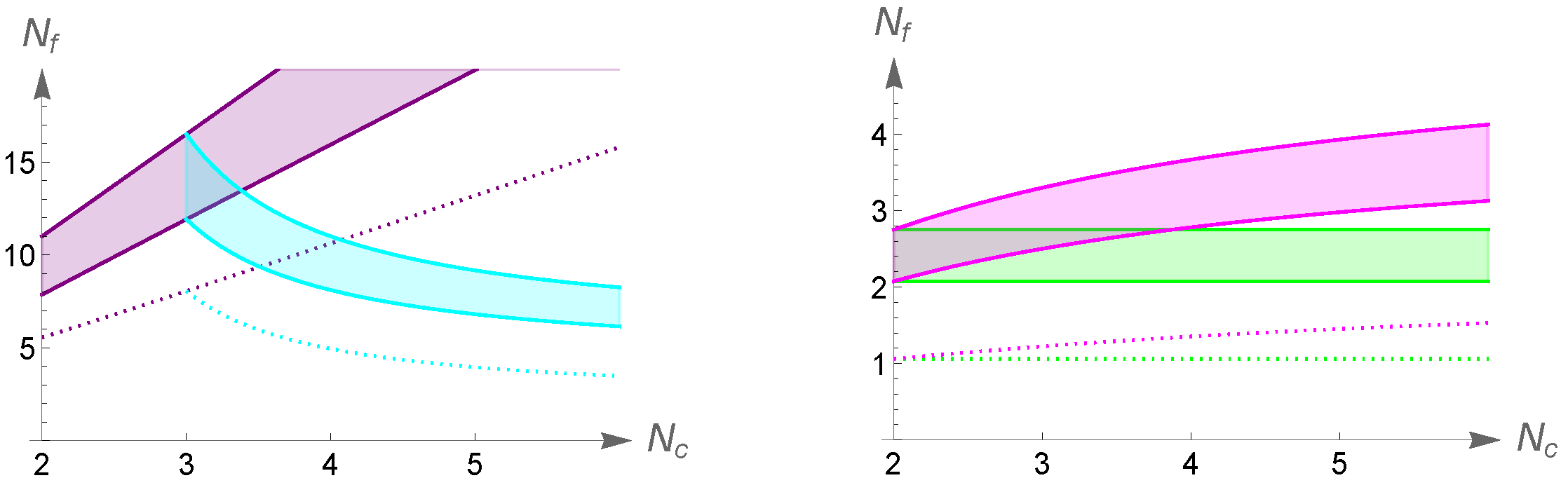
2. Estimates of Gauge Theory Phase Diagrams

In supersymmetric gauge theories, one may approach questions about their nonperturbative behavior using analytic methods [17,18]. We are interested in vacuum phase diagrams of non-supersymmetric theories, and must ultimately apply lattice field theory methods to determine their long distance behavior. In this section, we will apply perturbation theory and estimates of chiral symmetry breaking [19,20] to sketch phase diagrams which provide guide for nonperturbative computations.
Starting with large enough number of fermions, so that the theory is not asymptotically free, N f > N f as , where N f as is determined by the zero of the 1-loop coefficient of the beta-function. In this case the screening of matter fields overwhelms the gauge boson antiscreening and the coupling becomes weaker towards the infra-red. The vacuum phase is that of weakly coupled massless gauge bosons and fermions. The electrically charged probe experiences the potential
V el ( r ) 1 r ln ( r Λ UV ) ,
analogously with QED.
The two-loop beta-function is needed to understand the behavior of the theory with N f just below N f as . The perturbative expansion of the beta-function is
β ( g ) = μ d g d μ = β 0 ( 4 π ) 2 g 3 β 1 ( 4 π ) 4 g 5 + ,
where
β 0 = 11 3 C 2 ( G ) 4 3 T ( R ) N f
and the two loop coefficient is
β 1 = 34 3 C 2 2 ( G ) 20 3 C 2 ( G ) T ( R ) N f 4 C 2 ( R ) T ( R ) N f .
In the above equations for general SU( N c ) representation R the generators T R a , a = 1 , , N c 2 1 are normalized via tr ( T R a T R b ) = T ( R ) δ a b and the quadratic Casimir is given by T R a T R b = C 2 ( R ) 𝟙 . Furthermore, the adjoint representation is denoted by G.
Using the expressions for β 0 and β 1 we see first that N f as = 11 C 2 ( G ) / ( 4 T ( R ) ) . Then, for N f < N f as , the first coefficient is positive while the second coefficient will be negative as long as
N f > 34 C 2 ( G ) 2 ( 20 C 2 ( G ) + 12 C 2 ( R ) ) T ( R ) = N f *
Then, for values of N f in the range N f as > N f > N f * the two-loop beta-function may have a zero, β ( g * ) = 0 , at positive coupling
g * 2 = β 0 β 1 ( 4 π ) 2 .
If we treat N f and N c as continuous variables and define
ϵ = ( N f as N f ) / N c ,
then, for small ϵ , the fixed point g * 2 1 and the perturbation theory analysis is valid [21]. At the fixed point the theory is scale invariant and electric probe charges experience the Coulomb force,
V ( r ) 1 r ,
and the vacuum phase is called the non-Abelian Coulomb phase.
Lowering N f at fixed N c , the above analysis implies a fixed point until the value of N f becomes small enough, that the two-loop coefficient of the beta function changes sign. Then the beta function is negative and QCD-like behavior at strong coupling ensues. Of course these arguments extend to values of g * 2 so large that perturbation theory cannot be trusted anymore.
Qualitatively, one is led to expect that there exists a conformal window extending over the values of
N f crit < N f < N f as ,
where N f crit is a lower bound which needs to be estimated taking into account the strong coupling dynamics beyond perturbative beta-function.
To gain a little insight on how N f crit arises, we can search for chiral symmetry breaking solutions of the truncated gap equation for the fermion two-point function. Nontrivial solutions exist only if the coupling is sufficiently large,
α α c = π 3 C 2 ( R ) .
Given a fixed point α * = g * 2 / ( 4 π 2 ) as implied by Equation (9), one argues that the fixed point persists only as long as the critical coupling α c remains larger than the putative fixed point coupling α * . Therefore, based on the two-loop beta function and the constraint from the critical coupling for chiral symmetry breaking, we can derive the estimate for the value of N f at the lower boundary by solving α * = α c to obtain
N f crit = ( 66 C 2 ( R ) + 17 C 2 ( G ) ) C 2 ( G ) 10 T ( R ) ( 3 C 2 ( R ) + C 2 ( G ) )
which lies above the limiting value of N f * implied by the existence of IRFP in the two-loop beta function, β 1 = 0 .
Based on these results, we can draw sketches of phase diagrams for a given fermion representation. It was shown in [22,23] that there are only few higher representations for which the conformal window may exist. Practically these are the fundamental representation (F), the adjoint (G) and the two-index symmetric ( 2 S ) and antisymmetric ( 2 A S ) representations. The relevant group theory factors are given in Table 1 for the gauge group SU( N c ).
In the left panel of Figure 1 we show the phase diagrams for the fundamental representation and two-index antisymmetric representation and in the right panel the corresponding diagram for the adjoint representation and the two-index symmetric representations.
For N c = 3 the two-index antisymmetric representation coincides with the antifundamental representation and for N c = 2 the two-index symmetric representation coincides with the adjoint representation. The conformal windows of different representations show very different dependencies on the number of flavors: For fundamental representation the conformal window lies at relatively large number of flavors which increases with increasing N c . For two-index antisymmetric representation the location of the conformal window moves to lower number of flavors as N c is increased, but remains above N f = 5 in the limit N c . For two-index symmetric representation the conformal window moves toward larger N f as N c is increased, but the dependecy is very mild: in this case the conformal window is always below N f = 5 . For the adjoint representation the dependency is most simple as the conformal window lies between constant values of N f for any N c .
The phase diagrams in Figure 1 show what one should qualitatively expect, but quantitatively this must be explored using lattice simulations. If the behaviors inferred from these qualitative estimates were confirmed in first principle studies, they could be used to indicate best candidate models to underlie e.g., dynamical electroweak symmetry breaking.

3. The Lattice Formulation

We now turn to the lattice implementation which allows a study of the phase diagrams established in the previous section. We discuss in detail the particular lattice discretization, which we have used in the investigations whose results we will then discuss in the next section. In this section we first describe the lattice action and then the methodology which can be applied to measure the evolution of the coupling and the anomalous dimension of the quark mass operator as well as the anomalous dimension of the leading irrelevant operator i.e., the slope of the beta-function at the critical point.

3.1. The Lattice Action

One of the main issues when applying lattice methods to theories which may be different than QCD is that the methods known to work well for QCD may not be directly applicable. This is particularly true for theories with IRFP: the coupling will evolve very slowly, and one must learn to deal with strong coupling over much wider range of scales than in QCD where asymptotic freedom sets in precociously.
Our computations are based on the lattice model defined by the action
S = ( 1 c g ) S G ( U ) + c g S G ( V ) + S F ,
where U and V denote, respectively, the unsmeared and smeared gauge link matrices. To define the smeared gauge links the hypercubic truncated stout smearing (HEX) is used.
The smearing leads to reduction of discretization errors and allows simulations at large couplings. It was observed in [24], that using partially smeared action enables simulations at stronger physical couplings, and the mixing is quantified by the parameter c g in the above action. The properties of the gauge action are not sensitive to the precise value of c g , and for concreteness we choose c g = 0.5 .
The gauge action above is
S G ( U ) = β L x ; μ < ν 1 1 2 Tr U x , μ U x + μ ^ , ν U x + ν ^ , μ U x , ν ,
where β L = 2 N c / g 0 2 .
For the fermions we use the Wilson–clover fermion action
S F = a 4 x [ ψ ¯ ( x ) ( i D W + m 0 ) ψ ( x ) + a c sw ψ ¯ ( x ) i 4 σ μ ν F μ ν ( x ) ψ ( x ) ] ,
where D W is the standard Wilson Dirac operator. The gauge link matrices contained in S F are constructed from smeared link matrices V in appropriate representation corresponding to fermions.
In addition to the bare coupling β L and the mixing coefficient c g , the lattice action is parametrized by the hopping parameter κ = 1 / ( 2 m 0 + 8 ) and the Sheikholeslami–Wohlert clover coefficient c sw . For smeared gauge links, it is expected [24,25,26] that the tree-level value c sw = 1 is a good approximation. We therefore choose c sw = 1 and note that in principle the validity of this assumption can be verified by measuring its non-perturbative value using the Schrödinger functional tuning method [27] at small volume.
The set of boundary conditions we use are defined as follows: In the spatial boundaries the fields are taken periodic. At the temporal boundaries x 0 = 0 and x 0 = L we use Dirichlet boundary conditions, setting fermion fields to zero and gauge link matrices to unity, U = V = 1 . There are slight exceptions to these when using the Schrödinger functional method for the measurement of the running coupling; we discuss this in more detail below.
The hopping parameter κ is fixed to the critical value κ c by tuning the theory to the chiral limit where the quark mass M ( t = L / 2 ) vanishes. This quark mass is determined using the PCAC relation [28],
a M ( t ) = 1 4 ( t * + t ) f A ( t ) f P ( t ) .
Here, the pseudoscalar current and density correlation functions are
f A ( t ) = a 6 y , z A 0 a ( x , t ) ζ ¯ ( y ) γ 5 λ a ζ ( z )
f P ( t ) = a 6 y , z P a ( x , t ) ζ ¯ ( y ) γ 5 λ a ζ ( z ) ,
where ζ and ζ ¯ are boundary quark sources at x 0 = 0 , and the axial current and density can be expressed as
A μ a ( x ) = ψ ¯ ( x ) γ μ γ 5 λ a ψ ( x )
P a ( x ) = ψ ¯ ( x ) γ 5 λ a ψ ( x )
Here, λ a is an appropriate generator acting on the flavour indices of the quark fields.
In practice, for an analysis at each different value of N c , N f and R, the critical values κ c ( β L ) is determined on one of the largest lattices considered and these same values are then used for all lattices. The resulting errors in the determined mass are on the level of 10 5 and compatible with M = 0 .

3.2. Measurement of the Coupling

There are two methods which have been widely applied to measure the scale evolution of the coupling. These are the Schrödinger functional [29,30,31], i.e., the background field method, and the gradient flow method [32,33]. We now briefly discuss each of them in turn and then explain how the running of the coupling is quantified using the step scaling method.

3.2.1. Schrödinger Functional Method

The Schrödinger functional is the propagation amplitude from some field configuration at boundary x 0 = 0 to another configuration at x 0 = L . The spatial boundaries are taken to be periodic for gauge fields and periodic up to a global phase for fermions.
To set up the measurement of the coupling, the values of the gauge link matrices at the temporal boundaries must be such that they generate a constant background field configuration of least action. Schematically, the boundary fields are parametrised by dimensionless parameters; let us denote the collection of such parameters as η . Then the non-perturbative definition of the coupling is, schematically,
Γ η | η = η 0 = k g 2 ,
where Γ is the effective action and the normalization k is a known function which depends on L / a and the parameter η , and determined so that the above definition matches with the perturbative evaluation. The details of the above description depends on the on the underlying gauge field; see e.g., [27].
In our explicit examples, we consider gauge group SU(2) and then the gauge link boundary matrices depend only on one parameter. Explicitly, they are given by
U i ( x , t = 0 ) = e i η σ 3 a / L ,
U i ( x , t = L ) = e i ( π η ) σ 3 a / L
with η = 0.25 π . Furthermore, in this case the fermion fields are set to zero at the temporal boundaries and have twisted periodic boundary conditions in the spatial directions: ψ ( x + L i ^ ) = exp ( i π / 5 ) ψ ( x ) .

3.2.2. Gradient Flow Method

An alternative definition of the running coupling is based on the Yang–Mills gradient flow method [32,33,34,35]. To set up this method, a fictious new coordinate, the flow time t is introduced together with a gauge field B μ ( x ; t ) related to the original continuum gauge field A μ such that B μ ( x ; t = 0 ) = A μ ( x ) . With this initial condition, this new field is evolved by the flow equation
t B μ = D ν G ν μ ,
where G μ ν ( x ; t ) is the field strength of B μ and D μ = μ + [ B μ , · ] .
To leading order in perturbation theory in SU(N) gauge theory, the field strength evolves as [32]
E ( t ) = 1 4 G μ ν G μ ν ( t ) = 3 ( N 2 1 ) g 0 2 128 π 2 t 2 + O ( g 0 4 ) .
The flow removes the UV divergences systematically, by smoothing the gauge field over the radius r 8 t , and automatically renormalizes gauge invariant observables [36]. Hence, one can define the coupling at scale μ = 1 / 8 t nonperturbatively as
g GF 2 ( μ ) = 128 π 2 3 ( N 2 1 ) t 2 E ( t ) | t = 1 / 8 μ 2 .
To leading order, this matches with perturbation theory.
On the lattice, the continuum flow field is replaced by the lattice link variables U μ ( x ; t ) which are evolved according to
t U μ ( x ; t ) = g 0 2 U μ ( x ; t ) S GF [ U ] U μ ( x ; t )
with the initial condition U μ ( x ; t = 0 ) = U μ ( x ) . The flow evolution action action S GF needs to be chosen, and we use the tree-level improved Lüscher–Weisz pure gauge theory action [37]. There is also choice of discretization when measuring observables for E ( t ) , and we use the clover discretization in our analysis.
To render the coupling defined in Equation (27) free of both lattice artifacts and finite volume effects, the scale needs to be limited into a regime 1 / L μ 1 / a . The lattice size is therefore related to the renormalization scale by defining a dimensionless parameter c t as described in Refs. [38,39,40]:
μ 1 = c t L = 8 t .
Ref. [40] suggests a range of c t = 0.3–0.5 for the SF scheme. Within this range the cutoff effects, statistical variance and boundary effects [41], are reasonably small. In order to minimize the effects of the fixed boundaries at x 0 = 0 and L, we measure the expectation value of the gauge field energy (26) only on the central time slice x 0 = L / 2 .

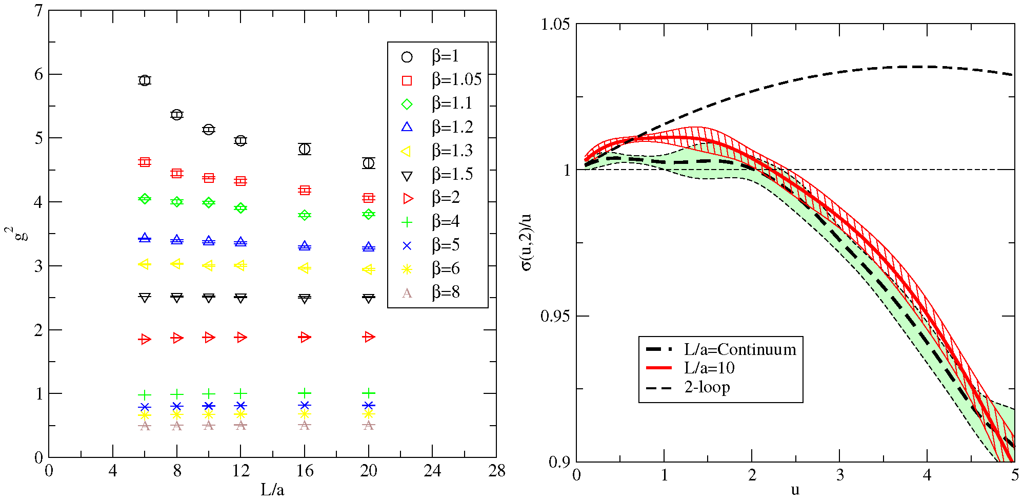
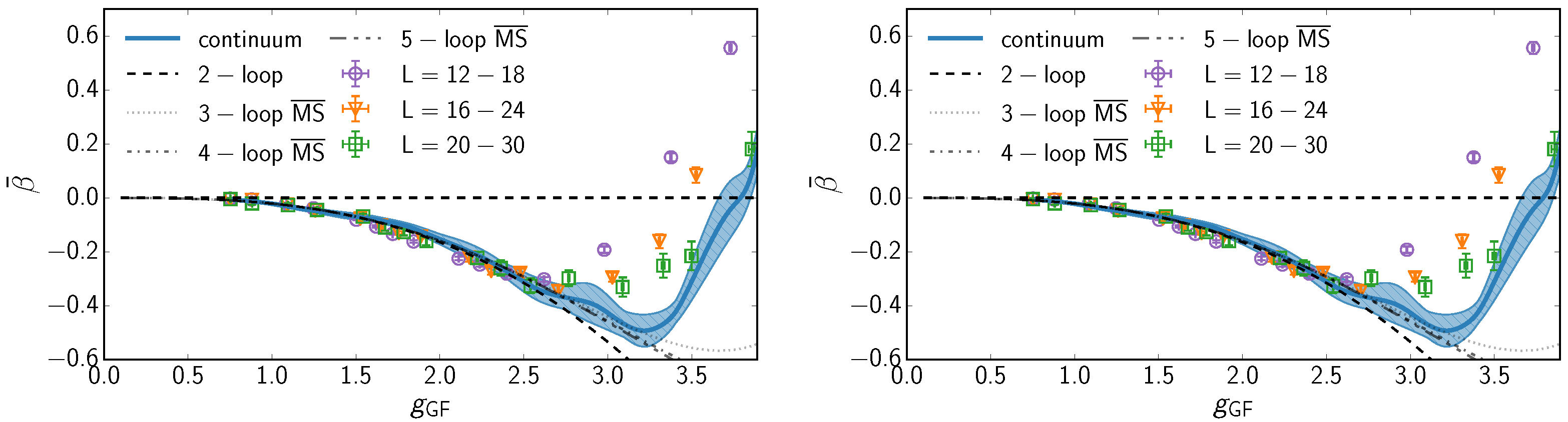
3.3. Step Scaling Analysis

Using either definition of the coupling, its evolution is quantified using the finite lattice spacing step scaling function Σ ( u , s , L / a ) and its continuum limit σ ( u , s ) introduced in Ref. [29]. It describes the change of the measured coupling when the linear size of the system is increased from L to s L , while keeping the bare coupling g 0 2 (and hence the lattice spacing) constant:
Σ ( u , s , L / a ) = g GF 2 ( g 0 2 , s L / a ) g GF 2 ( g 0 2 , L / a ) = u
σ ( u , s ) = lim a / L 0 Σ ( u , s , L / a ) ,
where u denotes g GF 2 as measured from the smaller volume. Often used choice is s = 2 .
The step scaling function is related to the β -function by
2 ln ( s ) = u σ ( u , s ) d x x β ( x ) .
Close to the fixed point, where the running is slow and | β | small, we can approximate the β -function by
β ( g ) β ¯ ( g ) = g 2 ln ( s ) 1 σ ( g 2 , s ) g 2 .
The estimating function β ¯ ( g ) is exact at a fixed point but deviates from the actual β -function as | g g * | becomes large.

3.4. Determination of Anomalous Dimensions

3.4.1. The Fermion Mass Anomalous Dimension

The mass anomalous dimension, γ = d ln m q / d ln μ , can be determined by several different methods. We describe here the step scaling method, which is based on the use of Dirichlet boundary conditions and measurement of the running of the pseudoscalar density renormalization constant [42,43]
Z P ( L ) = N c f 1 f P ( L / 2 ) ,
where the correlation function f P ( t ) is given in Equation (19) and is normalized using the boundary-to-boundary correlator
f 1 = a 12 N c L 6 u , v , y , z ζ ¯ ( u ) γ 5 λ a ζ ( v ) ζ ¯ ( y ) γ 5 λ a ζ ( z ) ,
where ζ and ζ ¯ are boundary fields at x 0 = L .
Now we can define the mass step scaling function as [42]
Σ P ( u , s , L / a ) = Z P ( g 0 , s L / a ) Z P ( g 0 , L / a ) g 2 ( g 0 , L / a ) = u
σ P ( u , s ) = lim a / L 0 Σ P ( u , s , L / a ) .
We choose s = 2 and find the continuum step scaling function σ P by measuring Σ P at L / a = 6 , 8 , 10 and 12 and performing a quadratic extrapolation.
The mass step scaling function is related to the anomalous dimension γ by [43]
σ P ( u , s ) = u σ ( u , s ) d 0 / ( 2 b 0 ) exp u σ ( u , s ) d x γ ( x ) β ( x ) d 0 b 0 x ,
where b 0 = β 0 / ( 16 π 2 ) in terms of the one-loop coefficient β 0 of the beta function and d 0 is the corresponding one-loop coefficient for the anomalous dimension, γ 1 - loop = d 0 g 2 .
Close to the fixed point, expression (38) simplifies considerably: if we denote the function estimating the anomalous dimension γ ( u ) by γ ¯ ( u ) , we have
log σ P ( g 2 , s ) γ ¯ ( g 2 ) μ s μ d μ μ = γ ¯ ( g 2 ) log s ,
γ ¯ ( g 2 ) = log σ P ( g 2 , s ) log s .
The estimator γ ¯ ( g 2 ) is exact at a fixed point g 2 = g * 2 , where β ( g 2 ) vanishes, and deviates from the actual anomalous dimension when β is large. We denote the anomalous exponent at the fixed point with γ * = γ ¯ ( g * 2 ) = γ ( g * 2 ) .
We note that the anomalous dimension of the fermion mass can also be inferred from the scaling of the spectral density of the massless Dirac operator [44]. The explicit calculation of the eigenvalue distribution is numerically costly, but recent advances in applications of stochastic methods [45] have made the mode number of the Dirac operator numerically accessible. This quantity allows the determination of the mass anomalous dimension [46].
Yet another way to access γ * is via the spectrum: if the IR behavior of the theory is governed by a nontrivial fixed point, the hadron masses scale towards zero as
M H m q 1 / ( 1 + γ * ) .
Provided sufficiently precise measurement of the spectrum, this would allow for the determination of γ * .

3.4.2. The Leading Irrelevant Exponent

The leading irrelevant exponent of the coupling γ g is defined as the slope of the β -function. As we have discussed in the previous subsection, on the lattice the evolution of the coupling is measured with the step scaling function. In the vicinity of the fixed point g * , the approximate result of Equation (33) holds. This can then in turn be related to the slope γ g * as follows:
β ( g ) = μ d g d μ β ¯ ( g ) = γ g * ( g g * ) .
This allows one to determine γ g * from the measurement of the beta-function.

4. Case Study: SU(2) Gauge Theory with Fermions on the Lattice

In SU(2) gauge theory the interesting fermion representations are the fundamental and the adjoint, which coincides in two-color case with the two-index symmetric representation. In the following subsections, we will discuss separately the numerical results we have obtained for the lattice model described in the previous section with fermions either in the adjoint [47,48,49,50] or fundamental representation [51,52,53,54]. For theories whose infrared behavior is governed by such nontrivial fixed point, we have also investigated scheme independent critical exponents [49,52,53,54].
The simulations are done using the hybrid Monte Carlo (HMC) algorithm with the 2nd order Omelyan integrator [55,56] and the chronological initial condition for the fermion matrix inversion [57]. The length of the trajectory is fixed to 2 units and the step size is tuned so that the acceptance rate is at least 80%. The measurements are taken after every trajectory and the number of trajectories in each simulation varies up to 200,000. The fermion matrix inversion is acclelerated using the Hasenbusch method [58,59].

4.1. Fermions in the Adjoint Representation

The first consistent study of SU(2) gauge theory with adoint representation fermions was given in [47,48]. In the first of these two papers, the vacuum spectrum of the theory was measured. While the results of [47], compatibly with an earlier investigation [60], seemed to suggest that with adjoint matter both the vector and pseudoscalar masses scale to zero linearly with the quark mass, this could be an artifact arising from the finite size of the system. Only measuring directly the running of the coupling [48] and establishing the existence of the infrared fixed point would strengthen the conclusion that the results on the spectra were probing the physical vacuum phase of the theory. See also [61,62,63]. The measurements of the spectra were extended to gluonic bound states in [64,65].
Our measurement of the coupling is here via the Schrödinger functional and the measured values of g 2 ( L / a , β L ) are shown in the left panel of Figure 2. Here, to define the step scaling function, we use s = 2 and obtain the continuum limit from measurements at L / a = 6 , 8 and 10, pairing these with lattices with L / a = 12 , 16 and 20.
The step scaling function in (30) must be extrapolated to continuum. To do this properly, requires that the measurements at different L / a and 2 L / a -pairs are done at same value of u = g 2 ( g 0 2 , L / a ) . However, the measurements of g 2 are done at a fixed set of bare couplings, β L = 4 / g 0 2 . To relate the couplings on different systems, we interpolate the coupling g 2 ( g 0 2 , L / a ) in order to take the continuum limit.
We use here a rational interpolating function [51]
g 2 ( g 0 2 , L / a ) = g 0 2 1 + i = 1 n a i g 0 2 1 + i = 1 m b i g 0 2
with n = m = 3 . This choice of values is based on minimization of the combined χ 2 over the degrees of freedom. To study the stability of the interpolation one repeats the analysis after reducing n or m by one.
With the interpolating function so determined, the step scaling may be calculated at any value of u = g 2 ( g 0 2 , L / a ) within the interpolation range. This then enables us to obtain the continuum limit using the available three L / a -values. The result is extrapolated to continuum by fitting a function of the form
Σ ( u , 2 , L / a ) = σ ( u , 2 ) + c ( u ) L / a 2 .
For consistent error propagation, the data is divided into 40 jackknife blocks and the analysis is perform separately on the blocks.
The final continuum extrapolated σ ( u , 2 ) / u is shown in the right panel of Figure 2, where also the step scaling function Σ ( u , 2 , 10 ) is obtained from the largest volume alone. Due to the too large values of Σ at small volumes and weak coupling, the continuum limit at small couplings deviates significantly from the perturbative value. Therefore, we expect the L / a = 10 result to represent better the true continuum result than the extrapolated result. For values u 2.5 of the coupling, the agreement between the continuum limit and L/a=10 result is remarkable.
These results indicate the existence of a fixed point. With the continuum extrapolated result the fixed point is close to g * 2 = 2 3 , while using only L / a = 10 results implies that the fixed point is at g * 2 = 2.2 ( 2 ) 0.4 + 0.6 . In the latter result, the first error estimate gives the statistical error and the second includes estimated systematic error from the rational interpolation. It should be noted that the continuum limit result implies only that the fixed point is somewhere below g 2 3 ; see the right panel of Figure 2.
To evaluate the mass step scaling, we proceed similarly as in the analysis of the running coupling. We use an interpolating function to fit the data, and in this case a simple polynomial function is sufficient,
Z P ( β L , L / a ) = 1 + i = 1 n c i g 0 2 i .
In this case the optimal χ 2 over degrees of freedom is given by n = 5 . The systematic error from this step is estimated by reducing n by one and repeating the analysis.
We calculate the mass step scaling function Σ P ( u , s , L / a ) at L / a = 6 , 8 , 10 and 12. The value for the coupling u = g 2 is obtained from the rational fit in Equation (43). Finally, we calculate the estimating function γ ¯ ( u , a / L ) and find the continuum limit γ ¯ ( u ) by fitting to a function of the form γ ¯ ( u , a / L ) = γ ¯ ( u ) + c ( u ) ( a / L ) 2 .
This procedure results to the value of the anomalous dimension at the fixed point as γ * = 0.2 ± 0.03 , where the dominant uncertainty comes from the location of the fixed point, g * 2 2 . 5 0.3 + 0.5 . To compare with other computations, we note that in Ref. [24], using the same scheme, a larger result ( γ * 0.31 ( 6 ) ) was obtained. A different method applied in Ref. [66], led to a result γ * 0.37 ( 2 ) .

4.2. Fermions in the Fundamental Representation

In this case, the running coupling is defined by the Yang–Mills gradient flow method [33,34,35]. We focus on theories with N f = 6 and N f = 8 fermion flavors for which the results indicate existence of an IRFP.
For N f = 6 we use lattices of size L = 8 , 10, 12, 16, 18, 20, 24 and 30. These allow for step scaling analysis using either s = 2 or s = 3 / 2 , and we use the latter choice as it allows for more pairs of larger lattices. For N f = 8 we use L = 6 , 8, 10, 12, 16, 20, 24 and 32, and scaling s = 2 .
In the simulations, the gradient flow is evolved with Lüscher–Weisz action and the clover definition of the energy density is used. In the scale setting the parameter value c t = 0.3 ( c t = 0.4 ) is used for N f = 6 ( N f = 8 ). In the original work we also investigated the systematic errors by varying the discretizations of the flow and observables and also the value of c t .
To quantify the running of the coupling, we applied the step scaling analysis as in the case of the adjoint representation: the measured results were interpolated using a polynomial (rational) fit for N f = 6 ( N f = 8 ). The lattice results were extrapolated to continuum assuming leading dependence on the lattice spacing as O ( a 2 ) .
Regarding this continuum extrapolation we note that since we are not using perfectly improved observables and actions in our gradient flow [67], these source some of the cutoff effects in the coupling g GF 2 . In order to minimize these cutoff effects at the continuum limit, we add a tunable O ( a 2 ) correction τ 0 to the gradient flow coupling, as suggested in Ref. [68]:
g GF 2 = t 2 N E ( t + τ 0 a 2 ) = t 2 N E ( t ) + t 2 N E ( t ) t τ 0 a 2 + O ( a 4 ) .
In practice we use
τ 0 = C ln ( 1 + 2 g GF 2 ) ,
where C = 0.025 for N f = 6 and C = 0.06 for N f = 8 . The results of the measurements are summarized in Figure 3.
From the measurement of the beta-function we can obtain the leading irrelevant exponent γ g * as described in Equation (42). Using the interpolated couplings, the behavior of the coupling near the fixed point is smooth enough to allow determination of γ g * = 0.648 ( 97 ) 0.1 + 0.16 , where the first set of errors implies the statistical errors with the parameters used in Ref. [53], and the second set of errors gives the variance between all measured discretizations. When the values of c t were varied, the γ g * measurements remained consistent with each other, within the errors, indicating the scheme independence of this quantity.
However, we can also directly interpolate the finite volume β ¯ ( g ) -function (42) (where σ ( g 2 , s ) is substituted with Σ ( g 2 , L / a , s ) ), instead of the measured couplings. For the γ g * measurement, this reproduces the value of γ * obtained above. Carrying out this procedure for N f = 8 we obtain γ g * = 0.19 ( 8 ) 0.09 + 0.21 .
We have also measured the anomalous dimension of the fermion mass operator using step scaling and the spectral density methods. The results are γ m * = 0.283 ( 1 ) ± 0.01 for N f = 6 and γ m * = 0.15 ± 0.02 for N f = 8 . The two methods seem consistent with each other and for six flavor theory we have shown consistency with also the value extracted from the vacuum spectrum.

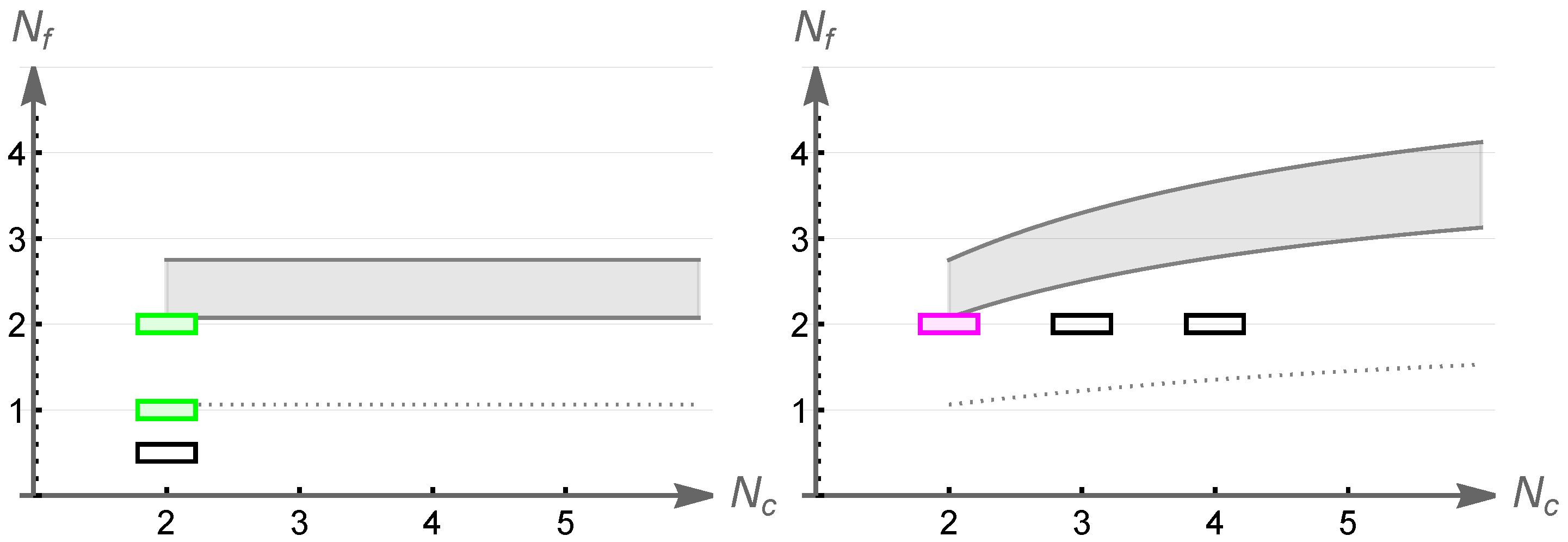
5. Overview of Results for Different Gauge Groups

Next, we present a brief overview of the current results for different fermion representations which have been considered for SU( N c ) gauge groups. These results have been obtained with different lattice discretizations, in particular considering the fermion action. We do not explain the features of these in detail, but only collect the continuum results as stated in the literature.
Starting with the fundamental representation, the summary of the results is presented in Figure 4. The shaded grey band shows the conformal window expected on the basis of two-loop beta-function supplemented with the critical coupling for chiral symmetry breaking from the gap equation analysis (see Section 2). The open rectangles correspond to N f -values for which lattice computations suggest chiral symmetry breaking at low energies and the colored rectangles to values of N f for which a fixed point has been observed.
The results for SU(2) gauge theory the current lattice results indicate that the theory with N f = 2 breaks chiral symmetry [69,70] as does the theory with N f = 4 flavors [51,71]. As we have already discussed in Section 4, the theory with N f = 6 has a fixed point [53,54]. Consistently with this, also theories with N f = 8 flavors [52] and N f = 10 flavors [51] have an IRFP.
For SU(3) gaguge theory, the lattice results in [72] show that from N f = 2 to N f = 6 chiral symmetry is broken. In this study, as N f increases towards N f = 6 the chiral condensate is observed to be enhanced, which is interpreted as a signal for the approach to the boundary of the conformal window. Furthermore, also N f = 8 theory was reported to break chiral symmetry in [73,74,75,76] and similar result was obtained for N f = 9 theory in [77].
For SU(3) gauge theory and N f = 10 fermions the current status has not been consistently established. In [78] the running was observed to slow towards the infrared, and this was interpreted as evidence in favor of a fixed point. In [79] the observed spectrum is consistent with IR conformality, but cannot rule out the possibility of spontaneous chiral symmetry breaking at scales below the the infrared cutoff. Infrared conformality was also suggested in [80,81] while spontaneous chiral symmetry breaking was observed in [82]. Assuming that this theory has a fixed point, the value of the quark mass anomalous dimension γ * can be inferred. The analysis in [79] yields γ * = 1.1 .
For N f = 12 as well the infrared behavior has not been established without doubts. Early work in [73] suggested that the infrared behavior is governed by an IRFP. This result is supported by the results reported in [83,84] and similar conclusion was suggested in [85]. However, no sign of a fixed point in the twelve flavor SU(3) theory was observed in [86,87]. If this theory has a fixed point, the the computation in [88] yields the value γ * = 0.41 for the anomalous dimension of the quark mass operator. Similar result has been obtained also in [89,90] while slightly smaller values were reported in [91,92,93]
Similar compilation of results is presented for adjoint and two-index symmetric representation fermion in Figure 5.
Lattice simulations exist for SU(2) gauge theory N f = 1 and 2 Dirac fermions in the adjoint representation. For both of these value the IRFP has been established. The case N f = 1 is treated in [94] while N f = 2 has been studied by several independent computations [24,47,48,49,50,63,95,96] all leading to conclusions consistent with each other; this theory provides the most clean example of a system with an IRFP. For SU(2) theory also N f = 1 / 2 and 3 / 2 can be simulated [96] as these correspond to Majorana fermions. For these, N f = 3 / 2 has an IRFP while N f = 1 / 2 is observed to be outside the conformal window consistently with the fact that this theory is N = 1 super-Yang–Mills theory for which no fixed point should exist.
Two adjoint flavors for N c > 2 would be very interesting to investigate since the analytic estimates for the phase diagram suggest independence on the number of colors. Currently there exists only one study in SU(3) with two adjoints [97]. The results do not allow to confirm or rule out an IRFP in this theory.
Finally, the theory with N f = 2 flavors in the two-index symmetric representation has been studied for different values of N c . The case N c = 2 coincides with the adjoint representation and is therefore inside the conformal window. The theory with N c = 3 seems to be outside the conformal window [98,99], but possibly only slightly as evidenced by the existence of a light 0 + + scalar meson state [100]. Finally, for N c = 4 no IRFP has been observed [101].
For three colors the phase diagram of two-index antisymmetric representation would be the same as for the fundamental representation. Beyond N c = 3 , for the two-index antisymmetric representation there has been only one study [97] in SU(4) gauge theory with N f = 6 fermions and the results do not allow to confirm or rule out an IRFP in this theory.

6. Conclusions and Outlook

In this review we have considered motivations for lattice calculations of gauge theory phase diagrams as a function of the number of colors, flavors and fermion representations. We have discussed in detail state of the art computations in SU(2) gauge theory with either fundamental or adjoint fermion matter and reviewed the current results for SU(2) and other SU( N c ) gauge theories.
Phase diagrams constitute a fundamental piece of information and insight on the dynamics of gauge theories. While interesting on their own, they are an essential tool in identifying phenomenologically interesting theories which can be utilized in building candidate theories beyond the Standard Model. Possible applications are e.g., in dynamical electroweak symmetry breaking [102] or dark matter [16]. Towards the former, near-conformal theories may explain the lightness of the Higgs in relation to the rest of the composite spectrum [103] which remains so far unobserved at collider experiments. Towards the latter form factors of composite states interacting with ordinary matter may explain why models where large enough relic density can be produced at high energy remain hidden at low energy scatterings.
Based on the results we have described here, there are many further avenues to pursue, and initial investigations along some of them have already started. While the existence and properties of an IRFP is most robustly uncovered by measurement of the running coupling, the vacuum spectra is another important observable. This is particularly interesting for theories near the lower boundary of the conformal window, since the spectrum provides insight into identification of phenomenologically interesting theories. There is already accumulated evidence that the near-conformal theories do indeed feature a light scalar state, see e.g., [81,100].
A natural and interesting further development would be to study theories with multiple fermion representations. For initial investigations towards this direction see e.g., [104,105,106]. A related development is to allow the fermions to have different mass scales [81]. This leads to decoupling and may lead to realisation of walking theories.
Finally, there has been recent development in simulating theories with very large number of fermions, so that the theory is realized in the non-asymptotically free but infrared free phase. It has been shown that such simulations can be done and the measured running coupling matches consistently with perturbation theory in the weak coupling regime [107]. Moreover, the vacuum spectrum has been measured in this theory [108], and the result is consistent with infrared free behavior.
Future research on unveiling the phase diagrams and extending the research goals along the lines we have discussed above should allow for more insight into the gauge theory dynamics at strong coupling and shed more light on their phenomenological applications.

Data Availability Statement

Not applicable.

Acknowledgments

The work was supported by the Academy of Finland grants 320123, 319066, 308791 and 310130.

Conflicts of Interest

The authors declare no conflict of interest.

References

  1. Yang, C.N.; Mills, R.L. Conservation of Isotopic Spin and Isotopic Gauge Invariance. Phys. Rev. 1954, 96, 191–195. [Google Scholar] [CrossRef]
  2. Gross, D.J.; Wilczek, F. Ultraviolet Behavior of Nonabelian Gauge Theories. Phys. Rev. Lett. 1973, 30, 1343–1346. [Google Scholar] [CrossRef] [Green Version]
  3. Politzer, H.D. Reliable Perturbative Results for Strong Interactions? Phys. Rev. Lett. 1973, 30, 1346–1349. [Google Scholar] [CrossRef] [Green Version]
  4. Smith, C.H.L. Inelastic lepton scattering in gluon models. Phys. Rev. D 1971, 4, 2392. [Google Scholar] [CrossRef] [Green Version]
  5. Gross, D.J. How to Test Scaling in Asymptotically Free Theories. Phys. Rev. Lett. 1974, 32, 1071. [Google Scholar] [CrossRef]
  6. Feynman, R.P. The behavior of hadron collisions at extreme energies. Conf. Proc. C 1969, 690905, 237–258. [Google Scholar]
  7. Brock, R.L.; Collins, J.; Huston, J.; Kuhlmann, S.E.; Mishra, S.; Morfín, J.G.; Olness, F.I.; Owens, J.; Pumplin, J.; Iu, J.W.; et al. Handbook of Perturbative QCD, Version 1.1. Rev. Mod. Phys. 1995, 67, 157–248. [Google Scholar]
  8. Particle Data Group; Zyla, P.A.; Barnett, R.M.; Beringer, J.; Dahl, O.; Dwyer, D.A.; Groom, D.E.; Lin, C.-J.; Lugovsky, K.S.; Pianori, E.; et al. Review of Particle Physics. Prog. Theor. Exp. Phys. 2020, 2020, 083C01. [Google Scholar] [CrossRef]
  9. Wilson, K.G. Confinement of Quarks. Phys. Rev. D 1974, 10, 2445–2459. [Google Scholar] [CrossRef]
  10. DeGrand, T.; Detar, C.E. Lattice Methods for Quantum Chromodynamics; World Scientific: Singapore, 2006. [Google Scholar]
  11. Weinberg, S. Implications of Dynamical Symmetry Breaking. Phys. Rev. D 1976, 13, 974–996. [Google Scholar] [CrossRef] [Green Version]
  12. Susskind, L. Dynamics of Spontaneous Symmetry Breaking in the Weinberg-Salam Theory. Phys. Rev. D 1979, 20, 2619–2625. [Google Scholar] [CrossRef] [Green Version]
  13. Holdom, B. Raising Condensates Beyond the Ladder. Phys. Lett. B 1988, 213, 365–369. [Google Scholar] [CrossRef]
  14. Hill, C.T.; Simmons, E.H. Strong Dynamics and Electroweak Symmetry Breaking. Phys. Rept. 2003, 381, 235–402, Erratum in Phys. Rept. 2004, 390, 553–554. [Google Scholar] [CrossRef] [Green Version]
  15. Sannino, F. Dynamical Stabilization of the Fermi Scale: Phase Diagram of Strongly Coupled Theories for (Minimal) Walking Technicolor and Unparticles. arXiv 2008, arXiv:0804.0182. [Google Scholar]
  16. Kribs, G.D.; Neil, E.T. Review of strongly-coupled composite dark matter models and lattice simulations. Int. J. Mod. Phys. A 2016, 31, 1643004. [Google Scholar] [CrossRef]
  17. Intriligator, K.A.; Seiberg, N. Lectures on supersymmetric gauge theories and electric-magnetic duality. Nucl. Phys. B Proc. Suppl. 1996, 45BC, 1–28. [Google Scholar] [CrossRef] [Green Version]
  18. Peskin, M.E. Duality in supersymmetric Yang-Mills theory. arXiv 1997, arXiv:hep-th/9702094. [Google Scholar]
  19. Appelquist, T.; Lane, K.D.; Mahanta, U. On the Ladder Approximation for Spontaneous Chiral Symmetry Breaking. Phys. Rev. Lett. 1988, 61, 1553. [Google Scholar] [CrossRef] [PubMed]
  20. Cohen, A.G.; Georgi, H. Walking Beyond the Rainbow. Nucl. Phys. B 1989, 314, 7–24. [Google Scholar] [CrossRef]
  21. Banks, T.; Zaks, A. On the Phase Structure of Vector-Like Gauge Theories with Massless Fermions. Nucl. Phys. B 1982, 196, 189–204. [Google Scholar] [CrossRef]
  22. Sannino, F.; Tuominen, K. Orientifold theory dynamics and symmetry breaking. Phys. Rev. D 2005, 71, 051901. [Google Scholar] [CrossRef] [Green Version]
  23. Dietrich, D.D.; Sannino, F. Conformal window of SU(N) gauge theories with fermions in higher dimensional representations. Phys. Rev. D 2007, 75, 085018. [Google Scholar] [CrossRef] [Green Version]
  24. DeGrand, T.; Shamir, Y.; Svetitsky, B. Infrared fixed point in SU(2) gauge theory with adjoint fermions. Phys. Rev. D 2011, 83, 074507. [Google Scholar] [CrossRef] [Green Version]
  25. Capitani, S.; Durr, S.; Hoelbling, C. Rationale for UV-filtered clover fermions. J. High Energy Phys. 2006, 11, 028. [Google Scholar] [CrossRef] [Green Version]
  26. Shamir, Y.; Svetitsky, B.; Yurkovsky, E. Improvement via hypercubic smearing in triplet and sextet QCD. Phys. Rev. D 2011, 83, 097502. [Google Scholar] [CrossRef] [Green Version]
  27. Luscher, M.; Sommer, R.; Weisz, P.; Wolff, U. A Precise determination of the running coupling in the SU(3) Yang-Mills theory. Nucl. Phys. B 1994, 413, 481–502. [Google Scholar] [CrossRef] [Green Version]
  28. Luscher, M.; Weisz, P. O(a) improvement of the axial current in lattice QCD to one loop order of perturbation theory. Nucl. Phys. B 1996, 479, 429–458. [Google Scholar] [CrossRef] [Green Version]
  29. Luscher, M.; Narayanan, R.; Weisz, P.; Wolff, U. The Schrödinger functional: A Renormalizable probe for nonAbelian gauge theories. Nucl. Phys. B 1992, 384, 168–228. [Google Scholar] [CrossRef] [Green Version]
  30. Jansen, K.; Sommer, R. O(a) improvement of lattice QCD with two flavors of Wilson quarks. Nucl. Phys. B 1998, 530, 185–203, Erratum in Nucl. Phys. B 2002, 643, 517–518. [Google Scholar] [CrossRef] [Green Version]
  31. Della Morte, M.; Frezzotti, R.; Heitger, J.; Rolf, J.; Sommer, R.; Wolff, U.; Alpha Collaboration. Computation of the strong coupling in QCD with two dynamical flavors. Nucl. Phys. B 2005, 713, 378–406. [Google Scholar] [CrossRef] [Green Version]
  32. Lüscher, M. Properties and uses of the Wilson flow in lattice QCD. J. High Energy Phys. 2010, 8, 071, Erratum in J. High Energy Phys. 2014, 3, 092. [Google Scholar] [CrossRef]
  33. Ramos, A. The Yang-Mills gradient flow and renormalization. arXiv 2015, arXiv:1506.00118. [Google Scholar]
  34. Narayanan, R.; Neuberger, H. Infinite N phase transitions in continuum Wilson loop operators. J. High Energy Phys. 2006, 3, 064. [Google Scholar] [CrossRef] [Green Version]
  35. Luscher, M. Trivializing maps, the Wilson flow and the HMC algorithm. Commun. Math. Phys. 2010, 293, 899–919. [Google Scholar] [CrossRef] [Green Version]
  36. Luscher, M.; Weisz, P. Perturbative analysis of the gradient flow in non-abelian gauge theories. J. High Energy Phys. 2011, 2, 051. [Google Scholar] [CrossRef] [Green Version]
  37. Luscher, M.; Weisz, P. On-Shell Improved Lattice Gauge Theories. Commun. Math. Phys. 1985, 97, 59, Erratum in Commun. Math. Phys. 1985, 98, 433. [Google Scholar] [CrossRef]
  38. Fodor, Z.; Holland, K.; Kuti, J.; Nogradi, D.; Wong, C.H. The Yang-Mills gradient flow in finite volume. J. High Energy Phys. 2012, 11, 007. [Google Scholar] [CrossRef] [Green Version]
  39. Fodor, Z.; Holland, K.; Kuti, J.; Nogradi, D.; Wong, C.H. The gradient flow running coupling scheme. arXiv 2012, arXiv:1211.3247. [Google Scholar]
  40. Fritzsch, P.; Ramos, A. The gradient flow coupling in the Schrödinger Functional. J. High Energy Phys. 2013, 10, 008. [Google Scholar] [CrossRef] [Green Version]
  41. Lüscher, M. Step scaling and the Yang-Mills gradient flow. J. High Energy Phys. 2014, 6, 105. [Google Scholar] [CrossRef] [Green Version]
  42. Capitani, S.; Lüscher, M.; Sommer, R.; Wittig, H. Non-perturbative quark mass renormalization in quenched lattice QCD. Nucl. Phys. B 1999, 544, 669–698, Erratum in Nucl. Phys. B 2000, 582, 762–762. [Google Scholar] [CrossRef] [Green Version]
  43. Della Morte, M.; Hoffmann, R.; Knechtli, F.; Rolf, J.; Sommer, R.; Wetzorke, I.; Wolffa, U.; Alpha Collaboration. Non-perturbative quark mass renormalization in two-flavor QCD. Nucl. Phys. B 2005, 729, 117–134. [Google Scholar] [CrossRef] [Green Version]
  44. Del Debbio, L.; Zwicky, R. Hyperscaling relations in mass-deformed conformal gauge theories. Phys. Rev. D 2010, 82, 014502. [Google Scholar] [CrossRef] [Green Version]
  45. Giusti, L.; Luscher, M. Chiral symmetry breaking and the Banks-Casher relation in lattice QCD with Wilson quarks. J. High Energy Phys. 2009, 3, 013. [Google Scholar] [CrossRef] [Green Version]
  46. Patella, A. GMOR-like relation in IR-conformal gauge theories. Phys. Rev. D 2011, 84, 125033. [Google Scholar] [CrossRef] [Green Version]
  47. Hietanen, A.J.; Rantaharju, J.; Rummukainen, K.; Tuominen, K. Spectrum of SU(2) lattice gauge theory with two adjoint Dirac flavours. J. High Energy Phys. 2009, 5, 025. [Google Scholar] [CrossRef]
  48. Hietanen, A.J.; Rummukainen, K.; Tuominen, K. Evolution of the coupling constant in SU(2) lattice gauge theory with two adjoint fermions. Phys. Rev. D 2009, 80, 094504. [Google Scholar] [CrossRef] [Green Version]
  49. Rantaharju, J.; Rantalaiho, T.; Rummukainen, K.; Tuominen, K. Running coupling in SU(2) gauge theory with two adjoint fermions. Phys. Rev. D 2016, 93, 094509. [Google Scholar] [CrossRef] [Green Version]
  50. Rantaharju, J. Gradient Flow Coupling in the SU(2) gauge theory with two adjoint fermions. Phys. Rev. D 2016, 93, 094516. [Google Scholar] [CrossRef] [Green Version]
  51. Karavirta, T.; Rantaharju, J.; Rummukainen, K.; Tuominen, K. Determining the conformal window: SU(2) gauge theory with Nf = 4, 6 and 10 fermion flavours. J. High Energy Phys. 2012, 5, 003. [Google Scholar] [CrossRef] [Green Version]
  52. Leino, V.; Rantaharju, J.; Rantalaiho, T.; Rummukainen, K.; Suorsa, J.M.; Tuominen, K. The gradient flow running coupling in SU(2) gauge theory with Nf = 8 fundamental flavors. Phys. Rev. D 2017, 95, 114516. [Google Scholar] [CrossRef] [Green Version]
  53. Leino, V.; Rummukainen, K.; Suorsa, J.M.; Tuominen, K.; Tähtinen, S. Infrared fixed point of SU(2) gauge theory with six flavors. Phys. Rev. D 2018, 97, 114501. [Google Scholar] [CrossRef] [Green Version]
  54. Leino, V.; Rummukainen, K.; Tuominen, K. Slope of the beta function at the fixed point of SU(2) gauge theory with six or eight flavors. Phys. Rev. D 2018, 98, 054503. [Google Scholar] [CrossRef] [Green Version]
  55. Omelyan, I.P.; Mryglod, I.M.; Folk, R. Symplectic analytically integrable decomposition algorithms: Classification, derivation, and application to molecular dynamics, quantum and celestial mechanics simulations. Comput. Phys. Commun. 2003, 151, 272–314. [Google Scholar] [CrossRef]
  56. Takaishi, T.; de Forcrand, P. Testing and tuning new symplectic integrators for hybrid Monte Carlo algorithm in lattice QCD. Phys. Rev. E 2006, 73, 036706. [Google Scholar] [CrossRef] [Green Version]
  57. Brower, R.C.; Ivanenko, T.; Levi, A.R.; Orginos, K.N. Chronological inversion method for the Dirac matrix in hybrid Monte Carlo. Nucl. Phys. B 1997, 484, 353–374. [Google Scholar] [CrossRef] [Green Version]
  58. Hasenbusch, M.; Jansen, K. Speeding up the Hybrid Monte Carlo algorithm for dynamical fermions. Nucl. Phys. B Proc. Suppl. 2002, 106, 1076–1078. [Google Scholar] [CrossRef] [Green Version]
  59. Hasenbusch, M.; Jansen, K. Speeding up lattice QCD simulations with clover improved Wilson fermions. Nucl. Phys. B 2003, 659, 299–320. [Google Scholar] [CrossRef] [Green Version]
  60. Catterall, S.; Sannino, F. Minimal walking on the lattice. Phys. Rev. D 2007, 76, 034504. [Google Scholar] [CrossRef] [Green Version]
  61. Del Debbio, L.; Patella, A.; Pica, C. Higher representations on the lattice: Numerical simulations. SU(2) with adjoint fermions. Phys. Rev. D 2010, 81, 094503. [Google Scholar] [CrossRef] [Green Version]
  62. del Debbio, L.; Lucini, B.; Patella, A.; Pica, C.; Rago, A. Conformal versus confining scenario in SU(2) with adjoint fermions. Phys. Rev. D 2009, 80, 074507. [Google Scholar] [CrossRef] [Green Version]
  63. Bursa, F.; del Debbio, L.; Keegan, L.; Pica, C.; Pickup, T. Mass anomalous dimension in SU(2) with two adjoint fermions. Phys. Rev. D 2010, 81, 014505. [Google Scholar] [CrossRef] [Green Version]
  64. Patella, A.; del Debbio, L.; Lucini, B.; Pica, C.; Rago, A. Confining vs. conformal scenario for SU(2) with adjoint fermions. Gluonic observables. arXiv 2010, arXiv:1011.0864. [Google Scholar]
  65. Bursa, F.; del Debbio, L.; Henty, D.; Kerrane, E.; Lucini, B.; Patella, A.; Pica, C.; Pickup, T.; Rago, A. Improved Lattice Spectroscopy of Minimal Walking Technicolor. Phys. Rev. D 2011, 84, 034506. [Google Scholar] [CrossRef] [Green Version]
  66. Patella, A. A precise determination of the psibar-psi anomalous dimension in conformal gauge theories. Phys. Rev. D 2012, 86, 025006. [Google Scholar] [CrossRef] [Green Version]
  67. Ramos, A.; Sint, S. Symanzik improvement of the gradient flow in lattice gauge theories. Eur. Phys. J. C 2016, 76, 15. [Google Scholar] [CrossRef] [Green Version]
  68. Cheng, A.; Hasenfratz, A.; Liu, Y.; Petropoulos, G.; Schaich, D. Improving the continuum limit of gradient flow step scaling. J. High Energy Phys. 2014, 5, 137. [Google Scholar] [CrossRef] [Green Version]
  69. Arthur, R.; Drach, V.; Hansen, M.; Hietanen, A.; Pica, C.; Sannino, F. SU(2) gauge theory with two fundamental flavors: A minimal template for model building. Phys. Rev. D 2016, 94, 094507. [Google Scholar] [CrossRef] [Green Version]
  70. Arthur, R.; Drach, V.; Hietanen, A.; Pica, C.; Sannino, F. SU(2) Gauge Theory with Two Fundamental Flavours: Scalar and Pseudoscalar Spectrum. arXiv 2016, arXiv:1607.06654. [Google Scholar]
  71. Amato, A.; Leino, V.; Rummukainen, K.; Tuominen, K.; Tähtinen, S. From chiral symmetry breaking to conformality in SU(2) gauge theory. arXiv 2018, arXiv:1806.07154. [Google Scholar]
  72. Appelquist, T.; Avakian, A.; Babich, R.; Brower, R.C.; Cheng, M.; Clark, M.A.; Cohen, G.T.; Fleming, J.; Kiskis, E.T.; Neil, J.C.; et al. Toward TeV Conformality. Phys. Rev. Lett. 2010, 104, 071601. [Google Scholar] [CrossRef] [PubMed] [Green Version]
  73. Appelquist, T.; Fleming, G.T.; Neil, E.T. Lattice Study of Conformal Behavior in SU(3) Yang-Mills Theories. Phys. Rev. D 2009, 79, 076010. [Google Scholar] [CrossRef] [Green Version]
  74. Appelquist, T.; Brower, R.C.; Fleming, G.T.; Kiskis, J.; Lin, M.F.; Neil, E.T.; Osborn, J.; Rebbi, C.; Rinaldi, E.; Schaich, D.; et al. Lattice simulations with eight flavors of domain wall fermions in SU(3) gauge theory. Phys. Rev. D 2014, 90, 114502. [Google Scholar] [CrossRef] [Green Version]
  75. Hasenfratz, A.; Schaich, D.; Veernala, A. Nonperturbative β function of eight-flavor SU(3) gauge theory. J. High Energy Phys. 2015, 6, 143. [Google Scholar] [CrossRef]
  76. Fodor, Z.; Holland, K.; Kuti, J.; Mondal, S.; Nogradi, D.; Wong, C.H. The running coupling of 8 flavors and 3 colors. J. High Energy Phys. 2015, 6, 019. [Google Scholar] [CrossRef] [Green Version]
  77. Fodor, Z.; Holland, K.; Kuti, J.; Nogradi, D.; Schroeder, C. Chiral symmetry breaking in nearly conformal gauge theories. arXiv 2009, arXiv:0911.2463. [Google Scholar]
  78. Hayakawa, M.; Ishikawa, K.I.; Osaki, Y.; Takeda, S.; Uno, S.; Yamada, N. Running coupling constant of ten-flavor QCD with the Schrödinger functional method. Phys. Rev. D 2011, 83, 074509. [Google Scholar] [CrossRef] [Green Version]
  79. Appelquist, T.; Brower, R.C.; Buchoff, M.I.; Cheng, M.; Cohen, S.D.; Fleming, G.T.; Kiskis, J.; Lin, M.; Na, H.; Neil, E.T.; et al. Approaching Conformality with Ten Flavors. arXiv 2012, arXiv:1204.6000. [Google Scholar]
  80. Hasenfratz, A.; Rebbi, C.; Witzel, O. Gradient flow step-scaling function for SU(3) with ten fundamental flavors. Phys. Rev. D 2020, 101, 114508. [Google Scholar] [CrossRef]
  81. Appelquist, T.; Brower, R.C.; Cushman, K.K.; Fleming, G.T.; Gasbarro, A.D.; Hasenfratz, A.; Jin, X.-Y.; Neil, E.T.; Osborn, J.C.; Rebbi, C.; et al. Near-conformal dynamics in a chirally broken system. Phys. Rev. D 2021, 103, 014504. [Google Scholar] [CrossRef]
  82. Fodor, Z.; Holland, K.; Kuti, J.; Nogradi, D.; Wong, C.H. Fate of a recent conformal fixed point and β-function in the SU(3) BSM gauge theory with ten massless flavors. arXiv 2018, arXiv:1812.03972. [Google Scholar]
  83. Hasenfratz, A.; Schaich, D. Nonperturbative β function of twelve-flavor SU(3) gauge theory. J. High Energy Phys. 2018, 2, 132. [Google Scholar] [CrossRef] [Green Version]
  84. Hasenfratz, A.; Rebbi, C.; Witzel, O. Gradient flow step-scaling function for SU(3) with twelve flavors. Phys. Rev. D 2019, 100, 114508. [Google Scholar] [CrossRef] [Green Version]
  85. Lin, C.J.D.; Ogawa, K.; Ohki, H.; Shintani, E. Lattice study of infrared behaviour in SU(3) gauge theory with twelve massless flavours. J. High Energy Phys. 2012, 8, 096. [Google Scholar] [CrossRef] [Green Version]
  86. Fodor, Z.; Holland, K.; Kuti, J.; Nogradi, D.; Schroeder, C.; Holland, K.; Kuti, J.; Nogradi, D.; Schroeder, C. Twelve massless flavors and three colors below the conformal window. Phys. Lett. B 2011, 703, 348–358. [Google Scholar] [CrossRef] [Green Version]
  87. Fodor, Z.; Holland, K.; Kuti, J.; Mondal, S.; Nogradi, D.; Wong, C.H. Fate of the conformal fixed point with twelve massless fermions and SU(3) gauge group. Phys. Rev. D 2016, 94, 091501. [Google Scholar] [CrossRef] [Green Version]
  88. Appelquist, T.; Fleming, G.T.; Lin, M.F.; Neil, E.T.; Schaich, D.A. Lattice Simulations and Infrared Conformality. Phys. Rev. D 2011, 84, 054501. [Google Scholar] [CrossRef] [Green Version]
  89. Aoki, Y.; Aoyama, T.; Kurachi, M.; Maskawa, T.; Nagai, K.I.; Ohki, H.; Shibata, A.; Yamawaki, K.; Yamazaki, T. Lattice study of conformality in twelve-flavor QCD. Phys. Rev. D 2012, 86, 054506. [Google Scholar] [CrossRef] [Green Version]
  90. DeGrand, T. Finite-size scaling tests for spectra in SU(3) lattice gauge theory coupled to 12 fundamental flavor fermions. Phys. Rev. D 2011, 84, 116901. [Google Scholar] [CrossRef] [Green Version]
  91. Cheng, A.; Hasenfratz, A.; Petropoulos, G.; Schaich, D. Scale-dependent mass anomalous dimension from Dirac eigenmodes. J. High Energy Phys. 2013, 7, 061. [Google Scholar] [CrossRef] [Green Version]
  92. Cheng, A.; Hasenfratz, A.; Liu, Y.; Petropoulos, G.; Schaich, D. Finite size scaling of conformal theories in the presence of a near-marginal operator. Phys. Rev. D 2014, 90, 014509. [Google Scholar] [CrossRef] [Green Version]
  93. Lombardo, M.P.; Miura, K.; da Silva, T.J.N.; Pallante, E. On the particle spectrum and the conformal window. J. High Energy Phys. 2014, 12, 183. [Google Scholar] [CrossRef] [Green Version]
  94. Athenodorou, A.; Bennett, E.; Bergner, G.; Lucini, B. Investigating the conformal behavior of SU(2) with one adjoint Dirac flavor. Phys. Rev. D 2021, 104, 074519. [Google Scholar] [CrossRef]
  95. Del Debbio, L.; Lucini, B.; Patella, A.; Pica, C.; Rago, A. The infrared dynamics of Minimal Walking Technicolor. Phys. Rev. D 2010, 82, 014510. [Google Scholar] [CrossRef] [Green Version]
  96. Lopez, C.; Bergner, G.; Montvay, I.; Piemonte, S. Measurement of the mass anomalous dimension of near-conformal adjoint QCD with the gradient flow. arXiv 2020, arXiv:2011.02815. [Google Scholar]
  97. DeGrand, T.; Shamir, Y.; Svetitsky, B. Near the Sill of the Conformal Window: Gauge Theories with Fermions in Two-Index Representations. Phys. Rev. D 2013, 88, 054505. [Google Scholar] [CrossRef] [Green Version]
  98. DeGrand, T.; Shamir, Y.; Svetitsky, B. Running coupling and mass anomalous dimension of SU(3) gauge theory with two flavors of symmetric-representation fermions. Phys. Rev. D 2010, 82, 054503. [Google Scholar] [CrossRef] [Green Version]
  99. Fodor, Z.; Holland, K.; Kuti, J.; Mondal, S.; Nogradi, D.; Wong, C.H. The running coupling of the minimal sextet composite Higgs model. J. High Energy Phys. 2015, 9, 039. [Google Scholar] [CrossRef]
  100. Fodor, Z.; Holland, K.; Kuti, J.; Wong, C.H. Tantalizing dilaton tests from a near-conformal EFT. arXiv 2019, arXiv:1901.06324. [Google Scholar]
  101. DeGrand, T.; Shamir, Y.; Svetitsky, B. SU(4) lattice gauge theory with decuplet fermions: Schrödinger functional analysis. Phys. Rev. D 2012, 85, 074506. [Google Scholar] [CrossRef] [Green Version]
  102. Cacciapaglia, G.; Pica, C.; Sannino, F. Fundamental Composite Dynamics: A Review. Phys. Rept. 2020, 877, 1–70. [Google Scholar] [CrossRef]
  103. Dietrich, D.D.; Sannino, F.; Tuominen, K. Light composite Higgs from higher representations versus electroweak precision measurements: Predictions for CERN LHC. Phys. Rev. D 2005, 72, 055001. [Google Scholar] [CrossRef] [Green Version]
  104. Ayyar, V.; DeGrand, T.; Golterman, M.; Hackett, D.C.; Jay, W.I.; Neil, E.T.; Shamir, Y.; Svetitsky, B. Spectroscopy of SU(4) composite Higgs theory with two distinct fermion representations. Phys. Rev. D 2018, 97, 074505. [Google Scholar] [CrossRef] [Green Version]
  105. Ayyar, V.; DeGrand, T.; Hackett, D.C.; Jay, W.I.; Neil, E.T.; Shamir, Y.; Svetitsky, B. Finite-temperature phase structure of SU(4) gauge theory with multiple fermion representations. Phys. Rev. D 2018, 97, 114502. [Google Scholar] [CrossRef] [Green Version]
  106. Cossu, G.; del Debbio, L.; Panero, M.; Preti, D. Strong dynamics with matter in multiple representations: SU(4) gauge theory with fundamental and sextet fermions. Eur. Phys. J. C 2019, 79, 638. [Google Scholar] [CrossRef]
  107. Leino, V.; Rindlisbacher, T.; Rummukainen, K.; Sannino, F.; Tuominen, K. Safety versus triviality on the lattice. Phys. Rev. D 2020, 101, 074508. [Google Scholar] [CrossRef] [Green Version]
  108. Rantaharju, J.; Rindlisbacher, T.; Rummukainen, K.; Salami, A.; Tuominen, K. Spectrum of SU(2) gauge theory at large number of flavors. Phys. Rev. D 2021, 104, 114504. [Google Scholar] [CrossRef]
Figure 1. Estimates of phase diagrams as a function of numbers of colors and flavors for different fermion representations. The shaded regions show the conformal windows in the left panel for the fundamental (purple) and 2-index antisymmetric (cyan) representations, and for the adjoint and 2-index symmetric representations in the right panel. The dotted lines show where the second coefficient of the beta function changes sign.
Universe 08 00188 g001
Figure 2. Left: The measured values of the Schrödinger functional coupling g 2 ( g 0 2 , L / a ) against L / a at different β L . Right: The scaled step scaling function σ ( u , 2 ) / u , u = g 2 , using only the largest volume pairs ( L / a = 10 and 20) (red hashed band) and with continuum extrapolation (green shaded band). The black dashed curve shows the universal 2-loop perturbative result.
Universe 08 00188 g002
Figure 3. Left: The continuum extrapolated β -function of the six flavor theory. The gradient flow coupling has been measured with c t = 0.3 . Right: The continuum extrapolated β -function of the eight flavor theory. The gradient flow coupling has been measured with c t = 0.4 . In both panels, clover discretization and the τ 0 improvement has been used to reduce the O ( a 2 ) errors.
Universe 08 00188 g003
Figure 4. Summary of results for SU( N c ) gauge theory and fundamental representation fermions. The rectangles depict existing lattice result for N c = 2 and N c = 3 and different values of N f . The colored rectangles indicate an observation of an IRFP; see text for more details.
Universe 08 00188 g004
Figure 5. Summary of results for SU( N c ) gauge theory and fermions in the adjoint representation (left panel) or two-index symmetric representation (right panel). The rectangles depict existing lattice result for different calues of N c and N f . The colored rectangles indicate an observation of an IRFP; see text for more details.
Universe 08 00188 g005
Table 1. The group theory factors for adjoint, fundamental and two-index (anti)symmetric representations of SU( N c ) . The last column gives the dimension of the representation.
R T ( R ) C 2 ( R ) d ( R )
G N c N c N c 1 1
F 1 / 2 ( N c 2 1 ) / ( 2 N c ) N c
2 S 1 2 ( N c + 2 ) ( N c 1 ) ( N c + 2 ) / N c N c ( N c + 1 ) / 2
2 A S 1 2 ( N c 2 ) ( N c + 1 ) ( N c 2 ) / N c N c ( N c 1 ) / 2
Publisher’s Note: MDPI stays neutral with regard to jurisdictional claims in published maps and institutional affiliations.

