

Self-Supervised Learning for Solar Radio Spectrum Classification


Abstract
1. Introduction
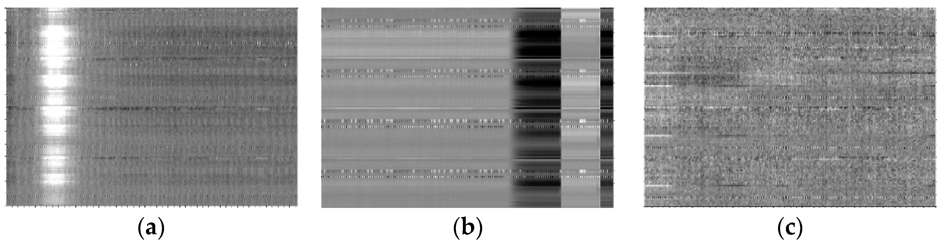
2. Solar Radio Spectrum Dataset and Its Preprocessing
3. Method Section
3.1. Self-Supervised Learning
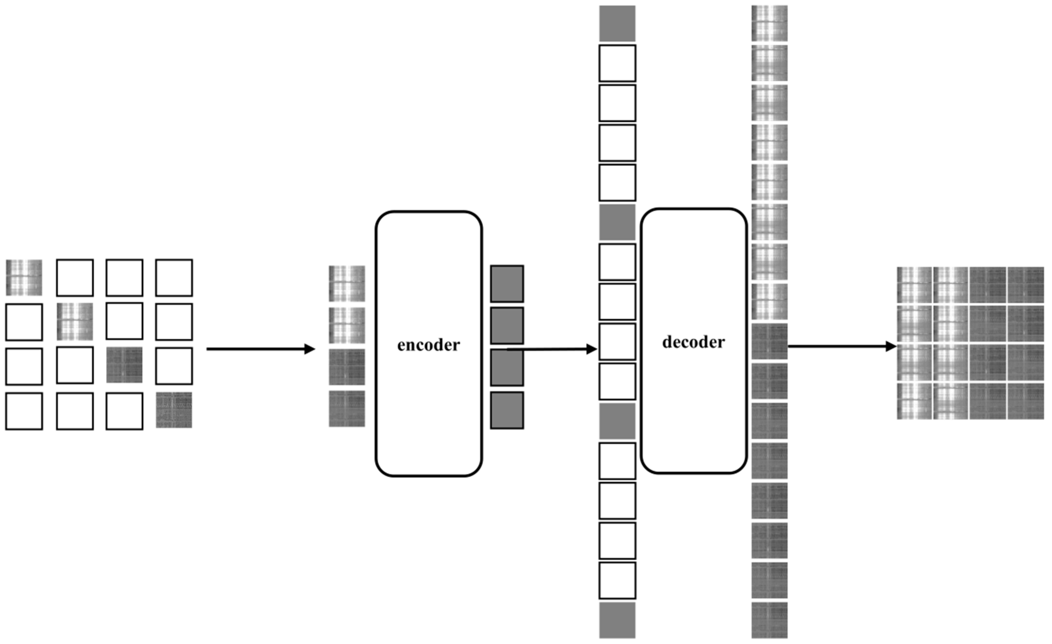
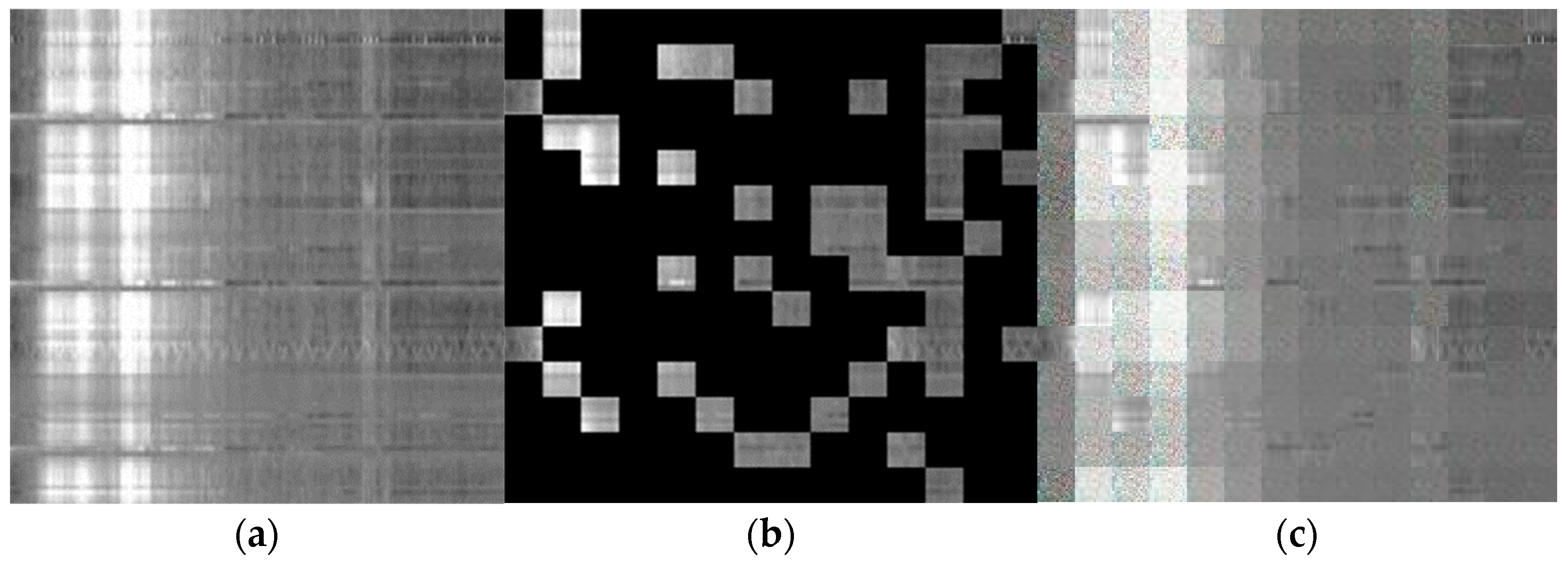
3.2. Self-Supervised Learning with Self-Masking
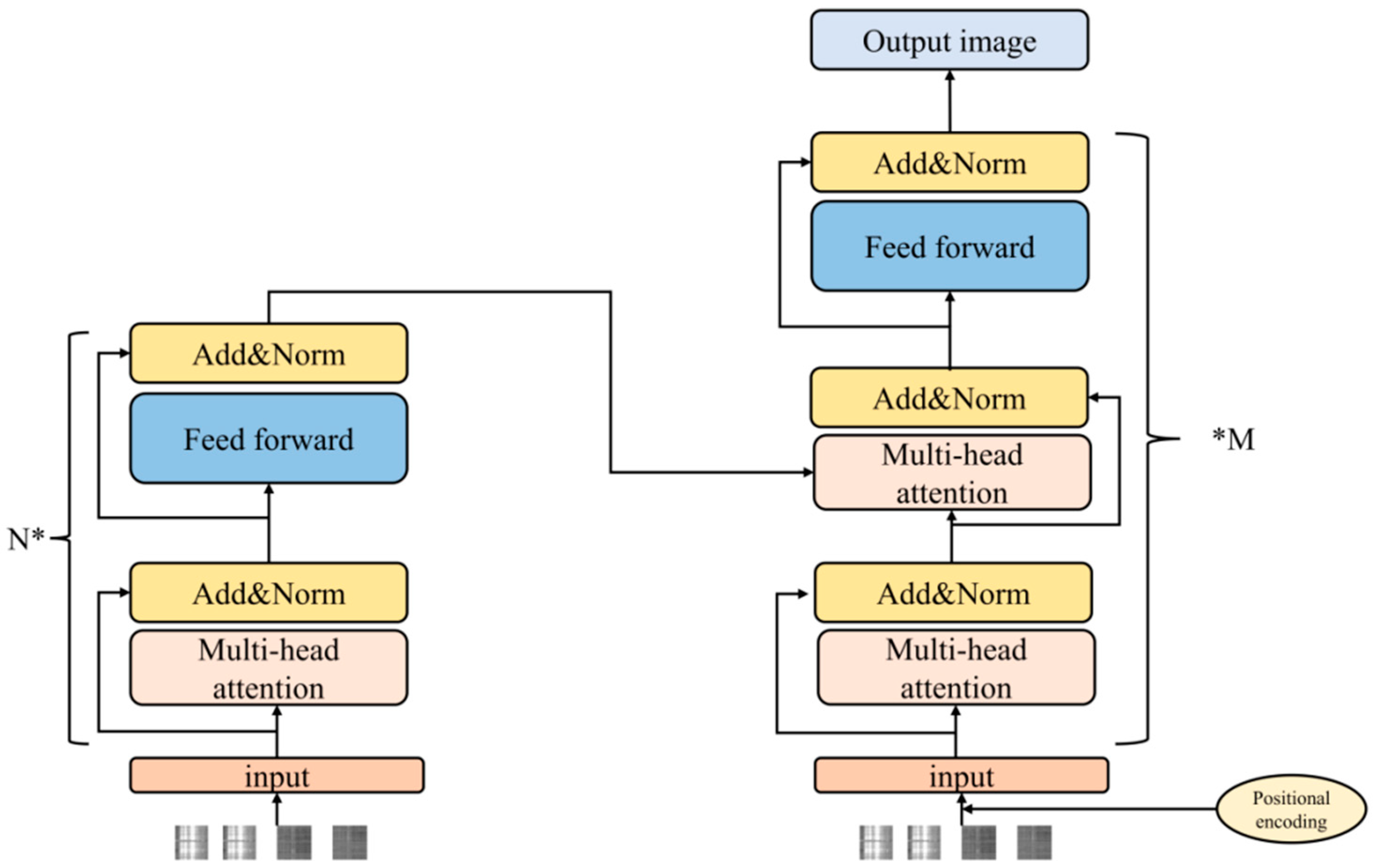
3.3. Encoder and Decoder
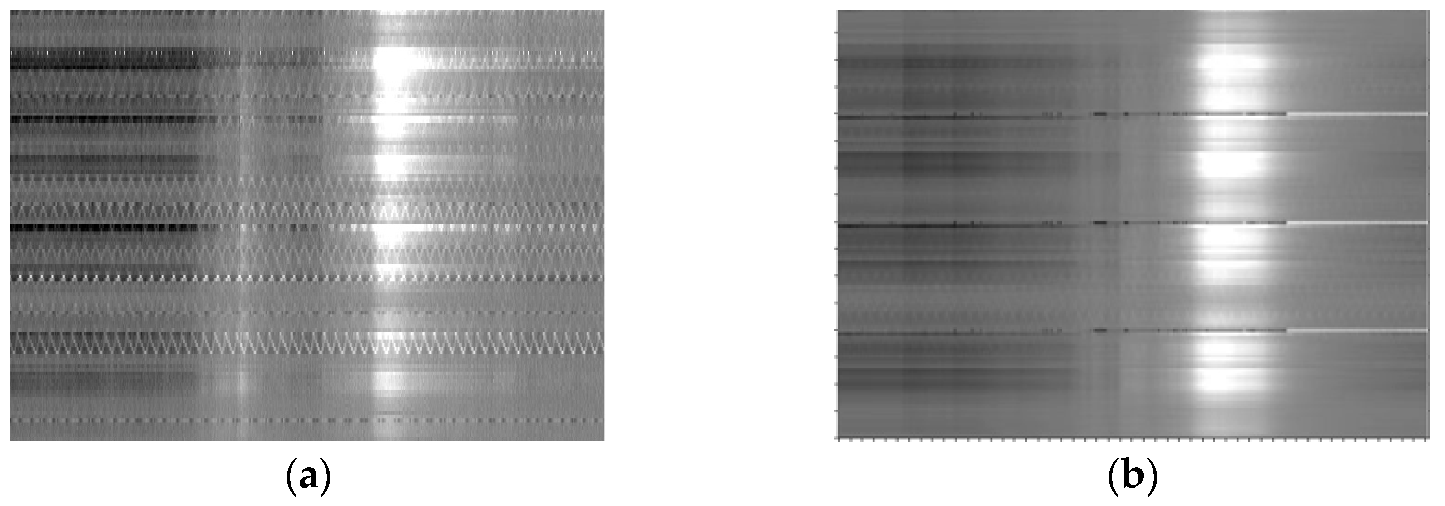
3.4. Data Enhancement
4. Experimental Dataset and Experimental Configuration
4.1. Experimental Dataset
4.2. Experimental Configuration and Evaluation Index
5. Experimental Results and Discussion
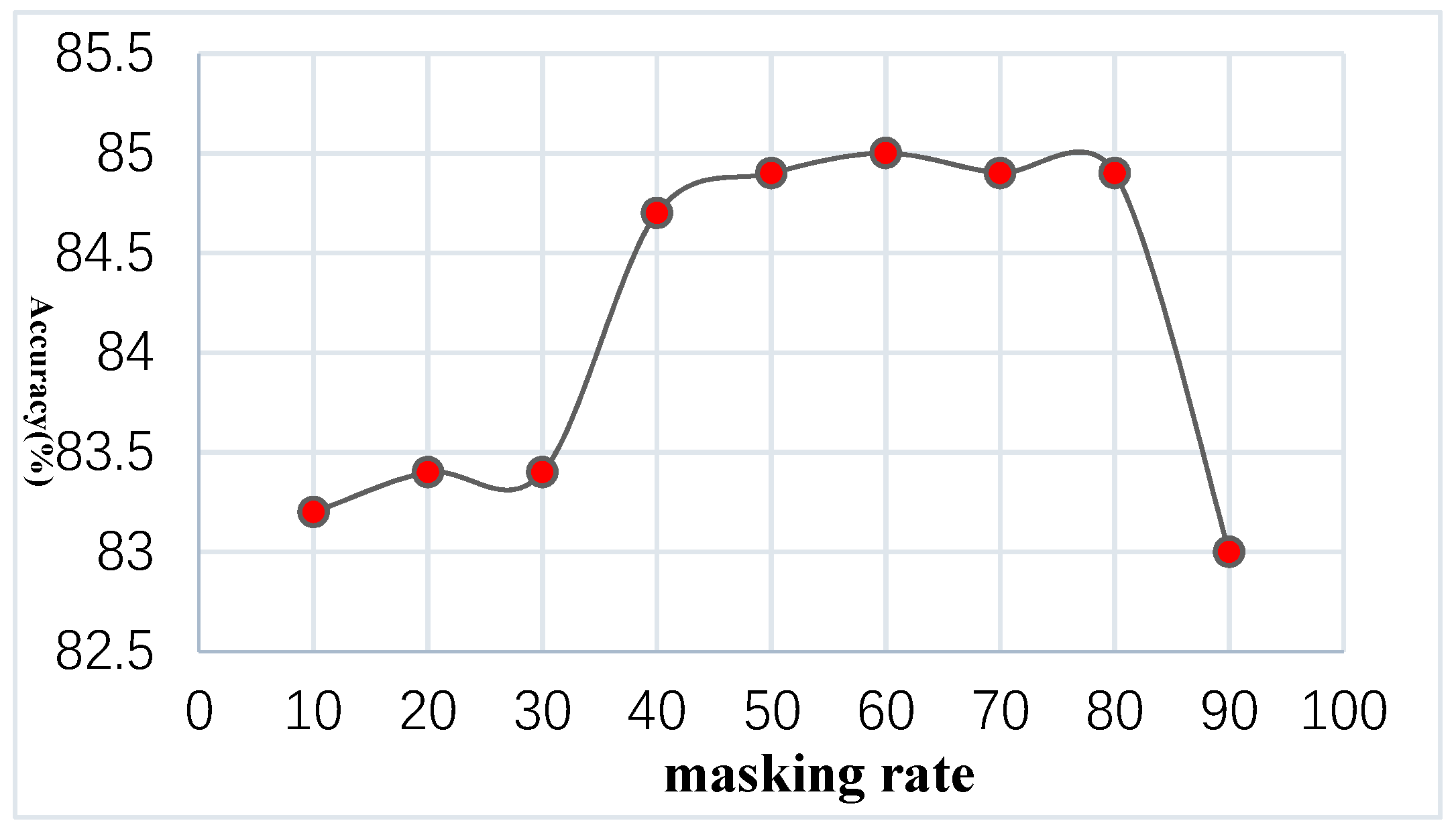
5.1. Effect of Masking Rate on Classification Accuracy
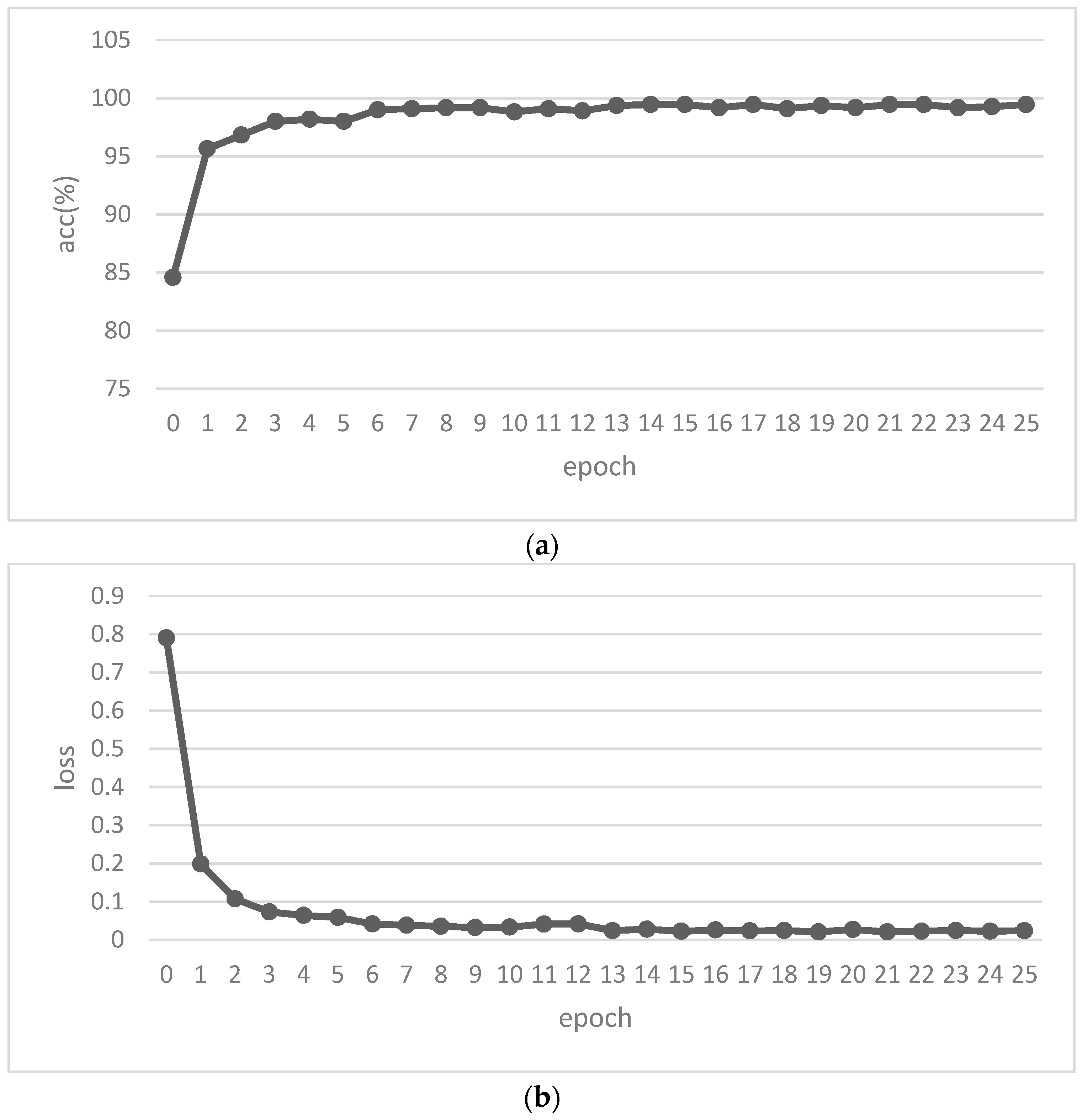
5.2. Pre-Training with Transfer Learning
5.3. Data Enhancement in Training
5.4. Dropout
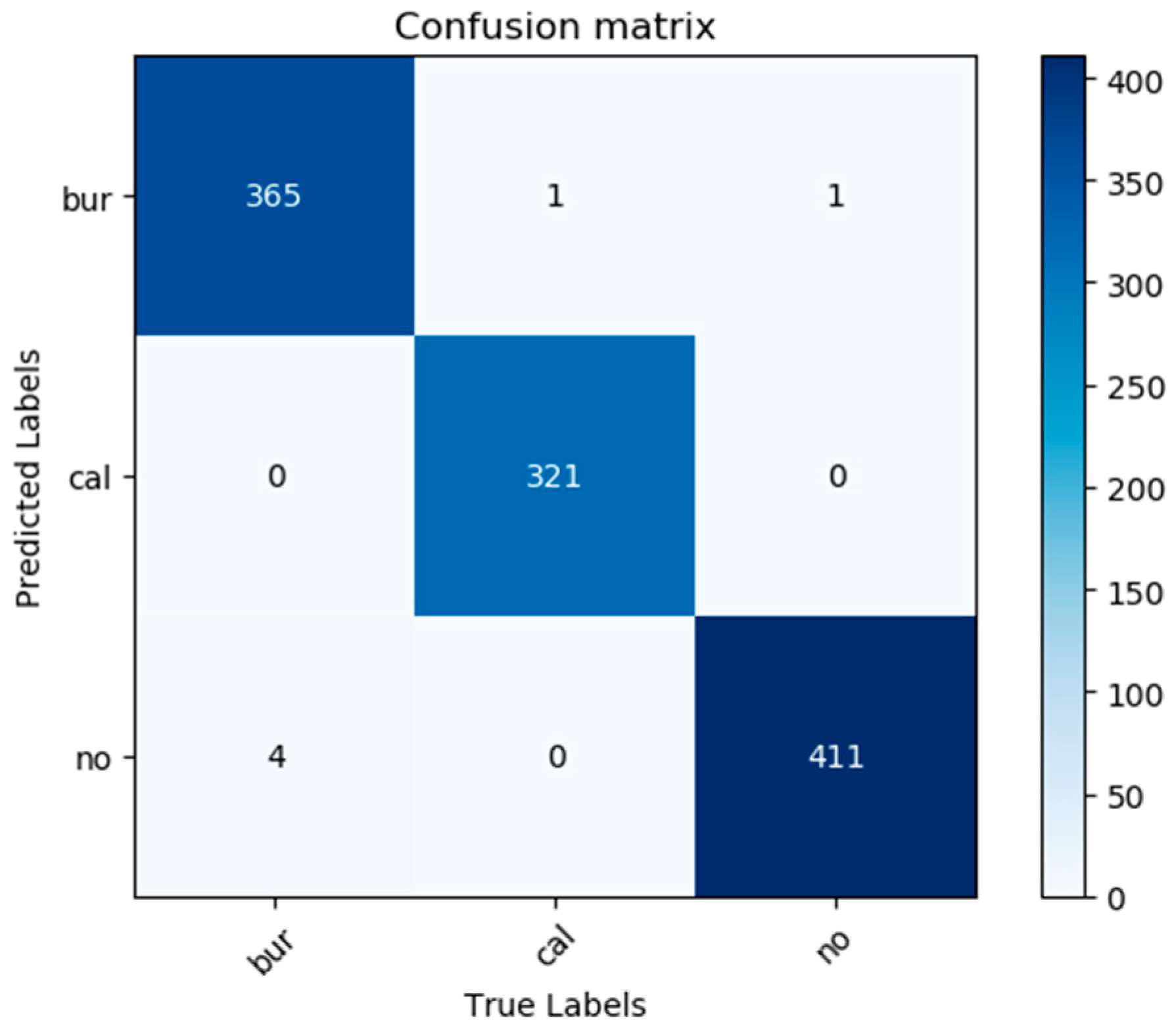
5.5. Final Classification Results
6. Conclusions
Author Contributions
Funding
Data Availability Statement
Acknowledgments
Conflicts of Interest
References
- Singh, D.; Raja, K.S.; Subramanian, P.; Ramesh, R.; Monstein, C. Automated Detection of Solar Radio Bursts Using a Statistical Method. Sol. Phys. 2019, 294, 1500. [Google Scholar] [CrossRef]
- Du, Q.-F. A solar radio dynamic spectrograph with flexible temporal-spectral resolution. Res. Astron. Astrophys. 2017, 17, 98. [Google Scholar] [CrossRef][Green Version]
- Liu, Y.; Ren, D.; Yan, F.; Wu, Z.; Dong, Z.; Chen, Y. Performance comparison of power divider and fiber splitter in the fiber-based frequency transmission system of solar radio observation. IEEE Access 2021, 9, 24925–24932. [Google Scholar] [CrossRef]
- Fu, Q. A new solar broadband radio spectrometer (SBRS) in China. Sol. Phys. 2004, 222, 167–173. [Google Scholar] [CrossRef]
- Ma, L.; Chen, Z.; Xu, L.; Yan, Y. Multimodal deep learning for solar radio burst classification. Pattern Recognit. 2017, 61, 573–582. [Google Scholar] [CrossRef]
- Devlin, J.; Chang, M.W.; Lee, K.; Toutanova, K. BERT: Pre-Training of Deep Bidirectional Transformers for Language Understanding; NAACL HLT: Minneapolis, MN, USA, 2019. [Google Scholar]
- Liu, H.; Yuan, G.; Yang, L.; Liu, K.; Zhou, H. An Appearance Defect Detection Method for Cigarettes Based on C-CenterNet. Electronics 2022, 11, 2182. [Google Scholar] [CrossRef]
- Yang, L.; Yuan, G.; Zhou, H.; Liu, H.; Chen, J.; Wu, H. RS-YOLOX: A High-Precision Detector for Object Detection in Satellite Remote Sensing Images. Appl. Sci. 2022, 12, 8707. [Google Scholar] [CrossRef]
- Yan, F.-B. A broadband digital receiving system with large dynamic range for solar radio observation. Res. Astron. Astrophys. 2020, 20, 156. [Google Scholar] [CrossRef]
- Zhang, P.J.; Wang, C.B.; Ye, L. A type III radio burst automatic analysis system and statistic results for a half solar cycle with Nancay Decameter Array data. Astron. Astrophys. 2018, 618, 33260. [Google Scholar] [CrossRef]
- Krizhevsky, A.; Sutskever, I.; Hinton, G.E. ImageNet classification with deep convolutional neural networks. Commun. ACM. 2017, 60, 84–90. [Google Scholar] [CrossRef]
- Szegedy, C. Going deeper with convolutions. In Proceedings of the 2015 IEEE Conference on Computer Vision and Pattern Recognition (CVPR), Boston, MA, USA, 7–12 June 2015. [Google Scholar]
- Graves, A. Long short-term memory. In Supervised Sequence Labelling with Recurrent Neural Networks; Springer: Berlin/Heidelberg, Germany, 2012; pp. 37–45. [Google Scholar]
- Bengio, Y. Learning deep architectures for AI. Found. Trends® Mach. Learn. 2009, 2, 1–127. [Google Scholar] [CrossRef]
- Chen, S.S. Research on Classification Algorithm of Solar Radio Spectrum Based on Convolutional Neural Network. Master’s Thesis, Shenzhen University, Shenzhen, China, 2018. [Google Scholar]
- Jalali, S.M.J.; Ahmadian, S.; Kavousi-Fard, A.; Khosravi, A.; Nahavandi, S. Automated deep CNN-LSTM architecture design for solar irradiance forecasting. IEEE Trans. Syst. Man. 2021, 52, 54–65. [Google Scholar] [CrossRef]
- Yan, B.; Wang, X.; Hu, C.; Wu, D.; Xia, J. Asymmetrical and symmetrical naphthalene monoimide fused perylene diimide acceptors for organic solar cells. Tetrahedron 2022, 116, 132818. [Google Scholar] [CrossRef]
- He, K.; Zhang, X.; Ren, S.; Sun, J. Deep residual learning for image recognition. In Proceedings of the 2016 IEEE Conference on Computer Vision and Pattern Recognition (CVPR), Las Vegas, NV, USA, 27–30 June 2016. [Google Scholar]
- Salmane, H.; Weber, R.; Abed-Meraim, K.; Klein, K.-L.; Bonnin, X. A method for the automated detection of solar radio bursts in dynamic spectra. J. Space Weather. Space Clim. 2018, 8, A43. [Google Scholar] [CrossRef]
- Vaswani, A. Attention is All You Need; NIPS: Long Beach, LA, USA, 2017. [Google Scholar]
- Han, K. A survey on visual transformer. arXiv 2020, arXiv:2012.12556. [Google Scholar]
- Bhunia, A.K.; Chowdhury, P.N.; Yang, Y.; Hospedales, T.M.; Xiang, T.; Song, Y.-Z. Vectorization and rasterization: Self-supervised learning for sketch and handwriting. In Proceedings of the 2021 IEEE/CVF Conference on Computer Vision and Pattern Recognition (CVPR), Nashville, TN, USA, 20–25 June 2021. [Google Scholar]
- Yue, X. Prototypical cross-domain self-supervised learning for few-shot unsupervised domain adaptation. In Proceedings of the 2021 IEEE/CVF Conference on Computer Vision and Pattern Recognition (CVPR), Nashville, TN, USA, 20–25 June 2021. [Google Scholar]
- Yang, J.; Alvarez, J.M.; Liu, M. Self-supervised learning of depth inference for multi-view stereo. In Proceedings of the 2021 IEEE/CVF Conference on Computer Vision and Pattern Recognition (CVPR), Nashville, TN, USA, 20–25 June 2021. [Google Scholar]
- Reed, C.J.; Metzger, S.; Darrell, T.S.; Keutzer, K. Selfaugment: Automatic augmentation policies for self-supervised learning. In Proceedings of the 2021 IEEE/CVF Conference on Computer Vision and Pattern Recognition (CVPR), Nashville, TN, USA, 20–25 June 2021. [Google Scholar]
- Dosovitskiy, A. An image is worth 16 × 16 words: Transformers for image recognition at scale. arXiv 2020, arXiv:2010.11929. [Google Scholar]
- Liu, Z. Swin Transformer: Hierarchical Vision Transformer using Shifted Windows. In Proceedings of the 2021 IEEE/CVF International Conference on Computer Vision Workshops (ICCVW), Montreal, BC, Canada, 11–17 October 2021. [Google Scholar]
- Yuan, L. Tokens-to-Token ViT: Training Vision Transformers from Scratch on ImageNet. In Proceedings of the 2021 IEEE/CVF International Conference on Computer Vision Workshops (ICCVW), Montreal, BC, Canada, 11–17 October 2021. [Google Scholar]
- Wang, W. Pyramid Vision Transformer: A Versatile Backbone for Dense Prediction without Convolutions. In Proceedings of the 2021 IEEE/CVF International Conference on Computer Vision Workshops (ICCVW), Montreal, BC, Canada, 11–17 October 2021. [Google Scholar]
- Zhu, X.; Su, W.; Lu, L.; Li, B.; Wang, X.; Dai, J. Deformable DETR: Deformable Transformers for End-to-End Object Detection. arXiv 2020, arXiv:2010.04159. [Google Scholar]
- Deng, J.; Dong, W.; Socher, R. Imagenet: A large-scale hierarchical image database. In Proceedings of the 2009 IEEE Conference on Computer Vision and Pattern Recognition, Miami, FL, USA, 20–25 June 2009. [Google Scholar]
- Zehui, L.; Liu, P.; Huang, L. DropAttention: A Regularization Method for Fully-Connected Self-Attention Networks. arXiv 2019, arXiv:1907.11065. [Google Scholar]


| Type | Training Set | Testing Set | Total |
|---|---|---|---|
| Non-burst | 1648 | 412 | 2060 |
| Burst | 1476 | 369 | 1845 |
| Calibration | 1292 | 322 | 1614 |
| Method | Accuracy (%) |
|---|---|
| Training from the beginning | 70.60 |
| Transfer learning | 98.63 |
| Mixing Method | Accuracy (%) | Recall (%) | ||
|---|---|---|---|---|
| Random Erasing | 96.7 | 97.8 | ||
| Color change | 98.6 | 98.4 | ||
| Mixup | +Quadratic interpolation | +Random | 98.7 | 97.3 |
| +Triple interpolation | +Batch | 98.1 | 97.8 | |
| +Quadratic interpolation | +Batch | 98.7 | 98.4 | |
| +Triple interpolation | +Random | 98.9 | 97.6 | |
| Cutmix | +Batch | 98.8 | 97.0 | |
| +Random | 98.7 | 97.3 | ||
| Mixup + Cutmix | 99.3 | 98.4 | ||
| Method | Accuracy (%) | Recall (%) |
|---|---|---|
| Dropout | 98.8 | 97.8 |
| DropPath | 98.9 | 98.4 |
| DropAttention | 98.6 | 98.4 |
| Type | Precision (%) | Recall (%) | Specificity (%) | F1 Score |
|---|---|---|---|---|
| Burst | 99.5 | 98.9 | 99.7 | 0.992 |
| Non-burst | 99.0 | 99.8 | 99.4 | 0.994 |
| Calibration | 100 | 99.7 | 100 | 0.998 |
| Models | Accuracy (%) | Recall (%) |
|---|---|---|
| Vision Transformer | 94.3 | 97.5 |
| VGG16 | 96.0 | 98.4 |
| Swin Transformer | 99.0 | 99.1 |
| Resnet | 98.9 | 98.9 |
| MobileNet | 95.6 | 98.1 |
| GoogLeNet | 96.6 | 98.4 |
| DenseNet | 99.1 | 99.1 |
| Ours | 99.5 | 99.7 |
Publisher’s Note: MDPI stays neutral with regard to jurisdictional claims in published maps and institutional affiliations. |
© 2022 by the authors. Licensee MDPI, Basel, Switzerland. This article is an open access article distributed under the terms and conditions of the Creative Commons Attribution (CC BY) license (https://creativecommons.org/licenses/by/4.0/).
Share and Cite
Li, S.; Yuan, G.; Chen, J.; Tan, C.; Zhou, H. Self-Supervised Learning for Solar Radio Spectrum Classification. Universe 2022, 8, 656. https://doi.org/10.3390/universe8120656
Li S, Yuan G, Chen J, Tan C, Zhou H. Self-Supervised Learning for Solar Radio Spectrum Classification. Universe. 2022; 8(12):656. https://doi.org/10.3390/universe8120656
Chicago/Turabian StyleLi, Siqi, Guowu Yuan, Jian Chen, Chengming Tan, and Hao Zhou. 2022. "Self-Supervised Learning for Solar Radio Spectrum Classification" Universe 8, no. 12: 656. https://doi.org/10.3390/universe8120656
APA StyleLi, S., Yuan, G., Chen, J., Tan, C., & Zhou, H. (2022). Self-Supervised Learning for Solar Radio Spectrum Classification. Universe, 8(12), 656. https://doi.org/10.3390/universe8120656