Nonsingular Phantom Cosmology in Five-Dimensional f(R, T) Gravity

Abstract

We obtain exact solutions to the field equations for five-dimensional locally rotationally symmetric (LRS) Bianchi type-I spacetime in the $f(R,T)$ theory of gravity, where specifically, the following three cases are considered: (i) $f(R,T)=\mu (R+T)$, (ii) $f(R,T)=R\mu +RT{\mu }^2$, and (iii) $f(R,T)=R+\mu R^2+\mu T$, where R and T, respectively, are the Ricci scalar and trace of the energy–momentum tensor. It is found that the equation of state (EOS) parameter w is governed by the parameter $\mu$ involved in the $f(R,T)$ expressions. We fine-tune the parameter $\mu$ to obtain the effect of phantom energy in the model. However, we also restrict this parameter to obtain a stable model of the universe.

1. Introduction

Researchers have found it impossible to prevent the addition of dimensions and the unification of forces in nature. It is notable that space and time can be seen as a combined fourth component of special relativity, according to Minkowski [1,2]. In a similar way, Maxwell combined the theories of electricity and magnetism. The next step in this regard was to combine electromagnetism with general relativity (GR) [3]. Over the years, many researchers have been trying to construct unified field theories that geometrize all the fundamental forces of nature. The geometrization of gravity by the general theory of relativity (GR) motivated scientists to propose a higher-dimensional theory that can unify gravitation and electromagnetism [4,5]. Essentially, it has been considered that gravity and electromagnetism are coupled via an additional dimension in the higher-dimensional models in general relativity.

In their interesting work, Chodos and Detweiler [6] showed the evolution of a $5d$ vacuum universe into a cogent four-dimensional one. Alvarez and Gavela [7] discussed the cosmological scenario in which the dynamical compactification of the higher dimensions produces an abundance of entropy in the universe. Further, they pointed out the possibility of solving the flatness and horizon problems in this scenario.

Using the Kaluza–Klein (KK) theory [4,5], later on, Marciano [8] investigated the mechanism of the evolution of the fundamental constants throughout cosmic time. For this purpose, he derived unique relationships between the low-energy couplings, as well as the masses and propounded that a time variation in any of these parameters can render the proof of higher dimensions. He also reviewed available experimental bounds and, therefore, urged the requirement of new measurements. On the other hand, Gegenberg and Das [9] constructed $5d$ cosmological models with a real massless non-self interacting scalar field source and pointed out that non-trivial solutions to the field equations occur only when the homogeneous and isotropic three-space has non-positive constant curvature. It is also interesting to note that Lorenz-Petzold [10] obtained exact solutions to the higher-dimensional field equations in a vacuum, as well as the perfect fluid case along with a non-vanishing cosmological constant.

Wesson [11] considered the higher-dimensional spacetimes with a new challenge by pointing out that “the space part of its metric varies with time in the same way as the de Sitter solution of the conventional four-dimensional theory” and formulated his so-called five-dimensional gravitational theory. Under this theory, Grøn [12] successfully obtained vacuum, radiation, and matter-dominated cosmological models. These models describe an inflationary universe in the variable rest-mass theory as was proposed by Wesson (vide the proposition and application of five-dimensional cosmological principle by Wesson in the Book [13]).

Several authors [14,15,16] have discussed the KK extension of the FRW cosmological models. In higher dimensions, anisotropic generalizations of these models are available in the literature [17,18,19], whereas inhomogeneous cosmologies in $5d$ have been studied by other authors [20,21,22]. A few exact solutions to the Einstein field equations in KK spacetime were obtained by various authors and showed that those reproduce, as well as extend the known solutions of the four dimensions [23,24,25]. The exact solution to the Einstein field equations, which is Ricci and Riemannian flat in $5d$, was obtained by Liko and Wesson [26]. Interestingly, this solution in 4d represents a cosmological model for the early vacuum-dominated universe. Some noteworthy works where variable G and $\Lambda$ have been studied [27,28] have immense consequences in KK cosmology and higher-dimensional geometry, e.g., Pahwa [29] constructed a homogeneous, anisotropic $4+d$ cosmological model and, hence, studied the late-time acceleration of the universe.

Higher-dimensional cosmology in various alternative theories of gravity can also be found in the literature, which originated due to a few drawbacks of Einstein’s general relativity (specifically, GR has failed to explain the late-time cosmic acceleration phenomena) and, hence, to comply with the observational evidence. Therefore, one possible technique to justify the observational data [30,31,32,33,34,35,36,37] is the modification of GR. Harko et al. [38] obtained the gravitational field equations in the metric formalism and the equations of motion for the test particles. This theory is called the $f(R,T)$ theory of gravity, where the Lagrangian is an arbitrary function of R and T being the Ricci scalar and trace of the energy–momentum, respectively. Under $f(R,T)$ gravity, various authors have studied different mathematical aspects, as well as physical applications of the theory [39,40,41,42,43,44,45,46,47,48,49,50,51,52,53,54,55,56,57,58,59,60,61,62,63].

We design the present article as follows: We provide the basic equations, as well as the Einstein field equations under the cosmological system in Section 2. In Section 3, we have the exact solutions sets under three specific cases, whereas in Section 4, the behavior of the models is presented and analyzed. The results and their discussion are presented in Section 5 to provide some concluding remarks along with salient features. In the current work, units are expressed using the natural system with $G=c=\hslash =1$.

2. Modified Einstein Field Equations

In their theory, Harko et al. [38] considered three explicit functional forms of $f(R,T)$, which is an arbitrary function of the Ricci scalar R and of the trace of the stress–energy tensor T, as follows:

$$\begin{array}{c}\hfill f(R,T)=\left\{\begin{array}{c}R+2f\left(T\right),\hfill \\ f_1\left(R\right)+f_2\left(T\right),\hfill \\ f_1\left(R\right)+f_2\left(R\right)f_3\left(T\right).\hfill \end{array}\right.\end{array}$$

(1)

One can therefore obtain several theoretical models for each choice of $f(R,T)$. However, in the present work, we consider the second and third case, i.e., $f(R,T)=f_1\left(R\right)+f_2\left(T\right)$ and $f(R,T)=f_1\left(R\right)+f_2\left(R\right)f_3\left(T\right)$, for constructing cosmological models through the $5d$ locally rotationally symmetric (LRS) Bianchi type-I spacetime metric in the form

$$d{s}^2=d{t}^2-A{\left(t\right)}^{2}d{x}^2-B{\left(t\right)}^2(d{y}^2+d{z}^2)-F{\left(t\right)}^{2}d{n}^2,$$

(2)

where A, B, and F are functions of the time coordinate only and the extra dimension n is the space like coordinate.

Now, the gravitational field equations can be provided as [38]

$$\begin{array}{c}\hfill f_R(R,T)R_{ij}-\frac{1}{2}{g}_{ij}f(R,T)+(g_{ij}\square -{\nabla }_i{\nabla }_j)f_R(R,T)=\\ \hfill 8\pi T_{ij}-f_T(R,T)T_{ij}-f_T(R,T){\mathsf{\Theta }}_{ij},\end{array}$$

(3)

where $f_R(R,T)=\frac{\partial f(R,T)}{\partial R}$ and $f_T(R,T)=\frac{\partial f(R,T)}{\partial T}$ are the partial derivative with respect to R and T, respectively, $\square ={\nabla }_i{\nabla }^i$, ${\nabla }_i$ denotes covariant derivatives, and ${\mathsf{\Theta }}_{ij}=-2T_{ij}-g_{ij}P$.

Various authors have studied the choice of Lagrangian density for matter, i.e., ${\mathcal{L}}_m=P$ [64,65,66], and have addressed the problem of Lagrangian density for perfect fluids where P is the pressure. In this case, we assume that the entire universe is filled with a perfect fluid. The choice for the matter Lagrangian density is thus made to be ${\mathcal{L}}_m=-P$ [67].

Here, we consider the source of gravitation as the perfect fluid. Therefore, the energy–momentum tensor is taken as

$$\begin{array}{c}\hfill T_{ij}=(P+\rho )u_i{u}_j-P{g}_{ij},\end{array}$$

(4)

together with the comoving coordinates

$$\begin{array}{c}\hfill g_{ij}{u}^i{u}^j=1.\end{array}$$

(5)

In the above equations, $\rho$ and $u_i$ are the energy density and five-velocity vector of the cosmic fluid distribution, respectively.

3. Solutions to the Field Equations

3.1. $f(R,T)=\mu R+\mu T$

Let us consider here the second case, i.e., $f(R,T)=f_1\left(R\right)+f_2\left(T\right)$ with $f_1\left(R\right)=\mu R$, $f_2\left(T\right)=\mu T$, where

$$R=\frac{2A_{tt}}{A}+\frac{4A_t{B}_t}{AB}+\frac{2A_t{F}_t}{AF}+\frac{4B_{tt}}{B}+\frac{4B_t{F}_t}{BF}+\frac{2B_t^2}{B^2}+\frac{2F_{tt}}{F},$$

$T=\rho \left(t\right)-4P\left(t\right)$, and $\mu$ is an arbitrary constant.

Now, Equation (3) becomes

$$\begin{array}{c}\hfill G_{ij}=\left[\frac{8\pi +\mu }{\mu }\right]T_{ij}+\left[P+\frac{T}{2}\right]g_{ij}.\end{array}$$

(6)

Here, $G_{ij}=R_{ij}-\frac{1}{2}{g}_{ij}R$ is the Einstein tensor. For the line element (2), the explicit form of the field Equation (6) using (4) and (5) can be obtained as

$$-\frac{2\mu A_t{B}_t}{AB}-\frac{\mu A_t{F}_t}{AF}-\frac{2\mu B_t{F}_t}{BF}-\frac{\mu B_t^2}{B^2}+\mu P-\frac{3}{2}\mu \rho -8\pi \rho =0,$$

(7)

$$\frac{2\mu B_{tt}}{B}+\frac{2\mu B_t{F}_t}{BF}+\frac{\mu B_t^2}{B^2}+\frac{\mu F_{tt}}{F}-2\mu P-8\pi P+\frac{1}{2}\mu \rho =0,$$

(8)

$$\frac{\mu A_{tt}}{A}+\frac{\mu A_t{B}_t}{AB}+\frac{\mu A_t{F}_t}{AF}+\frac{\mu B_{tt}}{B}+\frac{\mu B_t{F}_t}{BF}+\frac{\mu F_{tt}}{F}-2\mu P-8\pi P+\frac{1}{2}\mu \rho =0,$$

(9)

$$\frac{\mu A_{tt}}{A}+\frac{2\mu A_t{B}_t}{AB}+\frac{2\mu B_{tt}}{B}+\frac{\mu B_t^2}{B^2}-2\mu P-8\pi P+\frac{1}{2}\mu \rho =0.$$

(10)

Here and in what follows, the suffix $“t”$ after a field variable represents an ordinary differentiation with respect to the time $“t”$.

In order to derive the exact solution of the field Equations (7)–(10), we take the following scale transformations [68]:

$$\begin{array}{ccc}\hfill A\left(t\right)& =& e^{\alpha \left(\tau \right)},\hfill \\ \hfill B\left(t\right)& =& e^{\gamma \left(\tau \right)},\hfill \\ \hfill F\left(t\right)& =& e^{\lambda \left(\tau \right)}\hfill \\ \hfill dt& =& A{B}^{2}Fd\tau .\hfill \end{array}$$

(11)

Now, the field Equations (7)–(10) using (11) reduce to

$$2\mu P-(3\mu +16\pi )\rho +e^{-2(\alpha +2\gamma +\lambda )}[-2\mu {\lambda }^{{}^{\prime }}({\alpha }^{{}^{\prime }}+2{\gamma }^{{}^{\prime }})-2\mu {\gamma }^{{}^{\prime }}(2{\alpha }^{{}^{\prime }}+{\gamma }^{{}^{\prime }})]=0$$

(12)

$$\mu (\rho -2e^{-2(\alpha +2\gamma +\lambda )}[{\lambda }^{{}^{\prime }}({\alpha }^{{}^{\prime }}+2{\gamma }^{{}^{\prime }})+{\gamma }^{{}^{\prime }}(2{\alpha }^{{}^{\prime }}+{\gamma }^{{}^{\prime }})-2{\gamma }^{{}^{″}}-{\lambda }^{{}^{″}})]-4(\mu +4\pi )P=0$$

(13)

$$e^{2(\alpha +2\gamma +\lambda )}[\mu \rho -4(\mu +4\pi )P]+2\mu [{\alpha }^{{}^{″}}-{\alpha }^{{}^{\prime }}(2{\gamma }^{{}^{\prime }}+{\lambda }^{{}^{\prime }})+{\gamma }^{{}^{″}}-{\gamma }^{{}^{\prime }}({\gamma }^{{}^{\prime }}+2{\lambda }^{{}^{\prime }})+{\lambda }^{{}^{″}}]=0,$$

(14)

$$\mu (\rho -2e^{-2(\alpha +2\gamma +\lambda )}[-{\alpha }^{{}^{″}}+{\lambda }^{{}^{\prime }}({\alpha }^{{}^{\prime }}+2{\gamma }^{{}^{\prime }})+{\gamma }^{{}^{\prime }}(2{\alpha }^{{}^{\prime }}+{\gamma }^{{}^{\prime }})-2{\gamma }^{{}^{″}})]-4(\mu +4\pi )P=0,$$

(15)

where the prime stands for $\frac{d}{d\tau }$.

It is to be noted that there are five unknowns $\alpha$, $\gamma$, $\lambda$, P, and $\rho$ involved in the above four equations. Therefore, for obtaining exact solutions of Equations (12)–(15), we need to consider some interplaying relationships between any two parameters, such as [69,70,71]

$$\begin{array}{c}\hfill \lambda =m\gamma ,\end{array}$$

(16)

where $m\ne 0$ is a parameter, the value of which can be chosen suitably depending on the physical situation.

Now, solving Equations (12)–(15), we obtain the solutions as

$$\begin{array}{c}\hfill \gamma \left(\tau \right)=k_1\tau +k_2,\end{array}$$

(17)

$$\begin{array}{c}\hfill \lambda \left(\tau \right)=m(k_1\tau +k_2),\end{array}$$

(18)

$$\begin{array}{c}\hfill \alpha \left(\tau \right)=k_3\tau +k_4,\end{array}$$

(19)

$$\begin{array}{c}\hfill \rho =-\frac{2\mu (3\mu +8\pi )\left(c_1{e}^{-2\tau c_2}\right)}{(\mu +8\pi )(5\mu +16\pi )},\end{array}$$

(20)

$$\begin{array}{c}\hfill P=-\frac{4\mu (\mu +4\pi )\left(c_1{e}^{-2\tau c_2}\right)}{(\mu +8\pi )(5\mu +16\pi )},\end{array}$$

(21)

where $k_1$, $k_2$, $k_3$, and $k_4$ are the integration constant and $c_1=k_1[2k_{1}m+k_1+k_3(m+2)]$ and $c_2=k_1(m+2)+k_3$. Without loss of generality, we take $k_2=k_4=0$.

3.2. $f(R,T)=R+\mu R^2+\mu T$

In this case, we consider $f_1\left(R\right)=R+\mu R^2$ and $f_2\left(T\right)=\mu T$. Therefore, Equation (3) becomes

$$G_{ij}+2\mu R{R}_{ij}-\frac{1}{2}\mu R^2{g}_{ij}+2\mu (g_{ij}\square -{\nabla }_i{\nabla }_j)R=(8\pi +\mu )T_{ij}+\left(P+\frac{T}{2}\right)\mu g_{ij}.$$

(22)

For (2), the field equations in $f(R,T)$ theory using (11) and (22) become

$$\begin{array}{c}\hfill -2{\left({\gamma }^{{}^{\prime }}\right)}^2(8\mu (7{\alpha }^{{}^{″}}+12{\gamma }^{{}^{″}}+7{\lambda }^{{}^{″}}-12{\left({\lambda }^{{}^{\prime }}\right)}^2)+e^{2(\alpha +2\gamma +\lambda )})+\\ \hfill 16\mu {\left({\alpha }^{{}^{\prime }}\right)}^3(2{\gamma }^{{}^{\prime }}+{\lambda }^{{}^{\prime }})+4\mu (2{\lambda }^{{}^{\prime }}({\alpha }^{\left(3\right)}+2{\gamma }^{\left(3\right)}+{\lambda }^{\left(3\right)})+{({\alpha }^{{}^{″}}+2{\gamma }^{{}^{″}}+{\lambda }^{{}^{″}})}^2-\\ \hfill 2{\left({\lambda }^{{}^{\prime }}\right)}^2(3{\alpha }^{{}^{″}}+6{\gamma }^{{}^{″}}+2{\lambda }^{{}^{″}}))+4{\gamma }^{{}^{\prime }}(4\mu ({\alpha }^{\left(3\right)}+2{\gamma }^{\left(3\right)}+{\lambda }^{\left(3\right)})-\\ \hfill {\lambda }^{{}^{\prime }}(4\mu (8{\alpha }^{{}^{″}}+15{\gamma }^{{}^{″}}+7{\lambda }^{{}^{″}})+e^{2(\alpha +2\gamma +\lambda )})+8\mu {\left({\lambda }^{{}^{\prime }}\right)}^3)+\\ \hfill 4\mu {\left({\alpha }^{{}^{\prime }}\right)}^2(-2(2{\alpha }^{{}^{″}}+6{\gamma }^{{}^{″}}+3{\lambda }^{{}^{″}})+52{\gamma }^{{}^{\prime }}{\lambda }^{{}^{\prime }}+48{\left({\gamma }^{{}^{\prime }}\right)}^2+11{\left({\lambda }^{{}^{\prime }}\right)}^2)+\\ \hfill 2{\alpha }^{{}^{\prime }}\left(4\mu \right({\alpha }^{\left(3\right)}-{\lambda }^{{}^{\prime }}(7{\alpha }^{{}^{″}}+16{\gamma }^{{}^{″}}+7{\lambda }^{{}^{″}})+\\ \hfill 2{\gamma }^{{}^{\prime }}(-7{\alpha }^{{}^{″}}-15{\gamma }^{{}^{″}}-8{\lambda }^{{}^{″}}+13{\left({\lambda }^{{}^{\prime }}\right)}^2)+2{\gamma }^{\left(3\right)}+59{\left({\gamma }^{{}^{\prime }}\right)}^2{\lambda }^{{}^{\prime }}+\\ \hfill 30{\left({\gamma }^{{}^{\prime }}\right)}^3+{\lambda }^{\left(3\right)}+2{\left({\lambda }^{{}^{\prime }}\right)}^3)-e^{2(\alpha +2\gamma +\lambda )}(2{\gamma }^{{}^{\prime }}+{\lambda }^{{}^{\prime }}))+240\mu {\left({\gamma }^{{}^{\prime }}\right)}^3{\lambda }^{{}^{\prime }}+\\ \hfill 76\mu {\left({\gamma }^{{}^{\prime }}\right)}^4+e^{4(\alpha +2\gamma +\lambda )}(-3\mu \rho +2\mu P-16\rho \pi )=0,\end{array}$$

(23)

$$\begin{array}{c}\hfill -2{\left({\gamma }^{{}^{\prime }}\right)}^2(4\mu (34{\alpha }^{{}^{″}}+54{\gamma }^{{}^{″}}+35{\lambda }^{{}^{″}}-38{\left({\lambda }^{{}^{\prime }}\right)}^2)+e^{2(\alpha +2\gamma +\lambda )})+\\ \hfill 48\mu {\left({\alpha }^{{}^{\prime }}\right)}^3(2{\gamma }^{{}^{\prime }}+{\lambda }^{{}^{\prime }})+4{\gamma }^{{}^{\prime }}(4\mu (5{\alpha }^{\left(3\right)}+9{\gamma }^{\left(3\right)}+5{\lambda }^{\left(3\right)})-\\ \hfill {\lambda }^{{}^{\prime }}(72\mu {\alpha }^{{}^{″}}+e^{2(\alpha +2\gamma +\lambda )}+136\mu {\gamma }^{{}^{″}}+60\mu {\lambda }^{{}^{″}})+16\mu {\left({\lambda }^{{}^{\prime }}\right)}^3)+\\ \hfill 4\mu {\left({\alpha }^{{}^{\prime }}\right)}^2(3(4{\gamma }^{{}^{\prime }}+{\lambda }^{{}^{\prime }})(8{\gamma }^{{}^{\prime }}+7{\lambda }^{{}^{\prime }})-2(6{\alpha }^{{}^{″}}+11(2{\gamma }^{{}^{\prime \prime }}+{\lambda }^{{}^{\prime \prime }})))+\\ \hfill 4\mu (-2({\alpha }^{\left(4\right)}+2{\gamma }^{\left(4\right)}+{\lambda }^{\left(4\right)})+2{\lambda }^{{}^{\prime }}(5{\alpha }^{\left(3\right)}+10{\gamma }^{\left(3\right)}+4{\lambda }^{\left(3\right)})+\\ \hfill 12{\alpha }^{{}^{″}}(2{\gamma }^{{}^{″}}+{\lambda }^{{}^{″}})-8{\left({\lambda }^{{}^{\prime }}\right)}^2(2{\alpha }^{{}^{″}}+4{\gamma }^{{}^{″}}+{\lambda }^{{}^{″}})+3{\left({\alpha }^{{}^{″}}\right)}^2+28{\gamma }^{{}^{″}}{\lambda }^{{}^{″}}+\\ \hfill 24{\left({\gamma }^{{}^{″}}\right)}^2+5{\left({\lambda }^{{}^{″}}\right)}^2)+2{\alpha }^{{}^{\prime }}\left(4\mu \right(5{\alpha }^{\left(3\right)}-{\lambda }^{{}^{\prime }}(17{\alpha }^{{}^{″}}+44{\gamma }^{{}^{″}}+17{\lambda }^{{}^{″}})+\\ \hfill {\gamma }^{{}^{\prime }}(-34{\alpha }^{{}^{″}}-78{\gamma }^{{}^{″}}-44{\lambda }^{{}^{″}}+46{\left({\lambda }^{{}^{\prime }}\right)}^2)+12{\gamma }^{\left(3\right)}+103{\left({\gamma }^{{}^{\prime }}\right)}^2{\lambda }^{{}^{\prime }}+\\ \hfill 54{\left({\gamma }^{{}^{\prime }}\right)}^3+6{\lambda }^{\left(3\right)}+4{\left({\lambda }^{{}^{\prime }}\right)}^3)-e^{2(\alpha +2\gamma +\lambda )}(2{\gamma }^{{}^{\prime }}+{\lambda }^{{}^{\prime }}))2e^{2(\alpha +2\gamma +\lambda )}(2{\gamma }^{{}^{″}}+{\lambda }^{{}^{″}})++\\ \hfill 400\mu {\left({\gamma }^{{}^{\prime }}\right)}^3{\lambda }^{{}^{\prime }}+132\mu {\left({\gamma }^{{}^{\prime }}\right)}^4+e^{4(\alpha +2\gamma +\lambda )}(\mu \rho -4P(\mu +4\pi ))=0,\end{array}$$

(24)

$$\begin{array}{c}\hfill 2e^{2(\alpha +2\gamma +\lambda )}({\alpha }^{{}^{″}}+{\gamma }^{{}^{″}}+{\lambda }^{{}^{″}})-2{\left({\gamma }^{{}^{\prime }}\right)}^2(4\mu (41{\alpha }^{{}^{″}}+63{\gamma }^{{}^{″}}+41{\lambda }^{{}^{″}}-42{\left({\lambda }^{{}^{\prime }}\right)}^2)+\\ \hfill e^{2(\alpha +2\gamma +\lambda )})+32\mu {\left({\alpha }^{{}^{\prime }}\right)}^3(2{\gamma }^{{}^{\prime }}+{\lambda }^{{}^{\prime }})+4{\gamma }^{{}^{\prime }}(2\mu (11{\alpha }^{\left(3\right)}+20{\gamma }^{\left(3\right)}+11{\lambda }^{\left(3\right)})-\\ \hfill {\lambda }^{{}^{\prime }}(82\mu {\alpha }^{{}^{″}}+e^{2(\alpha +2\gamma +\lambda )}+144\mu {\gamma }^{{}^{″}}+64\mu {\lambda }^{{}^{″}})+16\mu {\left({\lambda }^{{}^{\prime }}\right)}^3)+\\ \hfill 4\mu {\left({\alpha }^{{}^{\prime }}\right)}^2(-8({\alpha }^{{}^{″}}+4{\gamma }^{{}^{″}}+2{\lambda }^{{}^{″}})+88{\gamma }^{{}^{\prime }}{\lambda }^{{}^{\prime }}+84{\left({\gamma }^{{}^{\prime }}\right)}^2+17{\left({\lambda }^{{}^{\prime }}\right)}^2)+\\ \hfill 4\mu (-2({\alpha }^{\left(4\right)}+2{\gamma }^{\left(4\right)}+{\lambda }^{\left(4\right)})+2{\lambda }^{{}^{\prime }}(5{\alpha }^{\left(3\right)}+10{\gamma }^{\left(3\right)}+4{\lambda }^{\left(3\right)})+\\ \hfill 2{\alpha }^{{}^{″}}(13{\gamma }^{{}^{″}}+7{\lambda }^{{}^{″}})-8{\left({\lambda }^{{}^{\prime }}\right)}^2(2{\alpha }^{{}^{″}}+4{\gamma }^{{}^{″}}+{\lambda }^{{}^{″}})+5{\left({\alpha }^{{}^{″}}\right)}^2+26{\gamma }^{{}^{″}}{\lambda }^{{}^{″}}+\\ \hfill 20{\left({\gamma }^{{}^{″}}\right)}^2+5{\left({\lambda }^{{}^{″}}\right)}^2)+2{\alpha }^{{}^{\prime }}\left(4\mu \right(4{\alpha }^{\left(3\right)}-{\lambda }^{{}^{\prime }}(15{\alpha }^{{}^{″}}+37{\gamma }^{{}^{″}}+15{\lambda }^{{}^{″}})+\\ \hfill {\gamma }^{{}^{\prime }}(-32{\alpha }^{{}^{″}}-72{\gamma }^{{}^{″}}-41{\lambda }^{{}^{″}}+44{\left({\lambda }^{{}^{\prime }}\right)}^2)+10{\gamma }^{\left(3\right)}+105{\left({\gamma }^{{}^{\prime }}\right)}^2{\lambda }^{{}^{\prime }}+\\ \hfill 60{\left({\gamma }^{{}^{\prime }}\right)}^3+5{\lambda }^{\left(3\right)}+4{\left({\lambda }^{{}^{\prime }}\right)}^3)-e^{2(\alpha +2\gamma +\lambda )}(2{\gamma }^{{}^{\prime }}+{\lambda }^{{}^{\prime }}))+\\ \hfill 480\mu {\left({\gamma }^{{}^{\prime }}\right)}^3{\lambda }^{{}^{\prime }}+164\mu {\left({\gamma }^{{}^{\prime }}\right)}^4+e^{4(\alpha +2\gamma +\lambda )}(\mu \rho -4P(\mu +4\pi ))=0,\end{array}$$

(25)

$$\begin{array}{c}\hfill 2e^{2(\alpha +2\gamma +\lambda )}({\alpha }^{{}^{″}}+2{\gamma }^{{}^{″}})-2{\left({\gamma }^{{}^{\prime }}\right)}^2(4\mu (35{\alpha }^{{}^{″}}+54{\gamma }^{{}^{″}}+34{\lambda }^{{}^{″}}-48{\left({\lambda }^{{}^{\prime }}\right)}^2)+e^{2(\alpha +2\gamma +\lambda )})+\\ \hfill 32\mu {\left({\alpha }^{{}^{\prime }}\right)}^3(2{\gamma }^{{}^{\prime }}+{\lambda }^{{}^{\prime }})+4{\gamma }^{{}^{\prime }}(4\mu (5{\alpha }^{\left(3\right)}+9{\gamma }^{\left(3\right)}+5{\lambda }^{\left(3\right)})-\\ \hfill {\lambda }^{{}^{\prime }}(88\mu {\alpha }^{{}^{″}}+e^{2(\alpha +2\gamma +\lambda )}+156\mu {\gamma }^{{}^{″}}+68\mu {\lambda }^{{}^{″}})+24\mu {\left({\lambda }^{{}^{\prime }}\right)}^3)+\\ \hfill 4\mu {\left({\alpha }^{{}^{\prime }}\right)}^2(-8({\alpha }^{{}^{″}}+4{\gamma }^{{}^{″}}+2{\lambda }^{{}^{″}})+92{\gamma }^{{}^{\prime }}{\lambda }^{{}^{\prime }}+76{\left({\gamma }^{{}^{\prime }}\right)}^2+21{\left({\lambda }^{{}^{\prime }}\right)}^2)+\\ \hfill 4\mu (-2({\alpha }^{\left(4\right)}+2{\gamma }^{\left(4\right)}+{\lambda }^{\left(4\right)})+2{\lambda }^{{}^{\prime }}(6{\alpha }^{\left(3\right)}+12{\gamma }^{\left(3\right)}+5{\lambda }^{\left(3\right)})+\\ \hfill 4{\alpha }^{{}^{″}}(7{\gamma }^{{}^{″}}+3{\lambda }^{{}^{″}})-2{\left({\lambda }^{{}^{\prime }}\right)}^2(11{\alpha }^{{}^{″}}+22{\gamma }^{{}^{″}}+6{\lambda }^{{}^{″}})+\\ \hfill 5{\left({\alpha }^{{}^{″}}\right)}^2+3(8{\gamma }^{{}^{″}}{\lambda }^{{}^{″}}+8{\left({\gamma }^{{}^{\prime \prime }}\right)}^2+{\left({\lambda }^{{}^{\prime \prime }}\right)}^2))+2{\alpha }^{{}^{\prime }}\left(4\mu \right(4{\alpha }^{\left(3\right)}-{\lambda }^{{}^{\prime }}(17{\alpha }^{{}^{″}}+44{\gamma }^{{}^{″}}+17{\lambda }^{{}^{″}})+\\ \hfill {\gamma }^{{}^{\prime }}(-30{\alpha }^{{}^{″}}-68{\gamma }^{{}^{″}}-36{\lambda }^{{}^{″}}+54{\left({\lambda }^{{}^{\prime }}\right)}^2)+10{\gamma }^{\left(3\right)}+103{\left({\gamma }^{{}^{\prime }}\right)}^2{\lambda }^{{}^{\prime }}+\\ \hfill 50{\left({\gamma }^{{}^{\prime }}\right)}^3+5{\lambda }^{\left(3\right)}+6{\left({\lambda }^{{}^{\prime }}\right)}^3)-e^{2(\alpha +2\gamma +\lambda )}(2{\gamma }^{{}^{\prime }}+{\lambda }^{{}^{\prime }}))+\\ \hfill 432\mu {\left({\gamma }^{{}^{\prime }}\right)}^3{\lambda }^{{}^{\prime }}+132\mu {\left({\gamma }^{{}^{\prime }}\right)}^4+e^{4(\alpha +2\gamma +\lambda )}(\mu \rho -4P(\mu +4\pi ))=0\end{array}$$

(26)

where the powers $\left(3\right)$ and $\left(4\right)$ denote the third- and fourth-order derivative w.r.t. $\tau$.

We note that, in this case, the field Equations (23)–(26) yield the same solution (17)–(19), where $k_1=\pm k_3$ and $m=\pm 1$. However, the other two physical parameters become $P=\rho =0$.

3.3. $f(R,T)=R\mu +RT{\mu }^2$

We consider here the third case, i.e., $f(R,T)=f_1\left(R\right)+f_2\left(R\right)f_3\left(T\right)$, where $f_1\left(R\right)=f_2\left(R\right)=\mu R$ and $f_3\left(T\right)=\mu T$.

Now, Equation (3) becomes

$$\begin{array}{c}\hfill G_{ij}+{\mu }^2(g_{ij}\square -{\nabla }_i{\nabla }_j)T=\frac{\mu PR{g}_{ij}}{\mu T+1}+\frac{T_{ij}\left({\mu }^{2}R+8\pi \right)}{\mu (\mu T+1)}.\end{array}$$

(27)

Therefore, for Equation (2), the field equations in $f(R,T)$ theory using Equations (11) and (27) are

$$\begin{array}{c}\hfill -e^{2(\alpha +2\gamma +\lambda )}(\mu +16\rho \pi )-2(\mu (2\mu (P+\rho )-1)+1)({\alpha }^{{}^{″}}+2{\gamma }^{{}^{″}}+{\lambda }^{{}^{″}})+\\ \hfill 2{\alpha }^{{}^{\prime }}(2{\gamma }^{{}^{\prime }}+{\lambda }^{{}^{\prime }})(\mu (\mu \rho +6\mu P-2)+1)+4{\gamma }^{{}^{\prime }}{\lambda }^{{}^{\prime }}(\mu (\mu \rho +6\mu P-2)+1)+\\ \hfill 2{\left({\gamma }^{{}^{\prime }}\right)}^2(\mu (\mu \rho +6\mu P-2)+1)=0,\end{array}$$

(28)

$$\begin{array}{c}\hfill 2({\alpha }^{{}^{″}}+2{\gamma }^{{}^{″}}+{\lambda }^{{}^{″}}-\mu ({\alpha }^{{}^{″}}+\mu (4P-\rho )(2{\gamma }^{{}^{″}}+{\lambda }^{{}^{″}}))+\\ \hfill {\alpha }^{{}^{\prime }}(2{\gamma }^{{}^{\prime }}+{\lambda }^{{}^{\prime }})({\mu }^2(4P-\rho )-1)+2{\gamma }^{{}^{\prime }}{\lambda }^{{}^{\prime }}({\mu }^2(4P-\rho )-1)+\\ \hfill {\left({\gamma }^{{}^{\prime }}\right)}^2({\mu }^2(4P-\rho )-1))+e^{2(\alpha +2\gamma +\lambda )}(\mu -16P\pi )=0,\end{array}$$

(29)

$$\begin{array}{c}\hfill 2({\alpha }^{{}^{″}}+2{\gamma }^{{}^{″}}+{\lambda }^{{}^{″}}+\mu (-{\gamma }^{{}^{″}}-\mu (4P-\rho )({\alpha }^{{}^{″}}+{\gamma }^{{}^{″}}+{\lambda }^{{}^{″}}))+\\ \hfill {\alpha }^{{}^{\prime }}(2{\gamma }^{{}^{\prime }}+{\lambda }^{{}^{\prime }})({\mu }^2(4P-\rho )-1)+2{\gamma }^{{}^{\prime }}{\lambda }^{{}^{\prime }}({\mu }^2(4P-\rho )-1)+\\ \hfill {\left({\gamma }^{{}^{\prime }}\right)}^2({\mu }^2(4P-\rho )-1))+e^{2(\alpha +2\gamma +\lambda )}(\mu -16P\pi )=0,\end{array}$$

(30)

$$\begin{array}{c}\hfill -2(\mu -1){\lambda }^{{}^{″}}+2({\mu }^2(4P-\rho )-1)(-{\alpha }^{{}^{″}}+{\alpha }^{{}^{\prime }}(2{\gamma }^{{}^{\prime }}+{\lambda }^{{}^{\prime }})-2{\gamma }^{{}^{″}}+2{\gamma }^{{}^{\prime }}{\lambda }^{{}^{\prime }}+{\left({\gamma }^{{}^{\prime }}\right)}^2)+\\ \hfill e^{2(\alpha +2\gamma +\lambda )}(\mu -16P\pi )=0.\end{array}$$

(31)

In this case also, the field Equations (28)–(31) admit the same solutions set (17)–(19) as obtained in Section 3.1; however, the rest of the parameters are

$$\rho =\frac{c_1{k}_1\left(2c_1{k}_1(4\mu -5){\mu }^2+e^{2c_2\tau }\left(5{\mu }^3-16\mu \pi +8\pi \right)\right)-4\mu \pi e^{4c_2\tau }}{10c_1{k}_1{\mu }^2\left(c_1{k}_1{\mu }^2-4\pi e^{2c_2\tau }\right)+64{\pi }^2{e}^{4c_2\tau }},$$

(32)

$$P=\frac{c_1{k}_1\left(c_1{k}_1{\mu }^3-4\pi e^{2c_2\tau }\right)+2\mu \pi e^{4c_2\tau }}{5c_1{k}_1{\mu }^2\left(c_1{k}_1{\mu }^2-4\pi e^{2c_2\tau }\right)+32{\pi }^2{e}^{4c_2\tau }}.$$

(33)

The expression for the ratio of the pressure and density (i.e., the EOS parameter w) is

$$\begin{array}{c}\hfill w=\frac{2\left(c_1{k}_1\left(c_1{k}_1{\mu }^3-4\pi e^{2c_2\tau }\right)+2\mu \pi e^{4c_2\tau }\right)}{c_1{k}_1\left(2c_1{k}_1(4\mu -5){\mu }^2+e^{2c_2\tau }\left(5{\mu }^3-16\mu \pi +8\pi \right)\right)-4\mu \pi e^{4c_2\tau }}.\end{array}$$

(34)

In the above-mentioned three subsections we have shown variations of different model parameters in Figure 1, Figure 2, Figure 3 and Figure 4 which are satisfactory as far as physical features are concerned.

Hence, the five-dimensional cosmological model in the $f(R,T)$ theory of gravity corresponding to the solutions of Section 3.1, Section 3.2 and Section 3.3 can be uniquely presented as

$$d{S}^2=d{\tau }^2-e^{2k_3\tau }d{X}^2-e^{2k_1\tau }(d{Y}^2+d{Z}^2)-e^{2m{k}_1\tau }d{N}^2.$$

(35)

4. Some Physical and Geometrical Properties

In this section, we study some physical and geometrical properties of the models obtained in the preceding subsections under the five-dimensional cosmological model in the $f(R,T)$ theory of gravity.

4.1. Status of the Model

The spatial volume $\left(V\right)$, scalar expansion $\left(\theta \right)$, Hubble parameter $\left(H\right)$, shear scalar $\left({\sigma }^2\right)$, and redshift $\left(z\right)$ for the model are given by

$$\begin{array}{c}\hfill V=\sqrt{g}=A{B}^{2}F=e^{c_2\tau },\end{array}$$

(36)

$$\begin{array}{c}\hfill \theta =\frac{A_t}{A}+\frac{2B_t}{B}+\frac{F_t}{F}=c_2{e}^{-c_2\tau },\end{array}$$

(37)

$$\begin{array}{c}\hfill H=\frac{1}{4}\left(\frac{A_t}{A}+\frac{2B_t}{B}+\frac{F_t}{F}\right)=\frac{1}{4}{c}_2{e}^{-c_2\tau },\end{array}$$

(38)

$$\begin{array}{ccc}\hfill {\sigma }^2& =& \frac{1}{2}\left(-\frac{1}{4}{\left(\frac{A_t}{A}+\frac{2B_t}{B}+\frac{F_t}{F}\right)}^2+\frac{{\left(A_t\right)}^2}{A^2}+\frac{2{\left(B_t\right)}^2}{B^2}+\frac{{\left(F_t\right)}^2}{F^2}\right)\hfill \\ & =& \frac{1}{8}{e}^{-2c_2\tau }(k_1^2(m(3m-4)+4)-2k_1{k}_3(m+2)+3k_3^2),\hfill \end{array}$$

(39)

$$\begin{array}{c}\hfill z=\frac{1}{\sqrt[4]{A{B}^{2}F}}-1=\frac{1}{\sqrt[4]{e^{c_2\tau }}}-1,\end{array}$$

(40)

$$\begin{array}{c}\hfill \frac{{\sigma }^2}{{\theta }^2}=\frac{k_1^2(m(3m-4)+4)-2k_1{k}_3(m+2)+3k_3^2}{8c_2}.\end{array}$$

(41)

From the above solution set, we notice that at $\tau =0$, $V=1$ and, as $\tau \to \infty$, $V\to \infty$. Therefore, it can be inferred that our model is free from the initial singularity. We also note that the pressure and density are finite at $\tau =0$, which decrease as $\tau$ increases and tend to zero when $\tau \to \infty$. This means at infinite time that our model leads to a vacuum model. Further, as $\frac{{\sigma }^2}{{\theta }^2}\ne 0$, so our model is anisotropic throughout the evolution. Equation (40) exhibits the expansion of the spacetime in the universe, when $\tau \to \infty$; however, in the present model,

$$q=-\frac{4\left(\frac{A_{tt}}{A}+\frac{1}{4}{\left(\frac{A_t}{A}+\frac{2B_t}{B}+\frac{F_t}{F}\right)}^2-\frac{{\left(A_t\right)}^2}{A^2}+\frac{2B_{tt}}{B}-\frac{2{\left(B_t\right)}^2}{B^2}+\frac{F_{tt}}{F}-\frac{{\left(F_t\right)}^2}{F^2}\right)}{{\left(\frac{A_t}{A}+\frac{2B_t}{B}+\frac{F_t}{F}\right)}^2}=3,$$

which means that the universe is in a decelerating phase.

In Case 3.2, the model degenerates to a pure vacuum model in the $f(R,T)$ theory of gravity. We have shown different features of the model in

Table 1. Features of the model.

For Case 3.2	${\mathit{k}}_1={\mathit{k}}_3$, $\mathit{m}=1$	${\mathit{k}}_1={\mathit{k}}_3$, $\mathit{m}=-1$	${\mathit{k}}_1=-{\mathit{k}}_3$, $\mathit{m}=1$	${\mathit{k}}_1=-{\mathit{k}}_3$, $\mathit{m}=-1$
V	expanding	expanding	decreasing	constant
$\theta$	decreasing	decreasing	negative	0
q	3	3	3	undefined
z	decreasing	decreasing	increasing	0
$\frac{{\sigma }^2}{{\theta }^2}$	0	$\frac{3}{8}$	$\frac{3}{8}$	undefined

.

4.2. Stability of the Model

The stability of the model is obtained by considering the ratio $\frac{dp}{d\rho }$, which can be shown as equivalent to $C_s^2$. If $C_s^2$ is positive, then the model is stable, whereas if $C_s^2$ is negative, the model is unstable. In our case, $\frac{dp}{d\rho }=1-\frac{\mu }{3\mu +8\pi }$. From this relation, we notice that $C_s^2$ is positive for $\mu >-4\pi$ and, thus, provides a stable model under this restrictive condition for Case 3.1. Under the same condition, the model for Case 3.3 (Figure 5) exhibits a stable model throughout the evolution.

4.3. EOS Parameter $\left(w\right)$

In the present model, the EOS parameter is governed by the parameter $\mu$. In Figure 6, one can note that different values of the parameter lead to a different model in $f(R,T)$ gravity. Caldwell and coworkers [72,73] pointed out that $w<-1$ is a better fit for the observed astrophysical data.

5. Discussion and Conclusions

In the present work, our motivation was to obtain exact solutions to the Einstein field equations for $5d$ locally rotationally symmetric (LRS) Bianchi type-I spacetime in the $f(R,T)$ theory of gravity. We presented cosmological models under the following three specifications: (i) $f(R,T)=\mu (R+T)$, (ii) $f(R,T)=R\mu +RT{\mu }^2$, and (iii) $f(R,T)=R+\mu R^2+\mu T$.

The solution set under these models, via the graphical plots (Figure 6), exhibits that the EOS parameter w is completely governed by $\mu$. Fine-tuning of the parameter $\mu$ provides the effect of phantom cosmology. Moreover, we were able to obtain a stable model of the universe by imposing restrictions upon this parameter.

In this connection, we also would like to mention here that Figure 1, Figure 2, Figure 3, Figure 4 and Figure 5 are self-explanatory, which in a similar way, depict various physical properties of the model, e.g., in Figure 1, we exhibit the variation of the pressure and density w.r.t. time for different parametric values (say $k_1=0.13$, $k_3=0.1$, and $m=0.5$).

We can explore various energy conditions, i.e., the null energy condition (NEC), $\rho +P\ge 0$, dominant energy condition (DEC), $\rho -P\ge 0$, weak energy condition (WEC) $\rho \ge 0$, and strong energy condition (SEC) $\rho +3P\ge 0$ from Figure 1, Figure 2, Figure 3 and Figure 4. Here, the NEC represents the attractive nature of gravity, which is true in Case 3.1, whereas it is violated in Case 3.3. According to the DEC, in Cases 3.1 and 3.3, the mass–energy parameter cannot be seen moving faster than light. The WEC is true in Case 3.1 and Case 3.3, which show that that the matter density observed by the respective observers is always positive. In Case 3.1, the SEC is satisfied, while t is violated in Case 3.3.

Some other salient and characteristics features of the cosmological models are as follows:

(1)

We notice that the model is free from the initial singularity and, hence, physically viable. This feature is obvious, as for $\tau =0$, we obtain $V=1$, and for $\tau \to \infty$, one can obtain $V\to \infty$.

(2)

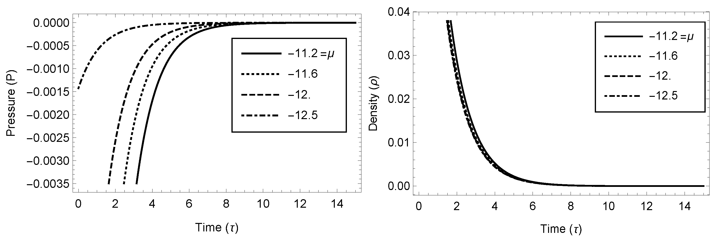
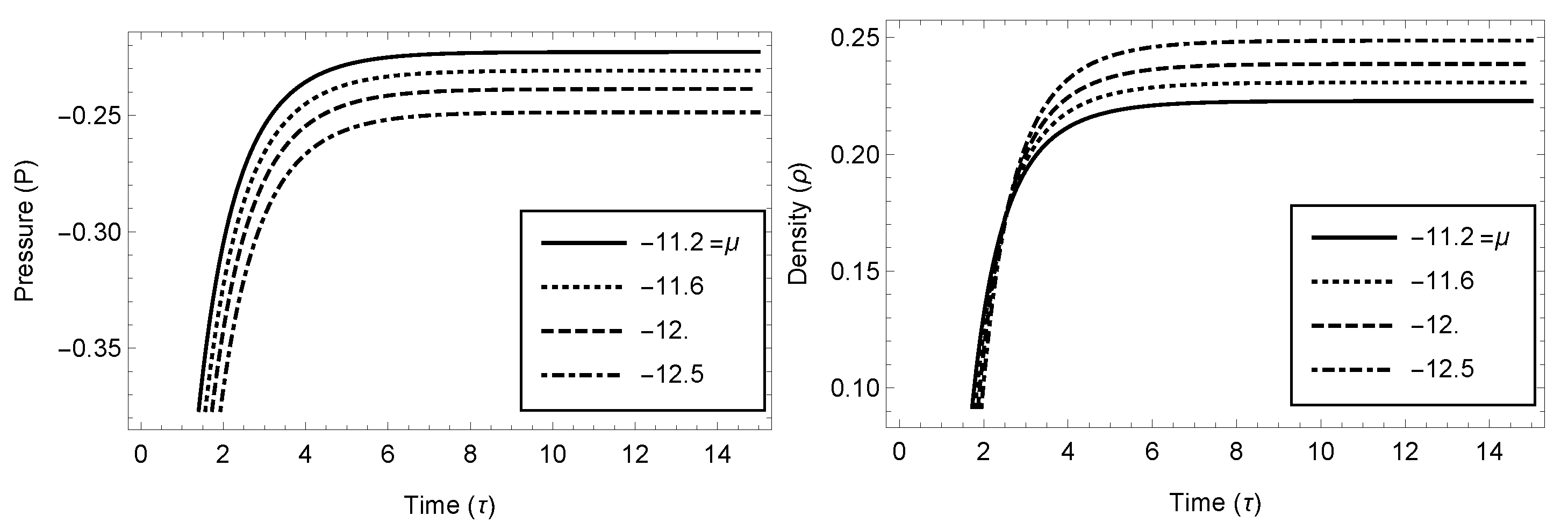
The cosmic distribution has a finite fluid pressure and matter density at $\tau =0$. The physical quantities decrease as $\tau$ increases and tend to zero when $\tau \to \infty$. Thus, our presented model leads to a vacuum cosmological solution at infinite time.

(3)

As $\frac{{\sigma }^2}{{\theta }^2}\ne 0$, so the model is anisotropic throughout the evolution. Again, $\tau \to \infty$ exhibits the expanding universe. However, $q=3$ dictates that the universe is decelerating.

(4)

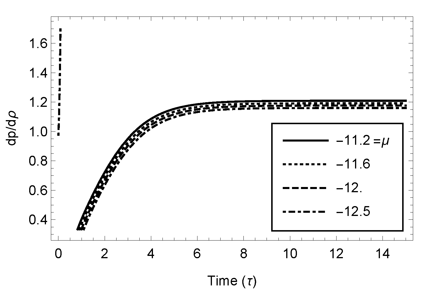
The stability of the model is obtained by considering the ratio $\frac{dp}{d\rho }$, which is positive for $\mu >-4\pi$, to yield a stable model.

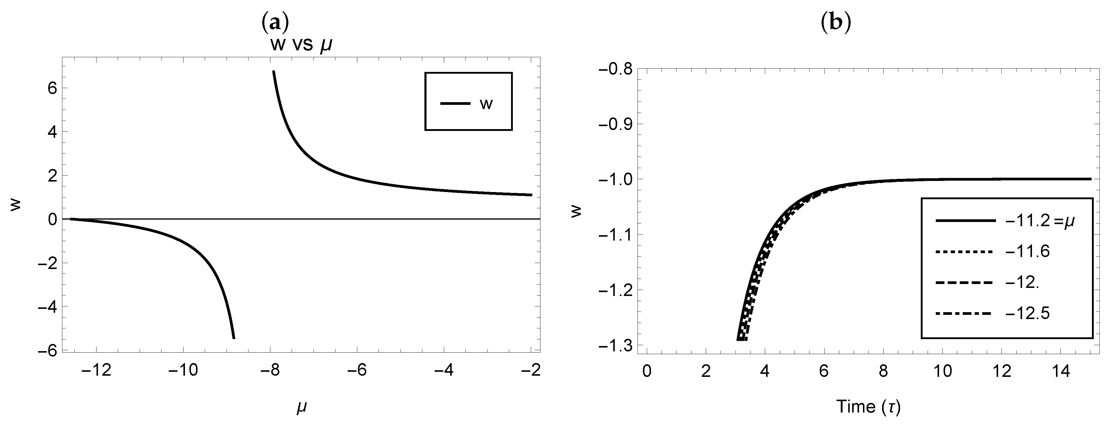
(5)

The EOS parameter is governed by the parameter $\mu$, and its value can be found as $\mu <-3.2\pi$. This is related to $w<-1$, which behaves like a phantom-energy-inspired cosmology. This type of phantom cosmology allows us to account for the dynamics and matter content of the universe, tracing back the evolution to the inflationary epoch [74]. In this connection, we would also like to point out that while the dependence of $\mu$ is explicit across all cases, this is not overall true, as this situation is solely visible in the results from Case 3.1. One can note that Case 3.3 shows a clear time dependence (and therefore, very dependent on the magnitude of $c_2$).

(6)

The anisotropic/isotropic behavior of the models for different choices of the parameters are given in Table 1 in connection with Case 3.2.

Thus, an obvious issue is here: how to incorporate an accelerating phase of the universe, which is the present cosmological scenario, along with the decelerating phase in our phantom-type dark energy model. However, following Capozziello et al. [75], one can make an endeavor to obtain a transition from the deceleration to the acceleration phase of the universe. Therefore, this issue can be addressed in a future project.

References

- Minkowski, H. Die Grundgleichungen für die Elektromagnetischen Vorgänge in bewegten Körpern. Wissenschaften zu Göttingen, Mathematisch-Physikalische 1908, 1908, 53–111. [Google Scholar]
- Minkowski, H. Jahresbericht der Deutschen Mathematiker-Vereinigung. Raum und Zeit 1909, 18, 75–88. [Google Scholar]
- Landau, L.D.; Lifshitz, E.M. The Classical Theory of Fields. Course of Theoretical Physics, 4th ed.; Butterworth-Heinemann: Oxford, UK, 2002; Volume 2. [Google Scholar]
- Kaluza, T. Zum Unitätsproblem in der Physik. Sitz. Preuss. Akad Wiss. 1921, 33, 966–972. [Google Scholar]
- Klein, O. Quantentheorie und fünfdimensionale Relativitätstheorie. Z. Phys. 1926, 37, 895–906. [Google Scholar] [CrossRef]
- Chodos, A.; Detweiler, S. Where has the fifth dimension gone? Phys. Rev. D 1980, 21, 2167–2170. [Google Scholar] [CrossRef]
- Alvarez, E.; Gavela, M.B. Entropy from Extra Dimensions. Phys. Rev. Lett. 1983, 51, 931–934. [Google Scholar] [CrossRef]
- Marciano, W.J. Time Variation of the Fundamental “Constants" and Kaluza–Klein Theories. Phys. Rev. Lett. 1984, 52, 489–491. [Google Scholar] [CrossRef]
- Gegenberg, J.D.; Das, A. Five-dimensional cosmological models with massless scalar fields. Phys. Lett. 1985, 112A, 427–430. [Google Scholar] [CrossRef]
- Lorenz-Petzold, D. Higher-dimensional extensions of Bianchi type-I cosmologies. Phys. Rev. 1985, 31, 929–931. [Google Scholar] [CrossRef]
- Wesson, P.S. Astrophysical data and cosmological solutions of a Kaluza–Klein theory of gravity. Astron. Astrophys. 1986, 166, 1–3. [Google Scholar]
- Grøn, Ø. Inflationary cosmology according to Wesson’s gravitational theory. Astron. Astrophys. 1988, 193, 1–4. [Google Scholar]
- Wesson, P. 5-Dimensional Physics: Classical and Quantum Consequences of Kaluza Klein Cosmology; World Scientific Publishing Company: Singapore, 2006. [Google Scholar]
- Abbott, R.B.; Barr, S.M.; Ellis, S.D. Kaluza-Klein cosmologies and inflation. Phys. Rev. D 1984, 30, 720–727. [Google Scholar] [CrossRef]
- Sahdev, D. Towards a realistic Kaluza-Klein cosmology. Phys. Lett. 1984, 137B, 155–159. [Google Scholar] [CrossRef]
- Chatterjee, S.; Bhui, B. Homogeneous cosmological model in higher dimension. Mon. Not. R. Astron. Soc. 1990, 247, 57–61. [Google Scholar]
- Bergamini, R.; Orzalesi, C. Towards a cosmology for multidimensional unified theories. Phys. Lett. B 1984, 135, 38–42. [Google Scholar] [CrossRef]
- Ishihara, H. Kaluza-Klein Inflation. Prog. Theor. Phys. 1984, 72, 376–378. [Google Scholar] [CrossRef][Green Version]
- Banerjee, A.; Bhui, B.; Chatterjee, S. Bianchi type I cosmological models in higher dimensions. Astrophys. J. 1990, 358, 23–27. [Google Scholar] [CrossRef]
- Chatterjee, S.; Bhui, B.; Basu, M.B.; Banerjee, A. Inhomogeneous model with a cosmological constant. Phys. Rev. D 1994, 50, 2924–2927. [Google Scholar] [CrossRef]
- Banerjee, A.; Panigrahi, D.; Chatterjee, S. A class of inhomogeneous cosmological models in Kaluza–Klein spacetime. Class. Quantum Gravit. 1994, 11, 1405–1414. [Google Scholar] [CrossRef]
- Banerjee, A.; Das, A.; Panigrahi, D. Singularity-free cylindrically symmetric solutions in Kaluza-Klein space-time. Phys. Rev. D 1995, 51, 6816–6820. [Google Scholar] [CrossRef]
- Ledesma, D.S.; Bellini, M. Single field inflationary models with non-compact Kaluza–Klein theory. Phys. Lett. B 2004, 581, 1–8. [Google Scholar] [CrossRef]
- Aguilar, J.E.M.; Bellini, M. Noncompact Kaluza–Klein theory and inflationary cosmology: A complete formalism. Phys. Lett. B 2004, 596, 116–122. [Google Scholar] [CrossRef][Green Version]
- Bellini, M. Inflationary cosmology from STM theory of gravity. Nucl. Phys. B 2003, 660, 389–400. [Google Scholar] [CrossRef]
- Liko, T.; Wesson, P.S. An exact solution of the five-dimensional Einstein equations with four-dimensional de Sitter-like expansion. J. Math. Phys. 2005, 46, 062504. [Google Scholar] [CrossRef]
- Mukhopadhyay, U.; Ghosh, P.P.; Ray, S. Higher dimensional dark energy investigation with variable Λ and G. Int. J. Theor. Phys. 2010, 49, 1622–1627. [Google Scholar] [CrossRef][Green Version]
- Sharif, M.; Khanum, F. Kaluza-Klein cosmology with varying G and Λ. Astrophys. Space Sci. 2011, 334, 209–214. [Google Scholar] [CrossRef][Green Version]
- Pahwa, I. Higher dimensional cosmological models: An alternative explanation for late time cosmic acceleration. J. Phys. Conf. Ser. 2014, 484, 012045. [Google Scholar] [CrossRef]
- Perlmutter, S.; Aldering, G.; Della Valle, M.; Deustua, S.; Ellis, R.S.; Fabbro, S.; Fruchter, A.; Goldhaber, G.; Groom, D.E.; Hook, I.M.; et al. Discovery of a supernova explosion at half the age of the Universe. Nature 1998, 391, 51–54. [Google Scholar] [CrossRef]
- Perlmutter, S.; Aldering, G.; Goldhaber, G.; Knop, R.A.; Nugent, P.; Castro, P.G.; Deustua, S.; Fabbro, S.; Goobar, A.; Groom, D.E.; et al. Measurements of Ω and Λ from 42 high-redshift supernovae. Astrophys. J. 1999, 517, 565–586. [Google Scholar] [CrossRef]
- Knop, R.A.; Aldering, G.; Amanullah, R.; Astier, P.; Blanc, G.; Burns, M.S.; Conley, A.; Deustua, S.E.; Doi, M.; Ellis, R.; et al. New constraints on ΩM, ΩΛ, and w from an independent set of 11 high-redshift supernovae observed with the Hubble Space Telescope. Astrophys. J. 2003, 598, 102–137. [Google Scholar] [CrossRef]
- Riess, A.G.; Filippenko, A.V.; Challis, P.; Clocchiatti, A.; Diercks, A.; Garnavich, P.M.; Gilliland, R.L.; Hogan, C.J.; Jha, S.; Kirshner, R.P.; et al. Observational evidence from supernovae for an accelerating Universe and a cosmological constant. Astron. J. 1998, 116, 1009–1038. [Google Scholar] [CrossRef]
- Riess, A.G.; Strolger, L.-G.; Tonry, J.; Casertano, S.; Ferguson, H.C.; Mobasher, B.; Challis, P.; Filippenko, A.V.; Jha, S.; Li, W.; et al. Type Ia supernova discoveries at z > 1 from the Hubble Space Telescope: Evidence for past deceleration and constraints on dark energy evolution. Astron. J. 2004, 607, 665–687. [Google Scholar] [CrossRef]
- Tonry, J.L.; Schmidt, B.P.; Barris, B.; Candia, P.; Challis, P.; Clocchiatti, A.; Coil, A.L.; Filippenko, A.V.; Garnavich, P.; Hogan, C.; et al. Cosmological results from high-z supernovae. Astron. J. 2003, 594, 1–24. [Google Scholar] [CrossRef]
- Valentino, E.D.; Mena, O.; Pan, S.; Visinelli, L.; Yang, W.; Melchiorri, A.; Mota, D.F.; Riess, A.G.; Silk, J. In the realm of the Hubble tension—a review of solutions. Class. Quantum Grav. 2021, 38, 153001. [Google Scholar] [CrossRef]
- Valentino, E.D. Challenges of the standard cosmological model. Universe 2022, 8, 399. [Google Scholar] [CrossRef]
- Harko, T.; Lobo, F.S.N.; Nojiri, S.; Odintsov, S.D. f(R, T) gravity. Phys. Rev. D 2011, 84, 024020. [Google Scholar] [CrossRef]
- Capozziello, S.; Laurentis, M.D. Extended theories of gravity. Phys. Rep. 2011, 509, 167–321. [Google Scholar] [CrossRef]
- Adhav, K.S. LRS Bianchi type-I cosmological model in f(R, T) theory of gravity. Astrophys. Space Sci. 2012, 339, 365–369. [Google Scholar] [CrossRef]
- Alvarenga, F.G.; Houndjo, M.J.S.; Monwanou, A.V.; Orou, J.B.C. Testing some f(R, T) gravity models from energy conditions. J. Mod. Phys. 2013, 4, 130–139. [Google Scholar] [CrossRef]
- Mahanta, K.L. Bulk viscous cosmological models in f(R, T) theory of gravity. Astrophys. Space Sci. 2014, 353, 683–689. [Google Scholar] [CrossRef]
- Mishra, B.; Sahoo, P.K. Bianchi type VIh perfect fluid cosmological model in f(R, T) theory. Astrophys Space Sci. 2014, 352, 331–336. [Google Scholar] [CrossRef]
- Cai, Y.-F.; Capozziello, S.; Laurentis, M.D.; Saridakis, E.N. f(T) teleparallel gravity and cosmology. Rept. Prog. Phys. 2016, 79, 106901. [Google Scholar] [CrossRef] [PubMed]
- Das, A.; Rahaman, F.; Guha, B.K.; Ray, S. Compact stars in f(R, T) gravity. Eur. Phys. J. C 2016, 76, 654. [Google Scholar] [CrossRef]
- Das, A.; Ghosh, S.; Guha, B.K.; Das, S.; Rahaman, F.; Ray, S. Gravastars in f(R, T) gravity. Phys. Rev. D 2017, 95, 124011. [Google Scholar] [CrossRef]
- Moraes, P.H.R.S.; Sahoo, P.K. Modeling wormholes in f(R, T) gravity. Phy. Rev. D 2018, 97, 024007. [Google Scholar] [CrossRef]
- Mishra, B.; Tripathy, S.K.; Tarai, S. Cosmological models with a hybrid scale factor in an extended gravity theory. Mod. Phys. Lett. A 2018, 33, 1850052. [Google Scholar] [CrossRef]
- Deb, D.; Guha, B.K.; Rahaman, F.; Ray, S. Anisotropic strange stars under simplest minimal matter-geometry coupling in the f(R, T) gravity. Phys. Rev. D 2018, 97, 084026. [Google Scholar] [CrossRef]
- Deb, D.; Rahaman, F.; Ray, S.; Guha, B.K. Strange stars in f(R, T) gravity. J. Cosmol. Astropart. Phys. 2018, 03, 044. [Google Scholar] [CrossRef]
- Biswas, S.; Ghosh, S.; Guha, B.K.; Rahaman, F.; Ray, S. Strange stars in Krori–Barua spacetime under f(R, T) gravity. Ann. Phys. 2019, 401, 1–20. [Google Scholar] [CrossRef]
- Deb, D.; Ketov, S.V.; Khlopov, M.; Ray, S. Study on charged strange stars in f(R, T) gravity. J. Cosmol. Astropart. Phys. 2019, 10, 070. [Google Scholar] [CrossRef]
- Deb, D.; Ketov, S.V.; Maurya, S.K.; Khlopov, M.; Moraes, P.H.R.S.; Ray, S. Exploring physical features of anisotropic strange stars beyond standard maximum mass limit in f(R, T) gravity. Mon. Not. R. Astron. Soc. 2019, 485, 5652–5665. [Google Scholar] [CrossRef]
- Fisher, S.B.; Carlson, E.D. Reexamining f(R, T) gravity. Phys. Rev. D 2019, 100, 064059. [Google Scholar] [CrossRef]
- Biswas, S.; Shee, D.; Ray, S.; Guha, B.K. Anisotropic strange star with Tolman–Kuchowicz metric under f(R, T) gravity. Eur. Phys. J. C 2020, 80, 175. [Google Scholar] [CrossRef]
- Ray, S.; Sengupta, R.; Nimesh, H. Gravastar: An alternative to black hole. Int. J. Mod. Phys. D 2020, 29, 2030004. [Google Scholar] [CrossRef]
- Hulke, N.; Singh, G.P.; Bishi, B.K.; Singh, A. Variable Chaplygin gas cosmologies in f(R, T) gravity with particle creation. New Astron. 2020, 77, 101357. [Google Scholar] [CrossRef]
- Mishra, B.; Esmeili, F.M.; Ray, S. Cosmological models with variable anisotropic parameter in f(R, T) gravity. Ind. J. Phys. 2021, 95, 2245–2254. [Google Scholar] [CrossRef]
- Varshney, G.; Sharma, U.K.; Pradhan, A.; Kumar, N. Reconstruction of Tachyon, Dirac-Born-Infeld-essence and Phantom model for Tsallis holographic dark energy in f(R, T) gravity. Chin. J. Phys. 2021, 73, 56–73. [Google Scholar] [CrossRef]
- Pradhan, A.; Garg, P.; Dixit, A. FRW cosmological models with cosmological constant in f(R, T) theory of gravity. Can. J. Phys. 2021, 99, 741–753. [Google Scholar] [CrossRef]
- Bhardwaj, V.K.; Pradhan, A. Evaluation of cosmological models in gravity in different dark energy scenario. New Astron. 2022, 91, 101675. [Google Scholar] [CrossRef]
- Tiwari, R.K.; Beesham, A.; Mishra, S.; Dubey, V. Bianchi type I cosmological model in f(R, T) gravity. Phys. Sci. Forum 2021, 2, 38. [Google Scholar] [CrossRef]
- Tiwari, R.K.; Beesham, A.; Mishra, S.; Dubey, V. Anisotropic cosmological model in a modified theory of gravitation. Universe 2021, 7, 226. [Google Scholar] [CrossRef]
- Bertolami, O.; Lobo, F.S.N.; Paramos, J. Nonminimal coupling of perfect fluids to curvature. Phys. Rev. D 2008, 78, 064036. [Google Scholar] [CrossRef]
- Schutz, B.F. Perfect fluids in general relativity: Velocity potentials and a variational principle. Phys. Rev. D 1970, 2, 2762. [Google Scholar] [CrossRef]
- Brown, J.D. Action functionals for relativistic perfect fluids. Class. Quantum Gravit. 1993, 10, 1579. [Google Scholar] [CrossRef]
- Baffou, E.H.; Houndjo, M.J.S.; Rodrigues, M.E.; Kpadonou, A.V.; Tossa, J. Cosmological evolution in f(R, T) theory with collisional matter. Phys. Rev. D 2015, 92, 084043. [Google Scholar] [CrossRef]
- Mohanty, G.; Sahoo, R.R. Mesonic stiff fluid distribution in five dimensional Bianchi type space time. Astrophys. Space Sci. 2008, 314, 1–6. [Google Scholar] [CrossRef]
- Collins, C.B.; Glass, E.N.; Wilkinson, D.A. Exact spatially homogeneous cosmologies. Gen. Relativ. Gravit. 1980, 12, 805–823. [Google Scholar] [CrossRef]
- Moraes, P.H.R.S. Cosmology from induced matter model applied to 5D f(R, T) theory. Astrophys. Space Sci. 2014, 352, 273–279. [Google Scholar] [CrossRef]
- Borkar, M.S.; Ameen, A. Evaluation of Bianchi type VI0 magnetized anisotropic dark energy models with constant deceleration parameter in bimetric theory of gravitation. Int. J. Mod. Phys. D 2015, 24, 1550019. [Google Scholar] [CrossRef]
- Caldwell, R.R. A phantom menace? Cosmological consequences of a dark energy component with super-negative equation of state. Phys. Lett. B 2002, 545, 23–29. [Google Scholar] [CrossRef]
- Caldwell, R.R.; Kamionkowski, M.; Weinberg, N.N. Phantom energy: Dark energy with w < −1 causes a cosmic doomsday. Phys. Rev. Lett. 2003, 91, 071301. [Google Scholar] [CrossRef] [PubMed]
- Capozziello, S.; Nojiri, S.; Odintsov, S.D. Unified phantom cosmology: Inflation, dark energy and dark matter under the same standard. Phys. Lett. B 2006, 632, 597–604. [Google Scholar] [CrossRef]
- Astashenok, A.V.; Nojiri, S.; Odintsov, S.D.; Yurov, A.V. Phantom cosmology without Big Rip singularity. Phys. Lett. B 2012, 709, 396–403. [Google Scholar] [CrossRef]