Modeling of Solar Wind Disturbances Associated with Coronal Mass Ejections and Verification of the Forecast Results

Abstract

Solar wind (SW) disturbances associated with coronal mass ejections (CMEs) cause significant geomagnetic storms, which may lead to the malfunction or damage of sensitive on-ground and space-based critical infrastructure. CMEs are formed in the solar corona, and then propagate to the Earth through the heliosphere as Interplanetary CME (ICME) structures. We describe the main principles in development with the online, semi-empirical system known as the Space Monitoring Data Center (SMDC) of the Moscow State University, which forecasts arrival of ICMEs to Earth. The initial parameters of CMEs (speeds, startup times, location of the source) are determined using data from publicly available catalogs based on solar images from space telescopes and coronagraphs. After selecting the events directed to Earth, the expected arrival time and speed of ICMEs at the L1 point are defined using the Drag-Based model (DBM), which describes propagation of CMEs through the heliosphere under interaction with the modeled quasi-stationary SW. We present the test results of the ICME forecast in the falling phase of Cycle 24 obtained with the basic version of SMDC in comparison with results of other models, its optimization and estimations of the confidence intervals, and probabilities of a successful forecast.

1. Introduction

Since the discovery of solar wind (SW) in 1960s [1,2], it was discovered that transient anomalies of the SW stream associated with solar eruptions may cause disturbances in the near-Earth space due to the release of considerable energy from SW to the Earth’s magnetosphere. These disturbances can be harmful to modern on-ground and space-based technical systems due to their high sensitivity, complexity, and global interrelationship. The main task of the space weather forecasting system is to warn about the appearance of significant SW disturbances in near-Earth space and beyond, in order to prevent the malfunction or even destruction of sensitive technological systems on Earth and in space. Online tools based on the data of regular solar observations can provide the information needed to protect these systems from probable geomagnetic effects in advance of two to five days.

Regular observations of the SW parameters by dedicated spacecraft reveal the SW disturbances as enhancements of the magnetic field strength, flow speed, density, and composition of the SW plasma. Commonly, (see, e.g., [3,4] and the references therein), in near-Earth space the SW disturbances are considered in relation to three basic types of SW: (1) High-speed streams (HSSs) associated with coronal holes (CHs); (2) Slow, inter-stream SW (SSWs); and (3) Transient flows associated with coronal mass ejections (CMEs) of two types—magnetic clouds and ejecta, revealed in the heliosphere as interplanetary coronal mass ejections (ICMEs). In addition, there are other important, shorter-time SW features as shocks, magnetic stream interface regions (SIRs), co-rotating interaction regions (CIRs), sheaths (plasma density enhancements), and heliospheric current sheets. The mentioned features have specific signatures [4,5,6], although, due to the interaction of different streams in the heliosphere, some signatures may be only partly expressed or fully absent [7,8].

When the SW irregularities approach Earth, they may disturb the magnetosphere, sometimes causing geomagnetic storms. The strongest geomagnetic disturbances are associated with one, or a sequence of, CMEs. According to the data presented in the catalog of the Space Research Institute, Moscow, described in [4], in the period 1976–2000 (solar cycles 21–23) the largest geo-effectiveness was observed for CMEs (magnetic clouds with sheaths)—61%, for CIR and ejecta with sheaths −20–21%, for sheaths alone—15%, and ejecta without sheath—8%. Some other results from the statistical analysis of the CME geo-effectiveness in different phases of the solar activity can be found in [9,10,11,12,13].

Since the efforts of modeling the CME magnetic structure are not currently enough successful [14,15,16,17], a reliable forecast of the SW geo-effectiveness is currently possible only from the in-situ measurements of SW parameters at near-Earth orbit. The task of the online CME forecasting system is to provide a warning of the CME arrival time and speed at the L1 point within the reasonable waiting interval of 12–24 h. When the forecasted CME arrives to L1 and the in-situ SW measurements confirm its geo-effectiveness, the alarm of the geomagnetic storm is issued with the clarified time of its appearance and estimated significance.

Quasi-stationary SW streams (QSW) consisting of HSS and SSW are the most important components of the interplanetary environment where CMEs propagate. SSWs with velocities varying from about 250 to 350–400 km s⁻¹ and HSSs with velocities from about 400 to 900 km s⁻¹ constitute the background SW, which governs propagation of CMEs in the heliosphere by accelerating or decelerating them. Therefore, modeling of QSW is an important part of the ICME prediction.

At present, there are several models for predicting the parameters of QSW. Quite often, empirical relationships are implemented that connect solar coronal or photospheric parameters determined from magnetic field or radiation measurements to the speed of QSWs at several solar radii (R_Sun), and then recalculate to 1 AU. The most well-known is a semi-empirical Wang-Sheeley-Arge (WSA) model [18,19]. The WSA model is based on the photospheric magnetograms and calculations of the magnetic field on the source surface in the potential field source surface (PFSS) approximation.

A number of other empirical models predict QSW speed based on the analysis of the parameters of CHs; the regions of open configuration of the photospheric magnetic field lines. Extensive CHs extended to low solar latitudes are the coronal sources of QSWs observed in near-Earth orbit for several days, or even weeks [20]. Such models often use images of the Sun in the extreme ultraviolet region of the spectrum (e.g., [21,22,23,24]). For long-term modeling QSW, some of the models use the measured SW parameters in near-Earth orbit obtained during previous solar rotations [25].

Simulation of the CME/ICME propagation by any model embraces localization of the primary CME source at the Sun; selection of the events directed to Earth and modeling a passage of CME in the heliosphere taking into account its probable interaction with QSW and other CMEs. Origination of CMEs in the solar corona is associated with spontaneous eruption of the coronal plasma, which can be revealed from regular solar observations by specific signatures such as coronal dimmings, expanding loop structures in the low corona seen by extreme ultraviolet (EUV) telescopes, and expanding regions of density enhancements seen by coronagraphs.

Coronal dimmings, localized regions of reduced emission in extreme ultraviolet and soft X-rays, are interpreted as density depletions due to mass loss during the CME expansion in the lower corona (e.g., [6,7,8]). Dimmings provide important information on the initiation and early evolution of CMEs before they appear in coronagraphs. The formation and properties of dimmings were studied in many publications (see, e.g., [26,27,28,29,30]. The relationship between the parameters of the dimming regions and the associated CMEs have been analyzed in several studies (e.g., [31,32,33]). All of the necessary information about dimmings starting from May, 2010 has been gathered by Solar Demon software [34], which automatically detects and characterizes dimmings in a semi-automatic way by analysis of the images obtained by the Atmospheric Imaging Assembly EUV telescope at the Solar Dynamic Observatory (SDO/AIA) in the 21.1 nm band. Detections are performed both in near real-time on quick-look data, as well as on synoptic science data to generate event catalogs.

The developing CMEs appear in the coronagraph’s field of view (above ~2 R_Sun) as expanding plasma structures accelerate or decelerate in the upper corona [35,36,37]. Analysis of coronagraphic images [38] enables the determination of the speeds and masses of CMEs. However, it only gives expansion speed in projection to the plane-of-sky. The radial component of the CME speed can be restored from the expansion speed in the frames of some geometrical models, like the cone model or the “Ice-cream” model [39,40]. However, most of the geo-effective CMEs moving towards the Earth are wide, and according to the cone-type model, Earth-directed speed does not differ significantly from the expansion speed [39].

The ICME kinematics in the heliosphere depend on the CME speed, mass, and size as well as on the background (ambient) SW density and velocity. To describe the propagation of CMEs/ICMEs in interplanetary space, the Drag-Based Model (DBM, [41,42,43,44,45,46,47,48,49]) is widely used due to its simplicity and low computational cost. This model assumes that from a certain distance from the Sun (typically, at R ≥ 20 R_Sun), where the Lorentz and gravity forces become negligible, the CME dynamics are governed by magnetohydrodynamic drag produced by the interaction of the CME plasma with the interplanetary ambient SW. The application of DBM for modeling CME propagation in the heliosphere is considered in recent publications [49,50,51,52].

The aim of the current research is to consider the modeling approaches and their realization in the developing online forecasting Space Monitoring Data Center (SMDC) system for the forecast of the SW disturbances associated with the ICMEs near the Earth, based on the data of regular solar observations accumulated in the available databases. We describe the basic approaches used in the SMDC realization and the results of its application on the events in 2015–2017. In Chapter 2 (Data and Methods) we consider the data sources, principles of the forecasting procedure, and a choice of the input data and the model parameters. In Chapter 3 (Results) we describe the results of validation of the basic SMDC system, their comparison with the results of other models, optimization of SMDC using the ensemble approach, and estimations of the confidence intervals of successive forecasts. In Chapter 4 (Discussion) we analyze the probable causes of missing and false predictions, and consider possibilities to adjust the SMDC according with current solar conditions. The final remarks are given in Conclusion.

2. Data and Methods

2.1. Main Principles of SMDC and Sources of the Input Data

Until now, efforts to create a full-scale digital or physical operational model to predict geomagnetic storms with sufficient accuracy based on the currently available solar observations were not successful enough. The main cause is that the evolution of the SW magnetic structure in the upper corona and in the inner heliosphere is poorly understood due to the lack of direct observations (the investigations of the Parker Solar Probe and Solar Orbiter missions inspire good hope). Additionally, the propagation of SW streams in the corona and heliosphere takes place in sufficiently different conditions, so it cannot be described by a single physical model. Under these circumstances, the best method is to divide the whole task into several successive parts: the coronal part, the heliospheric part, and the geomagnetic part, which have different space and temporal scales. The coronal part extends in distance from 0.1 to ~20 R_Sun from the Sun with a duration of several hours to half of a day, the heliospheric part—extends in distance from 20 to 215 R_Sun with a duration of 1 to 5 days, and the geomagnetic part—from 10 to 1 R_Earth from the Earth with duration from ~2 h to 1 day [53].

In the coronal part, optical observations of the coronal structures by space telescopes and coronagraphs provide data about the appearance and formation of SW streams, which further propagate in the heliosphere. Near the Earth, typically in the L1 point, measurements of the temporal profiles of the SW plasma and magnetic field parameters allow the forecasting of the following geomagnetic effects with high reliability. Thus, the most critical element for the determination of the onset time of geomagnetic effects associated with CMEs is the heliospheric part, where propagation of the SW disturbances may be modeled using the initial data obtained from the coronal observations, taking into account their probable interaction with the streams from other solar sources.

Thus, the online forecasting system that is under development should contain two parts. The first, coronal part is based on regular images from SDO/AIA [54], available from the Joint Science Operations Center (JSOC) database (http://jsoc.stanford.edu (accessed on 20 September 2022)), and from The Large Angle Spectrometric COronagraph (LASCO) onboard the Solar and Heliospheric Observatory (SOHO) [55]). The CME data obtained from the LASCO images are presented in the automatically processed Computer Aided CME Tracking (CACTus) LASCO CME catalog (https://www.sidc.be/cactus (accessed on 20 September 2022)) and in the Coordinated Data Analysis Workshop (CDAW) catalog (https://cdaw.gsfc.nasa.gov/CME_list (accessed on 20 September 2022)). A detailed comparison of the CACTus and CDAW data for the solar cycles 23 and 24 is given in [56].

Information concerning the onset time and location of the CME-associated dimmings are taken from the Solar Demon catalog (http://solardemon.oma.be, [34] (accessed on 20 September 2022)). The Solar Demon website contains a summary of the dimmings, providing the start, peak, and end time of the dimming, the latitude and longitude of its barycenter, the intensity change over time, details about the nearest active region, and the area of the dimming for each event. The parameters of dimmings taken from Solar Demon are used for preliminary filtering of the events in order to distinguish the Earth-directed CMEs. The details concerning the event selection are considered below.

The time and speed of the appearance of the selected CME-associated flows in the coronagraphic images are used in the second part of the prediction procedure—modeling of the CME propagation in the heliosphere. For this purpose, we used the basic version of DBM [41,42,43,44] founded on the equation for the drag force acceleration:

$$\frac{dV}{dT}=-\gamma (v-w) |v-w|,$$

(1)

where v is the CME velocity and w represents the ambient SW speed (in km s⁻¹), γ (in km⁻¹) is the drag parameter (see e.g., [42,45,46]). The online version of the DBM is available at the site https://oh.geof.unizg.hr/DBM/dbm.php (accessed on 24 October 2022). The initial parameters for simulation include: the time and speed of the CME-related flows at the distance R = 20 R_Sun (T₂₀, V₂₀), the speed w of the background SW, and the drag parameter γ. The typical error of the DBM method in its basic form can be estimated as ±10 h (in time) and ±50 km s⁻¹ (in speed) [47,48]. These errors depend on uncertainties in the measured initial CME speed, in the speed of ambient SW along the path of CME in the heliosphere, and unknown drag coefficient. Typically, the values of γ are taken in the range from 1 × 10⁻⁸ km⁻¹ (in the cases of bright massive CMEs in the fast solar-wind environment with low density) up to 2 × 10⁻⁷ km⁻¹ (in the cases of low-density CMEs in the SSW [44,46]).

To validate the prediction results, we compared the predicted arrival time and speed of ICMEs with the measured values using two main databases: the Richardson and Cane ICME list (https://izw1.caltech.edu/ACE/ASC/DATA/level3/icmetable2.html (accessed on 20 September 2022)). [57], hereafter the R&C list) based on the data of the Advanced Composition Explorer (ACE, [58]), and the catalog of solar events of the Space Research Institute, Moscow, Russia (SRI, http://www.iki.rssi.ru/pub/omni (accessed on 20 September 2022), [59]), based on the OMNI data (https://omniweb.gsfc.nasa.gov (accessed on 20 September 2022)). We compared a quality of the SMDC forecasts with the results of other semi-empirical and numerical prediction models presented at the CME Scoreboard site of NASA Coordinated Modeling Center (CCMC, https://ccmc.gsfc.nasa.gov/scoreboards/cme (accessed on 20 September 2022)).

2.2. Identification of the CME Sources and Selection of Events for Analysis

We determined the initial parameters of a CME for the SMDC system using the CACTus data [60]. However, the total number of events in the CACTus database (i.e., in 2017 year it contains 369 events) is much greater than the number of ICMEs in the R&C list (in 2017—9 events). CACTus contains many narrow events with an angular width (da) less than 20 degrees (57% of all events for 2017). Such narrow CMEs are more likely associated with the non-geo-effective ICME-like structures or enhancements of the slow SW in contrast to the wider geo-effective CMEs [61]. Thus, it is necessary to apply the preliminary selection of the CMEs directed to the Earth with considerable geo-effectiveness propagating in the ecliptic plane and having significant angular width.

This selection can be applied after the determination of the CME sources as an important part of the CME propagation modeling. The coronagraphic data do not contain the necessary information about the CME direction, because the events propagating toward the Earth are indiscernible from those moving in the opposite direction. Such selection can be provided by using multi-coronagraph observations, but such data are available only for special periods (i.e., by using the instruments onboard the Solar TErrestrial RElations Observatory, STEREO-A and B spacecraft for 2008–2013). To address this issue, one could use information about dimmings that are observed in the solar corona as a result of eruption as being indicative of the CME source on the Solar disk. For this purpose, we used a special CME selection algorithm, which includes the application of four filters based on both the CME parameters and the characteristics of the CME-dimming correspondence.

• Step 1: CME merging

The CACTus software, in some cases, detects a series of separated CME-like events. To avoid ambiguity, we merge all events starting simultaneously (within ± 50 min) with overlapping angular parameters. Then, we compare all merging events by their angular width (da) and position angle (pa). The position angle pa is defined as the angle between the north (0 degrees) and the center of the CME angular profile, measured counterclockwise in the picture plane. If one of the CMEs is sufficiently wider than the others (e.g., halo or partial halo), we select this one. In the other case, the temporal parameters of the merged CMEs are defined as follows: CME start time: t_start = MIN(t_start_i), CME end time: t_end = MAX(t_end_i), CME duration: dt = t_end–t_start, where t_start_i and t_end_i are the values of start and end times of the individual merged CMEs. The da value of the merged CMEs is determined by the uttermost points of the total angular profile, the pa-value—by its middle point.

• Step 2: Angular CME filter

After the CME merging, we remove narrow events depending on their position angle. We regard events as equatorial if their pa is in the range of (60, 120) or (240, 300) degrees, the other events we regard as polar. Finally, we select the equatorial CMEs with da ≥ 30° and the polar CMEs with da ≥ 60°.

• Step 3: CME-dimming correspondence

Dimmings are observed in the solar corona earlier than CMEs reach the coronagraph field of view, and this time delay depends on the CME velocity and geometry. According to statistical and case studies, this time delay constitutes from several minutes to a few hours depending on the CME and instrument parameters. Harrison et al. [8] analyzed the LASCO data for CMEs and the CDS instrument onboard SOHO for dimmings in 15–80 nm spectral range. They found the minimum time delay of 40 min and maximum of more than 3 h. In SMDC we assume that the dimmings should be observed in less than two hours earlier than the CME start time.

We also check the correspondence between the CME and dimming parameters. To make this examination, we compare the angle in the picture plane between the direction from the center of the solar disk to the dimming geometric center and direction to the north (counting counterclockwise) with the CME pa angle. If these angles match within 90 degrees, then the dimming—CME correspondence is established. If several suitable dimmings appeared, we select the event closest in time to the CME start time.

• Step 4: Filtering of the limb events

At this stage, we deselect all CMEs with sources that are located at the limb or on the opposite side of the Sun. For this purpose, we examine whether the average R_dist parameter of the dimming in Solar Demon (the distance of the dimming geometrical center from the center of the Solar disk divided on the solar radius) is less than 1. If R_dist ≥ 1, it means that the dimming is observed above the limb, its source is located on the limb or on the opposite side of the Sun evidently not directed to the Earth, so this event should be deselected. The results of application of the described filters are summarized in

Table 1. The number of events passed each step in the selection algorithm in the periods of 2015, 2016 and 2017.

Number of Events for Year	2015	2016	2017
CACTus (initial)	1730	922	580
Step 1	1505	854	555
Ratio 1, %	87	93	96
Step 2	341	188	134
Ratio 2, %	20	20	23
Step 3	144	42	30
Ratio 3, %	8	5	5
Step 4	82	22	14
Ratio 4, %	5	2	2

. The events passed the Step 4 filter we select for further processing, naming them as predicted events.

2.3. Modeling of the Background SW in the Heliosphere

The speed values of the background QSW, those of the initial parameters for DBM, were obtained using the SMDC empirical model of QSW (SMDC QSW) [23,62]. The model uses the parameters of coronal holes calculated from solar images from the SDO/AIA telescope at the wavelength of 19.3 nm providing a forecast of the hourly values of the QSW speed in the heliosphere up to 1 AU.

The areas of coronal holes are determined using a threshold algorithm for analyzing solar images. The QSW speed is modeled from the areas of coronal holes calculated from the region of the solar disk located near the central meridian (±20° in longitude and ±40° in latitude), according to the formula:

$$V\left(S,t\right)=V_{min}+A·S{\left(t_0\right)}^{\alpha }$$

(2)

where S(t₀) is the dimensionless relative area of CH situated within the zone distinguished by latitude and longitude at the time moment t₀ on the image in the 19.3 nm band; V_min is taken equal to 300 km s⁻¹ (the minimum speed calculated by the forecast algorithm in the absence of HSSs from CHs); A and α are the algorithm dimensionless parameters that are selected by minimizing modeling errors; t is the time of QSW arrival to the near-Earth orbit based on the speed forecast. In this model, the time of QSW propagation from the source surface to 1 AU is computed by ballistic model, where the QSW movement in the heliosphere is assumed to be uniform and radial. The QSW speed is calculated at several points of the heliosphere: 20 R_Sun, 65 R_Sun, 115 R_Sun, 165 R_Sun, and 215 R_Sun (1 AU) and can be used as an input parameter for DBM to simulate the ICME arrival time and speed. The forecast of QSW at 1 AU is posted in real time on the website of the Space Weather Analysis Center of the SINP MSU (https://swx.sinp.msu.ru/weather.php?lang=en (accessed on 20 September 2022)) [63]. The database of forecasts of the SW velocity starting from 2010 is also available from the SINP data analysis and visualization service (a screenshot is given in Figure 1) (https://swx.sinp.msu.ru/tools/davisat.php?gcm=1&lang=en (accessed on 25 August 2022)).

In the paper [62], we compare our QSW forecast results with the results of models used by other scientific groups for the 24th solar cycle. Data for comparison were taken from papers [21,64] for the periods 2011–2014 and 2011–2018, respectively. For the period 2011–2018, the correlation coefficient (CC) between the measured in-situ by ACE, and predicted by our model QSW velocities, is 0.44, and the root-mean square error (RMSE) is 96 km s⁻¹. These results of the QSW velocity forecast are comparable with the results of other empirical and semi-empirical models presented in the papers cited above. It should be mentioned that the forecast quality becomes worse for all models during the solar cycle maximum compared to the periods of rise, decline, and minimum. Thus, for the period 2011–2014, the CC value drops to 0.34, while the RMSE value increases to 98 km s⁻¹.

2.4. Modeling of CME Propagation in the Heliosphere by DBM

As it was mentioned in the Introduction, propagation of CMEs in the heliosphere can be modeled with the use of DBM, which is valid from the distance of 20 R_Sun from the Sun up to the Earth. The initial parameters of a CME for this modeling are the time and speed at 20 R_Sun, which can be obtained from the LASCO coronagraph images processed by CACTus. Because the CACTus database provides the CME parameters from 2 to 6 R_Sun, those are extrapolated to 20 R_Sun in assumption that the CME moves with constant speed between the distance of the first appearance (~5 R_Sun) to the final distance of 20 R_Sun.

In SMDC, we use the basic version of the Drag-based model, which offers the following solutions for the CME distance from the Sun r(t) and its speed v(t) [44]:

$$r\left(t\right)=\pm \frac{1}{\gamma }\ln \left(1\pm \gamma \left(v_0-w\right)t\right)+wt+r_0,$$

(3)

$$v\left(t\right)=w+\frac{v_0-w}{1\pm \gamma \left(v_0-w\right)t},$$

(4)

where w is the background SW speed (in km s⁻¹), $r_0$ = 20 R_Sun (≈1.39 × 10⁻⁷ km) and $v_0$ are the CME speed (in km s⁻¹) at the $r_0$, $\gamma$ is the drag parameter (in km⁻¹), t is the simulation time step equal to 1 h, “+” and “−” related to different modes of motion: deceleration ($v_0>w)$ and acceleration ($v_0<w)$ respectively.

According to the recommendations in [44], in the basic version of SMDC the drag parameter was set to the constant value specific for the different ranges of the CME speed: $\gamma$ = 1 × 10⁻⁸ km⁻¹ for $v_0>1000$ km s⁻¹; 2 × 10⁻⁸ km⁻¹ for $v_0\in \left[500,1000\right]$ km s⁻¹; 5 × 10⁻⁸ km⁻¹ for $v_0\le 500$ km s⁻¹. The speed w of the ambient SW is provided by the QSW model described above as a function of time in 4 space intervals 20–65 R_Sun, 65–115 R_Sun, 115–165 R_Sun and 165–215 R_Sun assuming to be constant inside their boundaries. When the CME, in its modeled motion, enters the next interval, the value of w in DBM changes to the corresponding value of the modeled QSW.

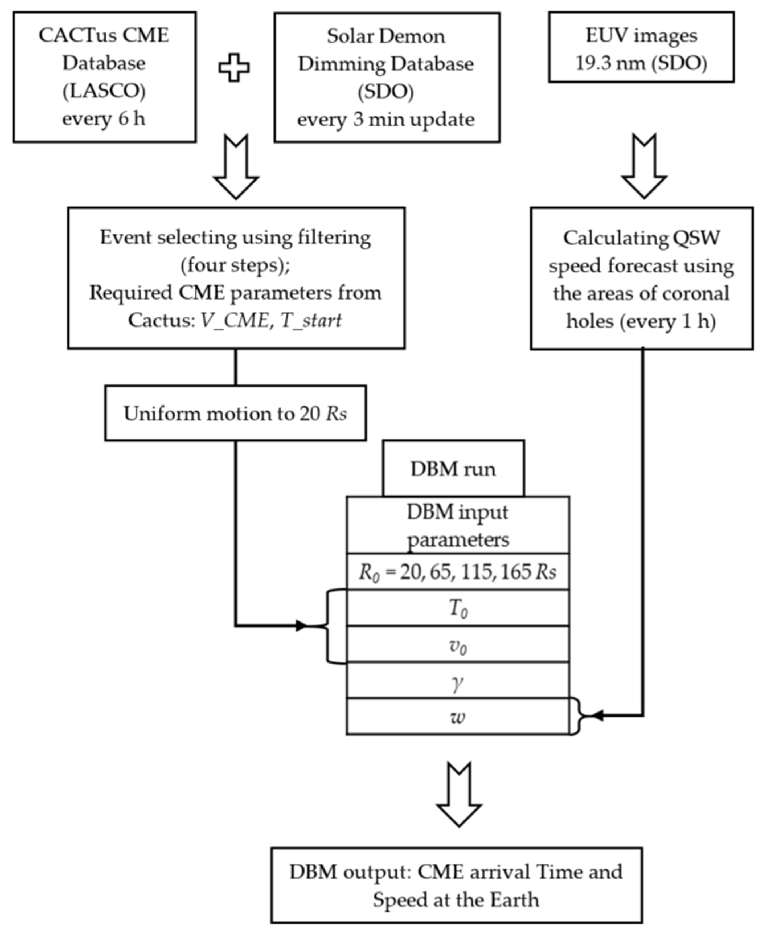
2.5. Scheme of Basic SMDC Forecasting System

The whole SMDC forecasting process is shown at the Figure 2. All necessary data are updated every day: the CACTus database has a quick look catalogue that is updated every 6 h, the Solar Demon Database also has the quick look page that is updated every 3 min. Thus, our selection method is available to run every 6 h to search for potentially significant CMEs. The startup CME time and speed are taken from the CACTus database after four-step filtering. Then, the initial parameters for DBM at 20 solar radii are determined in assumption of the uniform CME motion. The ambient SW speed w is calculated according to the QSW model taking the minimum value of 300 km s⁻¹ in the cases where no CHs are present at the solar disc.

All data from the external sites are automatically uploaded to the SMDC servers several times a day (presumably once every 6 h). After receiving fresh data, the forecast calculation program starts and the results appear at the web page of the CME forecast, which will then be created on the SINP MSU space weather website (https://swx.sinp.msu.ru/index.php?lang=en, accessed on 24 October 2022) in the section “Applications/Heliosphere”. This page contains information about the latest CMEs that meet the requirements of our selection method and the prediction of the speed and time of arrival of these CMEs into the Earth’s orbit. The whole calculation process runs on a personal computer quite fast; for example, it takes 2 min to process all the data for 2015.

3. Results

3.1. SMDC Test Results for 2015–2017 in Comparison with the ICME Catalogs and the CCMC Scoreboard Results

The period of 2015 was chosen due to the number of CMEs and geo-effective events. Since 2016, the number of CMEs has decreased, however, during the period 2016–2017 there were a large number of HSSs, so we learned how our system performs under different conditions. For adjusting and testing the algorithm of SMDC, we compared our results for 2015 with the observed data presented in the R&C list [57], which contains 29 events for that year. We also added 19 events indicated in the CCMC Scoreboard list [65] marked as reached the Earth. We compared the appearance time of the ICME coronal source indicated in the mentioned databases and considered that the ICME events should coincide within one hour. In the cases where the ICME source was absent in the R&C list, we consider the ICME events in these two bases as identical if their start times coincide within 24 h. After merging, we obtained 34 ICME events in total. We used the ICME time parameters from the R&C list for the events that were indicated there, or from the CCMC Scoreboard list for events that were not in the R&C list.

Finally, we added events from the SRI solar events catalog selecting only the CME-associated types of SW: Ejecta, MC, Shock + Sheath + Ejecta, Shock + Sheath + MC, which constitute, in total, 33 events of these types indicated in the SRI catalog [59]. There were both unique events (that are indicated only in the SRI catalog—11 events) and events that started within 24 h of events that we already selected from the R&C and CCMC Scoreboard ICME lists (22 events). For these unique events, we used the time parameters from the SRI catalog, and for others we used parameters that we obtained during the previous step. Thus, we concatenate ICME events from three sources of information—R&C List, CCMC Scoreboard list and SRI catalog, which gives 45 ICME events in 2015. Hereafter, we will name them as the indicated events, or the events from the merged ICME list.

We evaluated the efficiency of our event selecting method in terms of “hit”, “miss” and “false alarm” events. Hit events are those that we have predicted and that have been indicated and presented in the ICME merged list. Misses are the events that we have not predicted, but were indicated in the ICME merged database. False alarm events are events being predicted but not indicated in the ICME merged list.

We consider that the event is predicted successfully (the hit event or predicted positively event), if it has the same coronal source as one from the ICME merged list. In 2015, there were 45 detected ICME events, and 17 of those 45 had identified coronal sources according to the CME databases (see Section 2.2). We positively predicted 14 of these 17 events (the hit rate is 82%), and for 100% of the predicted events the time error lies in the range of ±48 h. In the range of ±24 h, hits were 64% of all events and in the range of ±12 h–43% of events. If the coronal source of an ICME was absent in the ICME catalogs, but this event was positively predicted with an error of less than ±48 h, we considered such event as a hit event with an unknown coronal source. In 2015, there were 28 events with unknown coronal sources in the ICME catalogs. We could predict 17 of them within the accuracy of ±48 h, which means a 61% hit rate. The time error lies in the range of ±24 h for 59% of the predicted events and in the range of ±12 h for 41% of the predicted events. We created the ICME list combined from the R&C list, CCMC Scoreboard data, and SRI catalog for 2016 and 2017 in the same way as for 2015, and obtained the forecast results for 2016–2017 according to the method described above including the selection algorithm and models.

For the cases in which there were no events in the ICME merged list with the start times within ±48 h around the predicted arrival time of the CME, we treated this CME as a false alarm event. In the opposite case, when there were no predicted events near the start time of ICMEs within ±48 h, we considered this event as a miss. The results for the entire first set can be seen in

Table 2. Numbers of the hit, miss and false alarm events predicted by the SMDC system in 2015–2017. The number of the predicted events corresponds to the sum of the hit and false alarm events from Table 1. obtained after the Step 4 filter. The percentage of the number of hits, misses and false alarms to the sum of all three values is indicated in brackets.

Number of Events	2015	2016	2017
predicted events	82	22	14
hit	38 (39.5%)	7 (14%)	8 (20%)
miss	14 (14.5%)	29 (57%)	26 (65%)
false alarm	44 (46%)	15 (29%)	6 (15%)

.

We also compared our results with the CCMC Scoreboard analysis. In the paper [65], the authors compared the forecast results obtained with different methods and analyzed the calculated result by averaging over all predicted times given with different models, the so-called “Average of methods”. They showed that the “Average of methods” results correspond to the most probable values of the time error obtained from the statistical distribution of errors for all methods for the period 2013–2018.

Table 3. Probabilities of the ICME forecast (in % of the observed hit events to all predictions) within the confidence intervals dT_c of the arrival time for 2015–2017 obtained by the basic SMDC and published by CCMC Scoreboard “Average of methods”.

Year	2015			2016			2017
dTc, hours	<12	<24	<36	<12	<24	<36	<12	<24	<36
SMDC, %	42	61	83	43	57	71	40	40	60
Scoreboard, %	52	81	95	29	64	71	40	60	100

presents a comparison of probabilities of the positive prediction with certain accuracy (within ±12 h, ±24 h and ±36 h) in different years with the basic SMDC system and with CCMC Scoreboard “Average of methods”. The scoreboard presents better results in 2015, but in 2016 the SMDC is more accurate. In 2017, the probabilities to reach an accuracy within ±12 h are similar for these methods. The mean error (ME) for the whole period 2015–2017 is equal to 5 h for the SMDC and −9 h for the “Average of methods”. Figure 3 shows that the SMDC time error distribution is more symmetric. At the same time, the root-mean-square error (RMSE) is lower for “Average of methods”: 22 h compared with 28 h for SMDC.

Table 4. The probabilities of the ICME forecast (in % of the observed hit events to all predictions) within the confidence intervals dV_c of the arrival speed for 2015–2017 for the basic SMDC.

dVc, km s−1	<40	<80	<120	<160
2015	19	51	68	81
2016	29	43	86	86
2017	0	0	40	80

shows the probabilities of the ICME speed forecast for 2015–2017. Better results were obtained for the year 2016, while the errors of speed predictions were the largest in 2017. To evaluate the error in the arrival speed, we compared the difference between the predicted speed of the ICMEs from the merged database with the SW proton speed from the OMNI database averaged over 24 h after the ICME start time.

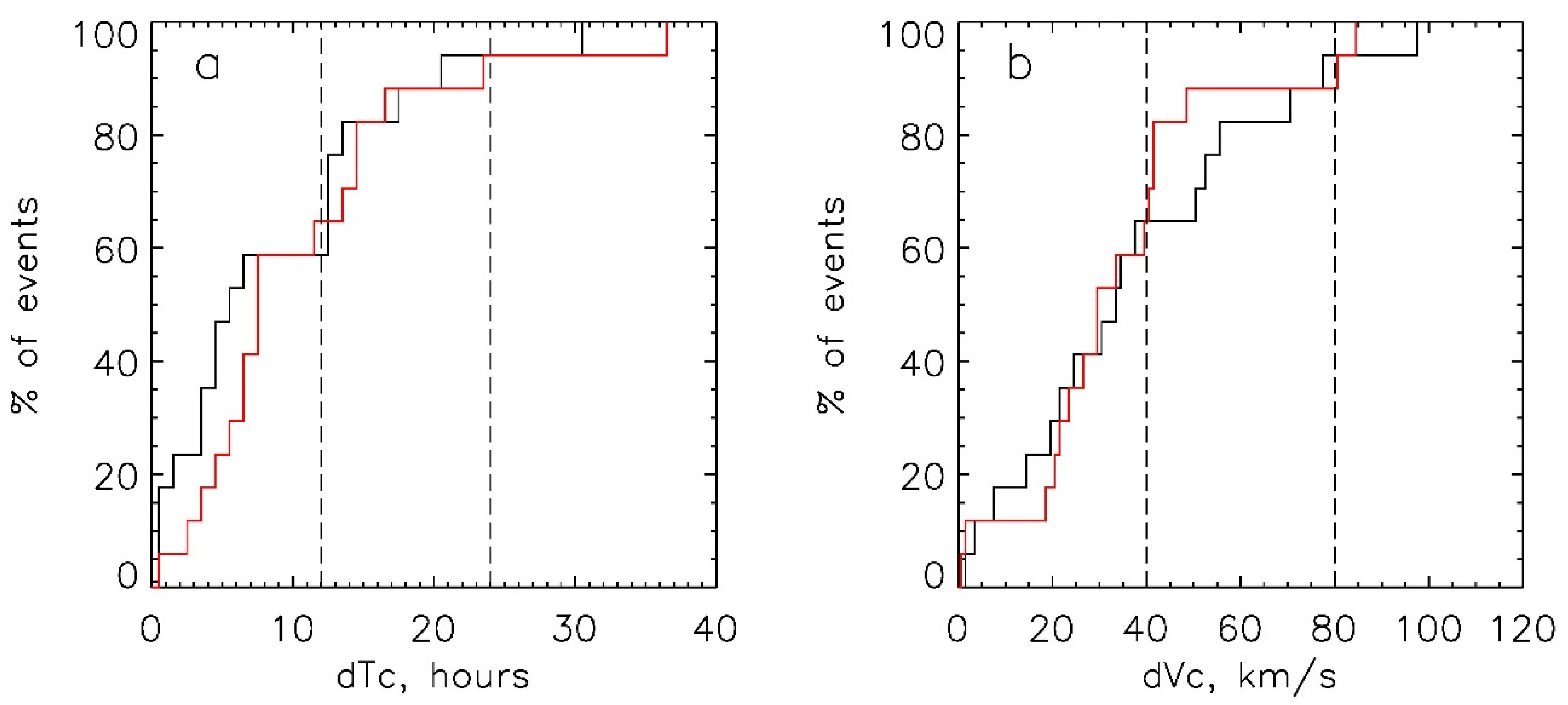
3.2. Optimization of the Prediction Algorithm and Estimation of the Confidence Intervals

After analysis of the SMDC testing results, we carried out ensemble simulations using a similar prediction algorithm in order to minimize errors and estimate the probabilities of successfully forecasted (hit) events within different confidence intervals. For simulation, we selected 17 ICMEs from the R&C list in the period 2013–2015 (

Table 5. Identification of solar origins for the selected ICMEs in the period 2013–2015 by RDBM.

#	Tstart_ICME, UT (R&C)	TR0, UT (γ = 0.2 × 10−7 km−1)	Tdimm,UT (Solar Demon)	Idimm × 105, DN s−1	Lat, deg	Lon, deg
1	2013-03-17 15:00	2013-03-15 15:48	2013-03-15 06:04	−1.26	8	−8
2	2013-04-14 17:00	2013-04-10 04:30	2013-04-11 07:00	−10.43	6	−16
3	2013-07-13 05:00	2013-07-09 03:19	2013-07-09 14:08	−6.97	17	−10
4	2013-08-23 20:00	2013-08-19 20:22	2013-08-21 03:22	−7.37	−16	−10
5	2013-10-02 23:00	2013-09-29 04:13	2013-09-29 21:22	−6.70	14	33
6	2014-02-16 05:00	2014-02-11 06:46	2014-02-12 04:24	−2.87	−13	7
7	2014-02-17 03:00	2014-02-12 12:55	2014-02-12 12:04	−8.42	5	25
8	2014-02-21 02:00	2014-02-17 18:22	2014-02-18 00:44	−7.89	−25	−31
9	2014-04-21 07:00	2014-04-18 10:45	2014-04-18 12:46	−6.51	−21	35
10	2014-09-12 22:00	2014-09-10 16:13	2014-09-10 17:26	−12.94	16	−3
11	2015-03-17 13:00	2015-03-14 21:28	2015-03-15 00:48	−8.53	−22	33
12	2015-04-10 13:00	2015-04-05 07:39	2015-04-06 18:42	−4.93	−15	−12
13	2015-06-23 02:00	2015-06-20 07:42	2015-06-21 01:40	−10.29	17	−16
14	2015-06-25 10:00	2015-06-22 12:04	2015-06-22 18:06	−5.48	17	7
15	2015-08-15 21:00	2015-08-12 03:40	2015-08-12 14:08	−2.63	−20	31
16	2015-11-07 06:00	2015-11-04 05:11	2015-11-04 13:42	−6.55	10	2
17	2015-12-20 03:00	2015-12-15 09:49	2015-12-16 08:04	−8.87	−12	1

T_{start_ICME}—the start time of the selected ICME from the R&C catalog; T_dimm, I_dimm, Lat, Lon—start time, lowest intensity and Stonyhurst central coordinates of the dimmings indicated in the Solar Demon database.

). The criteria for this selection were: appearance of evident dimmings and the indication of the associated CMEs in both the CACTus and CDAW CME databases. Some of the selected events are partly coincide with the SMDC test events for 2015, but their processing was completely independent including the determination of the CME solar sources.

Based on our own experience and the results of the CME predictions by other models [49,65,66,67,68,69], we propose that the errors in the arrival speed and time predicted by DBM are more critically defined by the accuracy of the difference between the CME speed and speed of the ambient SW (dV = V_CME -w) along the way from the Sun to the Earth, rather than by the uncertainties in other input data as the CME start time and γ; it follows from the quadratic dependence of the drag acceleration on dV, whereas the dependence on other parameters is linear. Furthermore, most of the prediction models consider CMEs as isolated structures, for which the drag force depends mainly on their geometrical shape [67] or variation of γ in the lower corona [70]. However, it was found in [71] that the population of single CMEs in 2010–2011 constitutes only about 52% of all events, the remaining 48% of CMEs interact with other SW streams in the heliosphere. In any case, CMEs interact with the ambient QSW, whose speeds may vary along the path from the Sun to the Earth. In the optimization procedure, we used the SINP QSW model, which enables the simulation of speed of the ambient SW along the heliosphere at any given time. Optimization of the drag parameter is more difficult, because it depends on the interaction between the CME plasma with the ambient SW (or other CMEs) in the heliosphere, so cannot be exactly known ahead. Therefore, we used the ensemble of simulations with variable values of γ and the modeled QSW speed with correction coefficients adjusted to obtain the minimum prediction errors.

To identify solar sources of the selected ICMEs, we tracked the ICMEs from the Earth back to the Sun using DBM in the reverse order (the RDBM procedure). The whole propagation range was divided into 4 subsequent spatial intervals in the reverse order (215–165 R_Sun, 165–115 R_Sun, 115–65 R_Sun, 65–20 R_Sun), and for each of them the arrival and departure times and speeds of the CME flows were calculated using the DBM equation, taking the drag acceleration term with the opposite sign. We calculated the ambient SW speed values on these spatial intervals calculated from the QSW modeled data (the SMDC website presents only the modeled speeds for 1 AU). It was found that the best agreement in time between the modeled and measured ICME parameters was achieved by using the QSW modeled speed with the correction coefficient 0.9, and by cutting its minimum value to 350 km s⁻¹. It corresponds to the best agreement between the modeled QSW speed and the measured SW speed in the slow SW according to the SRI catalog and the ACE data. The drag parameter was taken equal to γ = 0.2 × 10⁻⁷ km⁻¹. As a result, we obtained the supposed time (T_R20) and speed (V_R20) of the CMEs at a distance of 20 R_Sun (hereafter R₂₀) from the solar surface, which then were extrapolated to the solar surface (T_R0, V_R0 at R₀) by taking the average speed equal to V_R20/2 (in assumption of uniform acceleration of the CME plasma between R₀ and R₂₀).

We determined the sources of eruption by dimmings closest in time from the Solar Demon database, using that the dimming start time should be nearest in time to T₀ and its center was closest to the disk center as criteria. The centers of the found dimmings were positioned within −25° to 17° in latitude and −31° to 35° in longitude, with the lowest intensity in the dimming regions being from −1.24 × 10⁵ to −12.9 × 10⁵ DN s⁻¹. The corresponding CMEs were present in the CDAW and CACTus catalogs; their first appearance times differed from the dimming start time by less than 2 h. Parameters of the solar sources for the selected ICMEs are shown in Table 5.

At the second step, we calculated the predicted arrival time and speed of ICME to the Earth by the direct DBM in 4 spatial segments using the CACTus and CDAW times and speeds extrapolated to R₂₀ (see T₂₀, V₂₀ in

Table 6. Parameters of the CME sources identified from the CACTus and CDAW databases.

#	TR20, UT	VR20, km s−1	T20_CDAW, UT	V20_CDAW km s−1	T20_CACTus, UT	V20_CACTus km s−1
1	2013-03-15 01:20	811	2013-03-15 10:06	1161	2013-03-15 10:14	1016
2	2013-04-10 22:30	429	2013-04-11 10:59	819	2013-04-11 11:25	809
3	2013-07-09 18:44	502	2013-07-09 22:05	290	2013-07-09 23:17	392
4	2013-08-20 12:32	478	2013-08-21 13:14	321	2013-08-21 11:01	513
5	2013-09-29 18:45	532	2013-09-30 00:53	1164	2013-09-30 02:26	767
6	2014-02-12 02:43	388	2014-02-12 14:17	494	2014-02-12 13:13	441
7	2014-02-13 07:08	424	2014-02-12 19:00	492	2014-02-12 17:08	653
8	2014-02-18 05:37	687	2014-02-18 05:34	712	2014-02-18 04:56	926
9	2014-04-18 19:55	844	2014-04-18 15:59	1245	2014-04-18 16:16	1080
10	2014-09-10 22:12	1290	2014-09-10 20:26	1119	2014-09-10 20:54	994
11	2015-03-15 05:44	935	2015-03-15 06:06	682	2015-03-15 05:20	982
12	2015-04-06 05:39	351	2015-04-07 02:50	450	2015-04-07 01:55	474
13	2015-06-20 17:51	761	2015-06-21 04:51	1434	2015-06-21 05:12	1190
14	2015-06-22 21:42	804	2015-06-22 21:09	1147	2015-06-22 21:44	982
15	2015-08-12 18:39	516	2015-08-12 19:35	687	2015-08-12 20:09	624
16	2015-11-04 14:48	803	2015-11-04 20:09	701	2015-11-04 19:08	652
17	2015-12-16 05:02	402	2015-12-16 14:56	487	2015-12-16 13:43	716

T_{20_CACTUS}, V_{20_CACTUS}, T_{20_CDAW}, V_{20_CDAW} -times and speeds extrapolated from the CDAW and CACTus data; T_R20, V_R20—those obtained by RDBM. All times in hours, speeds—in km/s.

) as the initial data for the first segment. For other segments, we used as the initial data the departure time and speed of the previous segment.

To determine the optimal γ-value, we fulfilled calculations with γ changing from 0 to 1 × 10⁻⁷ km⁻¹ in 0.05 × 10⁻⁷ steps. Thus, for each γ-value we obtained the modeled arrival times and speeds for all selected ICMEs, which then we compared with the start time and average speed of the primary ICMEs indicated in the R&C list. Figure 4 shows the dependence of averaged (over all set of ICMEs) mean difference in time (dT) and speed (dV) between the modeled and measured values as a function of γ.

As a result, we determined that in both cases of the CACTus and CDAW initial data, the minimum differences dT, dV correspond to γ = 0.3 × 10⁻⁷ km⁻¹ which can be regarded as the optimal value for the given set of ICMEs. The same value was found in [68] using the Probabilistic Drag-Based Ensemble Model (DBEM), where the stochastic ensemble approach was applied for 146 ICME events from the R&C list (1996–2015).

Table 7. Prediction errors ME, MAE and SD for the tested ICME set obtained with the ensemble SMDC using the CACtus and CDAW data and γ_opt = 0.3 × 10⁻⁷ km⁻¹ in comparison with the “Average of all methods” Scoreboard data (see Table 3 from [65]) and with basic SMDC.

Data Parameter	CACTus		CDAW		Scoreboard		Basic SMDC (2015)
	Value	SD	Value	SD	Value	SD	Value	SD
ME(dT), h	−0.09	12.4	1.6	14.1	−3.67	17.1	2.7	26.8
MAE(dT), h	8.8	8.4	10.7	8.9	12.9	-	20.8	25.6
ME(dV), km s−1	0.94	47.2	0.35	41.8	-	-	6.2	101.6
MAE(dV), km s−1	37.5	27.0	34.2	22.5	-	-	82.3	100.1

shows the calculated with γ = γ_opt values of the prediction errors ME and MAE (mean absolute error) for the modeled with the ensemble SMDC arrival time dT and speed dV averaged over the studied set of the events (hits) with the corresponding standard deviations (SD).

The comparison of these results with those presented in the Scoreboard “Average of all methods” (Table 3 from [65]) shows that the ensemble SMDC model provides a prediction of the arrival time of the hit events with accuracy at the level, or even better than, the “Average of all models” errors presented in the Scoreboard (the errors in speed are not evaluated in Scoreboard). The accuracy of the ensemble SMDC in the ICME arrival speed (ME(dV) and MAE(dV) values in Table 7) are sufficiently better than that found in [68] with the DBEM v3 model: ME = 79.7 km s⁻¹, MAE = 131.2 km s⁻¹.

In order to estimate probabilities and confidence intervals of successful forecast (hits), we analyzed the spreads of absolute values of dT and dV for all selected ICMEs obtained with the ensemble SMDC model using the optimal γ value. The results are presented in Figure 5 and in

Table 8. Probabilities of the ICME forecast in % within the defined confidence intervals of arrival time dT_c and speed dV_c for the set of events of 2013–2015 obtained with the ensemble model for the CACTus and CDAW initial data and γ = 0.3 × 10⁻⁷ km⁻¹.

Confidence Intervals	dTc, Hours		dVc, km s−1
	<12	<24	<40	<80
CACTus	59	94	65	94
CDAW	65	94	65	88

. According to the Student’s t-distribution, the confidence level of our results obtained on 17 events is 0.95.

4. Discussion

According to Table 2, from 2015 to 2017 the numbers of hit and false alarm events decreased, while the number of the miss events increased. The values in brackets also show this (however, the difference between 2016 and 2017 is due to the small number of events which, reduces the significance of averaging). This effect may be described by the ratio between the number of the predicted events and the number of the events indicated in the ICME merged base. This value is called a “bias score”, where a bias score greater than 1 means a tendency to over-forecast, and the opposite situation means a tendency to under-forecast the prediction. The bias score obtained from Table 2 changes from 1.82 for 2015 to 0.61 for 2016, and finally to the value of 0.45 for 2017. This means that while the number of indicated near the Earth ICMEs decreases gradually, the number of CME sources that satisfied our selection algorithm drops sharply along with the decline in the solar activity. We could relate this to the Step 3 in our algorithm. The number of detected dimming decreases drastically in 2016 and 2017, as do the number of CMEs satisfied the Step 3 requirements. There were several months when only one or two dimmings were detected (December 2016, February 2017, March and May 2017, December 2017). As a result, the ratio of the final number of events after Step 4 to that of the initial CACTus is larger in 2015 (≈ 5%) compared to subsequent years (≈ 2%), and this affects the quality of the forecast. It leads us to the suggestion that we should use different selection steps for the different phases of the solar activity cycle. Near the maximum phase of the solar cycle, we can add more selection steps based on the CACTus and Solar Demon data such as dimming size, intensity, location, CME duration etc., in order to decrease the number of false alarms. At the same time, we can remove some selection steps for the solar minimum and decrease the number of misses. From all of the above, it follows that modifying the parameters of the selection algorithm for different periods is the one possible way to improve the forecast results.

There are several reasons that could explain the increase in the number of false alarms and misses. While comparing our results with the CCMC “Average all methods” we discovered that there are events that were presented in both predictions, but were not indicated in the ICME catalogs. On the other hand, there were events that could not be predicted by any model presented in the Scoreboard. That means that the causes of such false alarms and misses are not in our selection algorithm, but are more likely connected with the physical processes that govern the CME propagation through the heliosphere. For example, there was an event observed with LASCO coronagraphs on 9 November 2015 at 14:00 UT. We predicted this event, and so did three different scientific teams (Goddard Space Flight Center, Greenbelt, USA; Met Office, Exeter, UK; NSSC CAS, Beijing, China), according to the Scoreboard. However, that CME was not detected at the Earth.

The theory of CME deflection was well developed in [72,73]. The main idea of this theory is that a CME that moves slower than the background SW is deflected to the west. In contrast, when a CME moves faster than the background SW, the CME is deflected to the east. In fact, the DBM model takes into account the influence of the background solar wind, but does not consider that the background SW moves not radially, but along the Parker spiral, so it must not only accelerate or decelerate the CME but also deflect it. However, the research in [74] shows that this effect may not occur when we simulate the CME shock propagation. In [75], the system (iCAF) that takes into account deflection effect was proposed. It shows that taking the deflection phenomenon into account improves the success rate (the hits to observed ratio) by 19 percent. Currently, the SMDC system uses DBM in one-dimensional mode, but we plan to incorporate the deflection theory in the future. In addition, by the ensemble modeling it was shown that application of the correcting coefficients to the modeled QSW speed and optimization of γ may noticeably improve the prediction accuracy.

Another possible origin of the false alarms and miss events can be a type of CME interaction in the solar corona that changes the direction of the CME propagation. Gopalswamy et al. [76] analyzed the influence of coronal holes on the CME propagation and showed that open magnetic field lines from coronal holes cause CMEs to move away from their initial direction and deflect from the radial propagation. This effect is more pronounced in the solar activity declining phase, but also could be observed during the solar minimum and the rising phase. The following articles [77,78] describe different cases of the CME deflection caused by the background magnetic field.

The multi-CME events represent a more complicated case to forecast. The CME-CME interaction may influence forecast accuracy and lead to unexpectedly high geo-effectiveness of the event [71,79]. For example, in 2017 there were events with a CME-CME interaction which occurred in September. There was one event on the fourth of September and three events on the sixth of September that we revealed after applying the selection algorithm. In the present research, we do not take into account the CME-CME interaction effect on the CME arrival time and speed forecast, but in the future, it is possible with DBM model by using the speed of the previous CME as a background SW speed for the following CME. Werner et al. [80] used the MHD simulation for this event, and Scolini et al. [81] analyzed the geo-effectiveness of such structures.

Finally, we want to address one more cause for misses which is connected to the question: how do we determine that plasma parameters at the Earth’s orbit are related to ICME plasma? Each ICME database or catalog uses its own criteria for such determination. There are papers that have shown that some ICMEs were detected at the Earth’s orbit, but they did not list in catalogs because they do not meet the criteria [61,82]. Such events are not very geo-effective or powerful, but we should take them into account to properly evaluate our forecast methods.

According to the validation results, the most accurate forecasts with the DBM-based model (minimum dT and dV for appropriate γ) are achieved if the relative difference between the CME and ambient SW speeds at the starting point R₂₀ (|V₂₀-w|/w) is larger than 1. In this case, when this value is much less than 1, that is V₂₀ ~ w, the drag force becomes insignificant, and the expected time of arrival weakly depends on the γ-value. Such a situation is typical for the solar minimum, when the CME speed is low, so even small inaccuracies in the speed of a CME or background SW can cause large changes in the calculated arrival time. These cases, when the initial CME speed is less than the ambient SW speed, most likely need special consideration.

Comparing the results of the basic SMDC presented in Section 3.1 with that of the optimized ensemble version (Section 3.2) shows that the optimization of the background SW speed and the γ-value can sufficiently increase the accuracies of the arrival time and speed of ICMEs. The ensemble approach was successfully tested on the selected set of events and can be applied to improve uncertainties in the operational mode of forecasts. For this, if a new CME is identified after the initial filtering, the ensemble procedure should be processed on a sliding set of 10–15 previously positively forecasted (hit) CMEs. As a result, the optimal values of γ and the correction coefficients for the QSW speed will be defined, so the system will be adjusted to the current conditions of solar activity. The new forecast of the ICME arrival will be carried out with optimized parameters, and its accuracy will be defined by probabilities within the updated confidence intervals.

5. Conclusions

In this work we considered the main principles of operation of the SMDC online prediction system based on the data of available solar catalogs. The basic version of SMDC was tested on the ICME events of 2015–2017. We studied the possibilities to optimize predictions given by the system using the ensemble approach for the data from 2013–2015. The tests showed that the optimized SMDC system is able to provide a prediction of the ICME arrival to the Earth with high probability within the confidence intervals at the level of the best ICME forecasting models. The combination of the basic SMDC with the ensemble preprocessing of the previous events enables improved accuracy of predictions in the varying conditions of the solar activity.

References

1. Gringauz, K.I. Some results of experiments in interplanetary space by means of charged particle traps on Soviet space probes. In Proceedings of the Second International Space Science Symposium, Florence, Italy, 10–14 April 1961. [Google Scholar]
2. Neugebauer, M.; Snyder, C.W. Solar Plasma Experiment. Science 1962, 138, 1095–1097. [Google Scholar] [CrossRef]
3. Richardson, I.G.; Cane, H.V. Near-earth solar wind flows and related geomagnetic activity during more than four solar cycles (1963–2011). J. Space Weather Space Clim. 2012, 2, A02. [Google Scholar] [CrossRef] [Green Version]
4. Yermolaev, Y.I.; Nikolaeva, N.S.; Lodkina, I.G.; Yermolaev, M.Y. Large-scale solar wind structures: Occurrence rate and geoeffectiveness. In Proceedings of the 12th International Solar Wind Conference, Saint-Malo, France, 21–26 June 2009. [Google Scholar] [CrossRef] [Green Version]
5. Richardson, I.G.; Cliver, E.W.; Cane, H.V. Sources of geomagnetic activity over the solar cycle: Relative importance of CMEs, high-speed streams, and slow solar wind. J. Geophys. Res. 2000, 105, 18203–18213. [Google Scholar] [CrossRef]
6. Rust, D.M.; Hildner, E. Expansion of an X-ray coronal arch into the outer corona. Sol. Phys. 1976, 48, 381–387. [Google Scholar] [CrossRef]
7. Hudson, H.S.; Lemen, J.R.; St. Cyr, O.C.; Sterling, A.C.; Webb, D.F. X-ray coronal changes during Halo CMEs. Geophys. Res. Lett. 1998, 25, 2481–2484. [Google Scholar] [CrossRef] [Green Version]
8. Harrison, R.A.; Bryans, P.; Simnett, G.M.; Lyons, M. Coronal dimming and the coronal mass ejection onset. Astron. Astrophys. 2003, 400, 1071–1083. [Google Scholar] [CrossRef]
9. Zhang, J.; Dere, K.P.; Howard, R.A.; Bothmer, V. Identification of Solar Sources of Major Geomagnetic Storms between 1996 and 2000. Astrophys. J. 2003, 582, 520–533. [Google Scholar] [CrossRef]
10. Watari, S. Geomagnetic storms of cycle 24 and their solar sources. Earth Planets Space 2017, 69, 70. [Google Scholar] [CrossRef]
11. Syed Ibrahim, M.; Joshi, B.; Cho, K.S.; Kim, R.-S.; Moon, Y.-J. Interplanetary Coronal Mass Ejec-tions During Solar Cycles 23 and 24: Sun–Earth Propagation Characteristics and Consequences at the Near-Earth Region. Sol. Phys. 2019, 294, 54. [Google Scholar] [CrossRef]
12. Plunkett, S.P.; Singh, A.K. Coronal Mass Ejections (CMEs) and their geoeffectiveness during Solar Cycles 23 and 24: A comparative analysis of observational properties. Int. J. Emerg. Technol. Innov. Res. 2021, 8, b123–b137. [Google Scholar]
13. Scolini, C.; Messerotti, M.; Poedts, S.; Rodriguez, L. Halo coronal mass ejections during Solar Cycle 24: Reconstruction of the global scenario and geoeffectiveness. J. Space Weather Space Clim. 2018, 8, A09. [Google Scholar] [CrossRef] [Green Version]
14. Gopalswamy, N.; Yashiro, S.; Akiyama, S.; Xie, H. Estimation of Reconnection Flux Using Post-eruption Arcades and Its Relevance to Magnetic Clouds at 1 AU. Sol. Phys. 2017, 292, 65. [Google Scholar] [CrossRef] [Green Version]
15. Chertok, I.M.; Grechnev, V.V.; Abunin, A.A. An early diagnostics of the geoeffectiveness of solar eruptions from photospheric magnetic flux observations: The transition from SOHO to SDO. Sol. Phys. 2017, 292, 62. [Google Scholar] [CrossRef] [Green Version]
16. Grechnev, V.V.; Kochanov, A.A.; Uralov, A.M.; Slemzin, V.A.; Rodkin, D.G.; Goryaev, F.F.; Kiselev, V.I.; Myshyakov, I.I. Development of a Fast CME and Properties of a Related Interplanetary Transient. Sol. Phys. 2019, 294, 139. [Google Scholar] [CrossRef]
17. Lynch, B.J.; Al-Haddad, N.; Yu, W.; Palmerio, E.; Lugaz, N. On the utility of flux rope models for CME magnetic structure below 30R. Adv. Space Res. 2022, 70, 1614–1640. [Google Scholar] [CrossRef]
18. Arge, C.N.; Pizzo, V.J. Improvement in the prediction of solar wind conditions using near-real time solar magnetic field updates. J. Geophys. Res. 2000, 105, 10465–10479. [Google Scholar] [CrossRef]
19. Wang, Y.-M.; Sheeley, N.R., Jr. Solar wind speed and coronal flux-tube expansion. Astrophys. J. 1990, 355, 726–732. [Google Scholar] [CrossRef]
20. Nolte, J.T.; Krieger, A.S.; Timothy, A.F.; Gold, R.E.; Roelof, E.C.; Vaiana, G.; Lazarus, A.J.; Sullivan, J.D.; McIntosh, P.S. Coronal holes as source of solar wind. Sol. Phys. 1976, 46, 303–322. [Google Scholar] [CrossRef]
21. Bu, X.; Luo, B.; Shen, C.; Liu, S.; Gong, J.; Cao, Y.; Wang, H. Forecasting high-speed solar wind streams based on solar extreme ultraviolet images. Space Weather 2019, 17, 1040–1058. [Google Scholar] [CrossRef]
22. Rotter, T.; Veronig, A.M.; Temmer, M.; Vršnak, B. Real-time solar wind prediction based on SDO/AIA coronal hole data. Sol. Phys. 2015, 290, 1355–1370. [Google Scholar] [CrossRef]
23. Shugay, Y.; Slemzin, V.; Rodkin, D.; Yermolaev, Y.; Veselovsky, I. Influence of coronal mass ejections on parameters of high-speed solar wind: A case study. J. Space Weather Space Clim. 2018, 8, A28. [Google Scholar] [CrossRef]
24. Vršnak, B.; Temmer, M.; Veronig, A.M. Coronal holes and solar wind high-speed streams: I. forecasting the solar wind parame-ters. Sol. Phys. 2007, 240, 315–330. [Google Scholar] [CrossRef]
25. Owens, M.J.; Challen, R.; Methven, J.; Henley, E.; Jackson, D.R. A 27 day persistence model of near-Earth solar wind conditions: A long lead-time forecast and a benchmark for dynamical models. Space Weather 2013, 11, 225–236. [Google Scholar] [CrossRef]
26. Hudson, H.S.; Acton, L.W.; Freeland, S.L. A Long-Duration Solar Flare with Mass Ejection and Global Consequences. Astrophys. J. 1996, 470, 629. [Google Scholar] [CrossRef]
27. Webb, D.F.; Lepping, R.P.; Burlaga, L.F.; DeForest, C.E.; Larson, D.E.; Martin, S.F.; Plunkett, S.P.; Rust, D.M. The origin and development of the May 1997 magnetic cloud. J. Geophys. Res. Space Phys. 2000, 105, 27251–27259. [Google Scholar] [CrossRef]
28. Muhr, N.; Vršnak, B.; Temmer, M.; Veronig, A.M.; Magdalenić, J. ANALYSIS OF A GLOBAL MORETON WAVE OBSERVED ON 2003 OCTOBER 28. Astrophys. J. 2010, 708, 1639–1649. [Google Scholar] [CrossRef] [Green Version]
29. Attrill, G.D.R.; Harra, L.K.; van Driel-Gesztelyi, L.; Démoulin, P.; Wülser, J.-P. Coronal “wave”: A signature of the mechanism making CMEs largescale in the low corona? Astron. Nachr. 2007, 328, 760–763. [Google Scholar] [CrossRef]
30. Mandrini, C.H.; Nakwacki, M.S.; Attrill, G.; van Driel-Gesztelyi, L.; Démoulin, P.; Dasso, S.; Elliott, H. Are CME-Related Dimmings Always a Simple Signature of Interplanetary Magnetic Cloud Footpoints? Sol. Physics. 2007, 244, 25–43. [Google Scholar] [CrossRef]
31. Mason, J.P.; Woods, T.N.; Webb, D.F.; Thompson, B.J.; Colaninno, R.C.; Vourlidas, A. RELATIONSHIP OF EUV IRRADIANCE CORONAL DIMMING SLOPE AND DEPTH TO CORONAL MASS EJECTION SPEED AND MASS. Astrophys. J. 2016, 830, 20. [Google Scholar] [CrossRef] [Green Version]
32. Dissauer, K.; Veronig, A.M.; Temmer, M.; Podladchikova, T. Statistics of Coronal Dimmings Associated with Coronal Mass Ejections. II. Relationship between Coronal Dimmings and Their Associated CMEs. Astrophys. J. 2019, 874, 123. [Google Scholar] [CrossRef]
33. Jin, M.; Cheung, M.C.M.; DeRosa, M.L.; Nitta, N.V.; Schrijver, C.J. Coronal Mass Ejections and Dimmings: A Comparative Study Using MHD Simulations and SDO Observations. Astrophys. J. 2022, 928, 154. [Google Scholar] [CrossRef]
34. Kraaikamp, E.; Verbeeck, C. Solar Demon–an approach to detecting flares, dimmings, and EUV waves on SDO/AIA images. J. Space Weather Space Clim. 2015, 5, A18. [Google Scholar] [CrossRef] [Green Version]
35. St. Cyr, O.C.; Howard, R.A.; Sheeley, N.R.; Plunkett, S.P.; Michels, D.J.; Paswaters, S.E.; Koomen, M.J.; Simnett, G.M.; Thompson, B.J.; Gurman, J.B.; et al. Properties of coronal mass ejections: SOHO LASCO observations from January 1996 to June 1998. J. Geophys. Res. 2000, 105, 18169–18185. [Google Scholar] [CrossRef]
36. Andrews, M.D.; Howard, R.A. A two-type classification of LASCO coronal mass ejection. Space Sci. Rev. 2001, 95, 147–163. [Google Scholar] [CrossRef]
37. Shen, F.; Wu, S.T.; Feng, X.; Wu, C.-C. Acceleration and deceleration of coronal mass ejections during propagation and interaction. J. Geophys. Res. 2012, 117, A11101. [Google Scholar] [CrossRef] [Green Version]
38. Vourlidas, A.; Howard, R.A.; Esfandiari, E.; Patsourakos, S.; Yashiro, S.; Michalek, G. Comprehensive Analysis of Coronal Mass Ejection Mass and Energy Properties over A Full Solar Cycle. Astrophys. J. 2011, 722, 1522–1538. [Google Scholar] [CrossRef] [Green Version]
39. Gopalswamy, N.; Dal Lago, A.; Yashiro, S.; Akiyama, S. The Expansion and Radial Speeds of Coronal Mass Ejections. Cent. Eur. Astrophys. Bull. 2009, 33, 115–124. [Google Scholar]
40. Na, H.; Moon, Y.-J.; Lee, H. Development of a Full Ice-cream Cone Model for Halo Coronal Mass Ejections. Astrophys. J. 2017, 839, 82. [Google Scholar] [CrossRef]
41. Cargill, P.J.; Chen, J.; Spicer, D.S.; Zalesak, S.T. Magnetohydrodynamic simulations of the motion of magnetic flux tubes through a magnetized plasma. J. Geophys. Res. 1996, 101, 4855–4870. [Google Scholar] [CrossRef]
42. Cargill, P.J. On the aerodynamic drag force acting on interplanetary coronal mass ejections. Sol. Phys. 2004, 221, 135–149. [Google Scholar] [CrossRef]
43. Vršnak, B.; Žic, T.; Falkenberg, T.V.; Möstl, C.; Vennerstrom, S.; Vrbanec, D. The role of aerodynamic drag in propagation of interplanetary coronal mass ejections. Astron. Astrophys. 2010, 512, A43. [Google Scholar] [CrossRef]
44. Vršnak, B.; Žic, T.; Vrbanec, D.; Temmer, M.; Rollett, T.; Möstl, C.; Veronig, A.; Čalogović, J.; Dumbović, M.; Lulić, S.; et al. Propagation of interplanetary coronal mass ejections: The drag-based model. Sol. Phys. 2013, 285, 295–315. [Google Scholar] [CrossRef]
45. Vršnak, B.; Ruždjak, D.; Sudar, D.; Gopalswamy, N. Kinematics of coronal mass ejections between 2 and 30 solar radii. What can be learned about forces governing the eruption? Astron. Astrophys. 2004, 423, 717–728. [Google Scholar] [CrossRef]
46. Vršnak, B. Analytical and empirical modelling of the origin and heliospheric propagation of coronal mass ejections, and space weather applications. J. Space Weather Space Clim. 2021, 11, 34. [Google Scholar] [CrossRef]
47. Vourlidas, A.; Patsourakos, S.; Savani, N.P. Predicting the geoeffective properties of coronal mass ejections: Current status, open issues and path forward. Philos. Trans. R. Soc. A Math. Phys. Eng. Sci. 2019, 377, 20180096. [Google Scholar] [CrossRef]
48. Dumbovic, M.; Calogovic, J.; Martinic, K.; Vrsnak, B.; Sudar, D.; Temmer, M.; Veronig, A. Drag-based model (DBM) tools for forecast of coronal mass ejection arrival time and speed. Front. Astron. Space Sci. 2021, 8, 58. [Google Scholar] [CrossRef]
49. Žic, T.; Vršnak, B.; Temmer, M. Heliospheric propagation of coronal mass ejections: Drag-based model fitting. Astrophys. J. Suppl. Ser. 2015, 218, 32. [Google Scholar] [CrossRef] [Green Version]
50. Hinterreiter, J.; Amerstorfer, T.; Temmer, M.; Reiss, M.A.; Weiss, A.J.; Möstl, C.; Barnard, L.A.; Pomoell, J.; Bauer, M.; Amerstorfer, U.V. Drag-based CME modeling with heliospheric images incorporating frontal deformation: ELEvoHI 2.0. Space Weather 2021, 19, e2021SW002836. [Google Scholar] [CrossRef]
51. Napoletano, G.; Foldes, R.; Camporeale, E.; Gasperis, G.; Giovannelli, L.; Paouris, E.; Pietropaolo, E.; Teunissen, J.; Tiwari, A.K.; Del Moro, D. Parameter Distributions for the Drag-Based Modeling of CME Propagation. Space Weather 2022, 20, e2021SW002925. [Google Scholar] [CrossRef]
52. Rollett, T.; Möstl, C.; Isavnin, A.; Davies, J.A.; Kubicka, M.; Amerstorfer, U.V.; Harrison, R.A. ElEvoHI: A novel CME prediction tool for heliospheric imaging combining an elliptical front with drag-based model fitting. Astrophys. J. 2016, 824, 131. [Google Scholar] [CrossRef] [Green Version]
53. Yermolaev, Y.I.; Yermolaev, M.Y.; Lodkina, I.G.; Nikolaeva, N.S. Statistical Investigation of Heliospheric Conditions Resulting in Magnetic Storms. Cosm. Res. 2007, 45, 1–8. [Google Scholar] [CrossRef]
54. Lemen, J.R.; Title, A.M.; Akin, D.J.; Boerner, P.F.; Chou, C.; Drake, J.F.; Duncan, D.W.; Edwards, C.G.; Friedlaender, F.M.; Heyman, G.F.; et al. The Atmospheric Imaging Assembly (AIA) on the Solar Dynamics Observatory (SDO). Sol. Phys. 2012, 275, 17–40. [Google Scholar] [CrossRef] [Green Version]
55. Brueckner, G.E.; Howard, R.A.; Koomen, M.J.; Korendyke, C.M.; Michels, D.J.; Moses, J.D.; Socker, D.G.; Dere, K.P.; Lamy, P.L.; Llebaria, A.; et al. The Large Angle Spectroscopic Coronagraph (LASCO). Sol. Phys. 1995, 162, 357–402. [Google Scholar] [CrossRef]
56. Lamy, P.L.; Floyd, O.; Boclet, B.; Wojak, J.; Gilardy, H.; Barlyaeva, T. Coronal Mass Ejections over Solar Cycles 23 and 24. Space Science Rev. 2019, 215, 39. [Google Scholar] [CrossRef] [Green Version]
57. Richardson, I.G.; Cane, H.V. Near-Earth Interplanetary Coronal Mass Ejections During Solar Cycle 23 (1996–2009): Catalog and Summary of Properties. Sol. Phys. 2010, 264, 189–237. [Google Scholar] [CrossRef]
58. Stone, E.C.; Frandsen, A.M.; Mewaldt, R.A.; Christian, E.R.; Margolies, D.; Ormes, J.F.; Snow, F. The Advanced Composition Explorer. Space Sci. Rev. 1998, 86, 1–22. [Google Scholar] [CrossRef]
59. Yermolaev, Y.I.; Nikolaeva, N.S.; Lodkina, I.G.; Yermolaev, M.Y. Catalog of Large-Scale Solar Wind Phenomena during 1976-2000. Cosm. Res. 2009, 47, 81–94. [Google Scholar] [CrossRef]
60. Kaportseva, K.B.; Shugay, Y.S. Use of the DBM Model to the Predict of Arrival of Coronal Mass Ejections to the Earth. Cosm. Res. 2021, 59, 268–279. [Google Scholar] [CrossRef]
61. Kilpua, E.K.J.; Jian, L.K.; Li, Y.; Luhmann, J.G.; Russell, C.T. Observations of ICMEs and ICME-like Solar Wind Structures from 2007 – 2010 Using Near-Earth and STEREO Observations. Sol. Phys. 2012, 281, 391–409. [Google Scholar] [CrossRef]
62. Shugai, Y.S. Analysis of Quasistationary Solar Wind Stream Forecasts for 2010–2019. Russ. Meteorol. Hydrol. 2021, 46, 172–178. [Google Scholar] [CrossRef]
63. Kalegaev, V.; Panasyuk, M.; Myagkova, I.; Shugay, Y.; Vlasova, N.; Barinova, W.; Beresneva, E.; Bobrovnikov, S.; Eremeev, V.; Dolenko, S.; et al. Monitoring, analysis and post-casting of the Earth’s particle radiation environment during February 14–March 5, 2014. J. Space Weather Space Clim. 2019, 9, A29. [Google Scholar] [CrossRef]
64. Reiss, M.A.; Temmer, M.; Veronig, A.M.; Nikolic, L.; Vennerstrom, S.; Schöngassner, F.; Hofmeister, S.J. Verification of high-speed solar wind stream forecasts using operational solar wind models. Space Weather 2016, 14, 495–510. [Google Scholar] [CrossRef] [Green Version]
65. Riley, P.; Mays, M.L.; Andries, J.; Amerstorfer, T.; Biesecker, D.; Delouille, V.; Dumbović, M.; Feng, X.; Henley, E.; Linker, J.A.; et al. Forecasting the Arrival Time of Coronal Mass Ejections: Analysis of the CCMC CME Scoreboard. Space Weather 2018, 16, 1245–1260. [Google Scholar] [CrossRef] [Green Version]
66. Mays, M.L.; Taktakishvili, A.; Pulkkinen, A.; MacNeice, P.J.; Rastätter, L.; Odstrcil, D.; Jian, L.K.; Richardson, I.G.; LaSota, J.A.; Zheng, Y.; et al. Ensemble Modeling of CMEs Using the WSA–ENLIL+Cone Model. Sol. Phys. 2015, 290, 1775–1814. [Google Scholar] [CrossRef] [Green Version]
67. Dumbović, M.; Čalogović, J.; Vršnak, B.; Temmer, M.; May, M.L.; Veronig, A.; Piantschitsch, I. The Drag-based Ensemble Model (DBEM) for Coronal Mass Ejection Propagation. Astrophys. J. 2018, 854, 180. [Google Scholar] [CrossRef]
68. Čalogović, J.; Dumbović, M.; Sudar, D.; Vršnak, B.; Martinić, K.; Temmer, M.; Veronig, A. Probabilistic Drag-Based Ensemble Model (DBEM) Evaluation for Heliospheric Propagation of CMEs. Sol. Phys. 2021, 296, 114. [Google Scholar] [CrossRef]
69. Napoletano, G.; Forte, R.; Del Moro, D.; Pietropaolo, E.; Giovannelli, L.; Berrilli, F. A probabilistic approach to the drag-based model. J. Space Weather Space Clim. 2018, 8, A11. [Google Scholar] [CrossRef] [Green Version]
70. Hess, P.; Zhang, J. Stereoscopic study of the kinematic evolution of a coronal mass ejection and its driven shock from the sun to the earth and the prediction of their arrival times. Astrophys. J. 2014, 792, 49. [Google Scholar] [CrossRef]
71. Rodkin, D.; Slemzin, V.; Zhukov, A.N.; Goryaev, F.; Shugay, Y.; Veselovsky, I. Single ICMEs and Complex Transient Structures in the Solar Wind in 2010–2011. Sol. Phys. 2018, 293, 78. [Google Scholar] [CrossRef] [Green Version]
72. Wang, Y.; Shen, C.; Wang, S.; Ye, P. Deflection of coronal mass ejection in the interplanetary medium. Sol. Phys. 2004, 222, 329–343. [Google Scholar] [CrossRef]
73. Wang, Y.; Wang, B.; Shen, C.; Shen, F.; Lugaz, N. Deflected propagation of a coronal mass ejection from the corona to interplanetary space. J. Geophys. Res. Space Phys. 2014, 119, 5117–5132. [Google Scholar] [CrossRef]
74. Prise, A.J.; Harra, L.K.; Matthews, S.A.; Arridge, C.S.; Achilleos, N. Analysis of a coronal mass ejection and corotating interaction region as they travel from the Sun passing Venus, Earth, Mars, and Saturn. J. Geophys. Res. Space Phys. 2015, 120, 1566–1588. [Google Scholar] [CrossRef] [Green Version]
75. Zhuang, B.; Wang, Y.; Shen, C.; Liu, S.; Wang, J.; Pan, Z.; Li, H.; Liu, R. The Significance of the Influence of the CME Deflection in Interplanetary Space on the CME Arrival at Earth. Astrophys. J. 2017, 845, 117. [Google Scholar] [CrossRef]
76. Gopalswamy, N.; Mäkelä, P.; Xie, H.; Akiyama, S.; Yashiro, S. CME interactions with coronal holes and their interplanetary consequences. J. Geophys. Res. Space Phys. 2009, 114, A00A22. [Google Scholar] [CrossRef]
77. Sieyra, M.V.; Cécere, M.; Cremades, H.; Iglesias, F.A.; Sahade, A.; Mierla, M.; Stenborg, G.; Costa, A.; West, M.J.; D’Huys, E. Analysis of Large Deflections of Prominence–CME Events during the Rising Phase of Solar Cycle 24. Sol. Phys. 2020, 295, 126. [Google Scholar] [CrossRef]
78. Kilpua, E.K.J.; Pomoell, J.; Vourlidas, A.; Vainio, R.; Luhmann, J.; Li, Y.; Schroeder, P.; Galvin, A.B.; Simunac, K. STEREO observations of interplanetary coronal mass ejections and prominence deflection during solar minimum period. Ann. Geophys. 2009, 27, 4491–4503. [Google Scholar] [CrossRef] [Green Version]
79. Rodkin, D.; Kaportseva, K.B.; Lukashenko, A.T.; Veselovsky, I.S.; Slemzin, V.A.; Shugay, Y.S. Large-Scale and Small-Scale Solar Wind Structures Formed during Interaction of Streams in the Heliosphere. Cosm. Res. 2019, 57, 18–28. [Google Scholar] [CrossRef]
80. Werner, A.L.E.; Yordanova, E.; Dimmock, A.P.; Temmer, M. Modeling the Multiple CME Interaction Event on 6–9 September 2017 with WSA-ENLIL+Cone. Space Weather. 2019, 17, 357–369. [Google Scholar] [CrossRef]
81. Scolini, C.; Chané, E.; Temmer, M.; Kilpua, E.K.J.; Dissauer, K.; Veronig, A.M.; Palmerio, E.; Pomoell, J.; Dumbović, M.; Guo, J.; et al. CME–CME Interactions as Sources of CME Geoeffectiveness: The Formation of the Complex Ejecta and Intense Geomagnetic Storm in 2017 Early September. Astrophys. J. Suppl. Ser. 2020, 247, 21. [Google Scholar] [CrossRef]
82. Slemzin, V.; Goryaev, F.; Rodkin, D. Formation of Coronal Mass Ejection and Posteruption Flow of Solar Wind on 2010 August 18 Event. Astrophys. J. 2022, 929, 146. [Google Scholar] [CrossRef]
Figure 1. The picture represents measured (blue line) and on-line forecasted by the QSW model (red line) velocities of the SW at the L1 Sun-Earth point from page at the SINP MSU site (https://swx.sinp.msu.ru/weather.php?lang=en (accessed on 25 August 2022)).
Universe 08 00565 g001
Figure 2. Scheme of the basic SMDC forecasting system. V_CME and T_start are the CME parameters obtained from the CACTus database, Rs is the solar radius, R0 is the distance to which the DBM input parameters are recalculated. T0 and v0 are the CME parameters at 20Rs, w is the ambient SW speed, γ is a drag parameter.
Universe 08 00565 g002
Figure 3. Distributions of the ICME arrival time errors for the events of 2015–2017 predicted by SMDC (the white bars) and CCMC Scoreboard (the gray bars). The y-axis shows the percentage of the observed hit events depending on the time error within the interval in hours marked on the x-axis.
Universe 08 00565 g003
Figure 4. The time (dT) and speed (dV) difference between the modeled by the ensemble SMDC arrival times and speeds of the ICMEs and start times and averaged speeds in the R&C catalog as a function of γ for the CACTus (the black lines and symbols) and CDAW (the red lines and symbols) initial data. The dashed line corresponds to the optimal γ-value.
Universe 08 00565 g004
Figure 5. Probabilities of the ICME forecast obtained with the ensemble model for γopt = 0.3 × 10⁻⁷ km−1 as a function of the confidence intervals: (a) for the values |dT|dTc, (b) for |dV|dVc. The black lines correspond to the initial CACTus data, the red lines—to the CDAW data. The dashed lines show the limits of the confidence intervals according to Table 8.
Universe 08 00565 g005