About Cosmic Ray Modulation in the Heliosphere

Abstract

Cosmic ray fluxes in the heliosphere are modulated by solar wind with an embedded solar interplanetary magnetic field. The solar activity changes with a period of ~11 year, and this is the main reason for the observed 11-year variations of cosmic ray fluxes. Besides this, the directions of magnetic fields in solar polar regions and in the heliosphere change to the opposite direction every ~11-years. This causes, in addition, the presence of another 22-year solar magnetic cycle and contributes features to the known ~11-cycle. In this article, we discuss the generally accepted picture of cosmic ray modulation in the heliosphere and show that it requires several changes.

1. Introduction

Cosmic rays, which are charged particles (protons, nuclei, and very small part of electrons), come to us from the interstellar medium. To reach the Earth’s orbit or nearby space, these particles have to cross the heliosphere: the space around the Sun. The size (~radius) of this solar environment is more than 100 astronomical units (au). The heliosphere is filled with solar wind with a magnetic field frozen into it. In the solar wind, there always are magnetic inhomogeneities, scattering the charged particles [1]. Therefore, the cosmic ray (CR) fluxes in the heliosphere are always less than in outer space. The concentration of magnetic inhomogeneities in the heliosphere and, consequently, the amplitude of CR modulation is determined by the level of solar activity; for example, the number of sunspots.

Solar activity changes with a period of ~11 year. The sunspot number is used as a solar activity parameter that reflects the changes in the solar wind and interplanetary magnetic field. Thus, CRs undergo 11-year variations. Moreover, a quasi-regular solar magnetic field fills the heliosphere. The direction of the magnetic fields in the heliosphere are changed to opposite every ~11-years, and we have a 22-year solar magnetic cycle, together with an 11-year solar activity cycle.

In the heliosphere four physical mechanisms are responsible for CR modulation, namely: (1) diffusion of CRs from interstellar space into the heliosphere; (2) convection of particles from the heliosphere by solar wind with an embedded magnetic field; (3) adiabatic energy losses of charged particles in the expanding solar wind; and, finally, (4) the drift of cosmic rays in the quasi-regular solar magnetic field [1,2].

Among the four mechanisms mentioned above, the processes of diffusion, convection, and adiabatic energy losses of cosmic particles do not depend on the sign of particle electric charge. Only the drift effects of charged particles in quasi-regular heliospheric magnetic fields depend on the sign of the electric charge of particles. The directions of drift velocities of electrons and positrons, protons, and antiprotons are opposite. These directions will reverse every ~11 years, because the magnetic field directions in the heliosphere change with such a period.

It was discovered that the long-term variations of CR fluxes show peak-like and plateau-like forms of time dependences, in successive 11-cycles of solar activity. The generally accepted explanation for this phenomenon is the significant contribution of drift effects to the process of CR propagation in the heliosphere. From this point of view, if we observe a peak-like form for protons, we should observe a plateau-like form for electrons, and vice versa. However, the experimental data do not agree with this conclusion.

Below, we will discuss the processes of CR modulation in the heliosphere and show the generally accepted model of CR modulation requires significant changes.

2. Data on Cosmic Rays, and Solar and Heliospheric Magnetic Fields

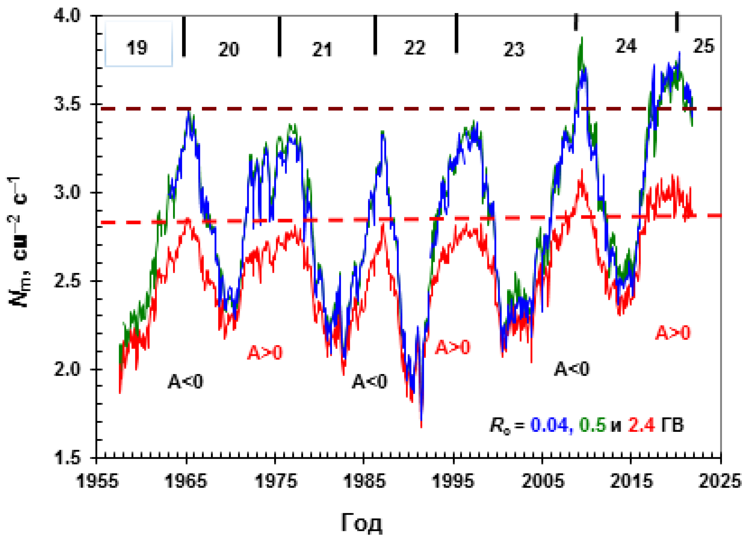
In Figure 1, the time dependences of CR fluxes, N_m, in the cascade curve maximum (Pfotzer–Regener maximum) in the Earth’s atmosphere are shown [3]. These particles are secondary ones. They are produced by primary CRs (protons and nuclei) falling on the top of the atmosphere and having rigidities R greater than the geomagnetic cutoff rigidity R_c. In Figure 1, the ~11-year cycle variation in CR fluxes is clearly visible.

The 11-year solar activity cycle is responsible for the corresponding changes of CR fluxes. After a minimum of solar activity with a delay of about one year, the maximum CR flux is observed. The amplitude of the 11-year variations of CRs decreases with the increase of particle energies or the geomagnetic cutoff rigidity, R_c. For example, using the data presented in Figure 1, one can compare CR fluxes in 1990 (max solar activity) and 1996 (min solar activity) obtained at the same latitude. The difference between the minimum and maximum values of N_m obtained at the polar latitudes with low R_c (green and blue curves in Figure 1) is larger than the difference between the corresponding values of N_m obtained at the middle latitude with R_c = 2.4 GV (red curve in Figure 1). In the solar cycles of 24 and 25, the minimum levels of solar activity were very low in comparison with the previous ones (19–23 solar cycles). In these cycles, a year after the solar activity minima, the maximum fluxes of CRs (~2009 and ~2021) were measured for the entire history of their observations.

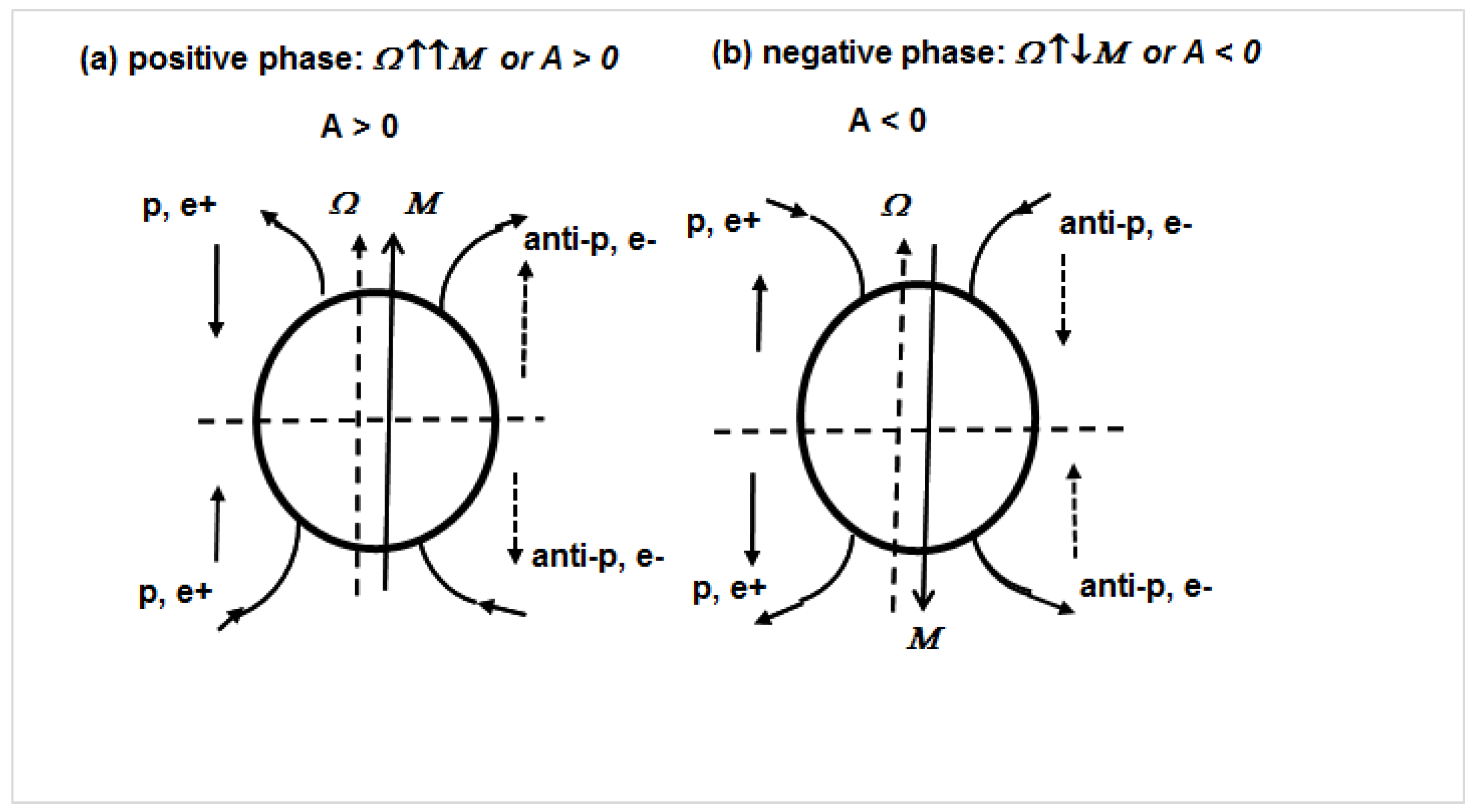
The time dependences of N_m show alternating shapes of peaked parts and plateau-like ones. The time interval between peaks or plateaus is ~22-years. This phenomenon is due to the 22-year solar magnetic cycle [4]. Roughly, we can consider the magnetic field of the Sun as a magnetic dipole, except for the three years of solar activity maximum, when inversion of the solar polar magnetic field occurs. This magnetic cycle has two phases: (1) a positive one, when the magnetic field lines come out of the northern polar cap of the Sun and enter the south polar cap. This is denoted as A > 0, or Ω ↑↑M, where Ω is the Sun’s angular velocity, M is the solar dipole magnetic moment; (2) a negative phase, when the magnetic field lines enter the north polar cap of the Sun and emerge from the south polar one. This is denoted as A < 0, or Ω ↑↓M. The solar wind stretches the solar magnetic field lines in the heliosphere at distances more than 100 au.

In the heliosphere, during each phase of the 22-year magnetic cycle, the directions of magnetic fields are preserved, and the directions of magnetic field lines are the same as in the solar polar caps, except for the period of the reversal of the solar magnetic field (or inversion period).

As will be shown below, the directions of magnetic field lines have a significant effect on the fluxes of CRs in the heliosphere [2,5]. As follows from Figure 1, the peaked time dependence of cosmic rays is observed in negative phases (A < 0) of the 22-year solar magnetic cycle and flatness is observed during positive ones (A > 0). The CR fluxes, as a rule, are higher in the negative phase in comparison with the positive one.

CRs in the heliosphere experience drift. There are two types of drifts: gradient drift with velocity

v_g = [(α²ω_B)/(2B²)]⋅[B × ∇B]

(1)

and centrifugal drift,

v_c ≈ (c·γ·m/q) (v_ǁ)²[r × B]/(R²B²)

(2)

where α—larmor radius of particle, B—induction of the interplanetary magnetic field (IMF), r—radius of curvature of the magnetic field line of IMF, q—electric charge of particle, m—mass of particle, c—speed of light, γ—Lorentz-factor, ω_B = |q|B/γmc_—cyclotron frequency in a magnetic field B [6,7]. The direction of a drift velocity depends on the sign of the electric charge of the particle. Consequently, in the heliosphere, the drift velocities of protons (positrons) and electrons will have opposite directions.

In Figure 2, the directions of the magnetic field on the Sun, in the heliosphere, and the directions of drift velocities for protons, positrons, antiprotons, and electrons are shown for positive (a) and negative (b) phases of the 22-year solar magnetic cycle.

Since the direction of the drift currents of particles is determined by the sign of their electric charge, it was naturally assumed that the drift of particles is responsible for the peak and plateau shapes of the time dependences observed in CRs. The direction of magnetic field lines and the sign of electric charge define the direction of drift velocity of a particle (expressions 1 and 2). Schematically, the time dependencies of CR fluxes (protons and electrons) are shown in Figure 3 for positive (A > 0) and negative (A < 0) phases of the 22-year solar magnetic cycle.

According to the modern theoretical concept, and as is seen from Figure 3, the flux of CRs with a positive electric charge (black curve) have their peak during the solar activity minimum if we are in the negative phase of the 22-year solar magnetic cycle (A < 0). In the positive phase of cycle (A > 0), for positive charged particles, a plateau is observed. For particles with a negative electric charge, the opposite picture is observed (red curve).

Let us do an analysis of the experimental data and compare them with the theoretical concepts.

3. Comparison of Experimental Data and Theory

To date, quite a lot of experimental data have been obtained on electrons in CRs over a long time interval. We can compare the time dependences of electrons and protons.

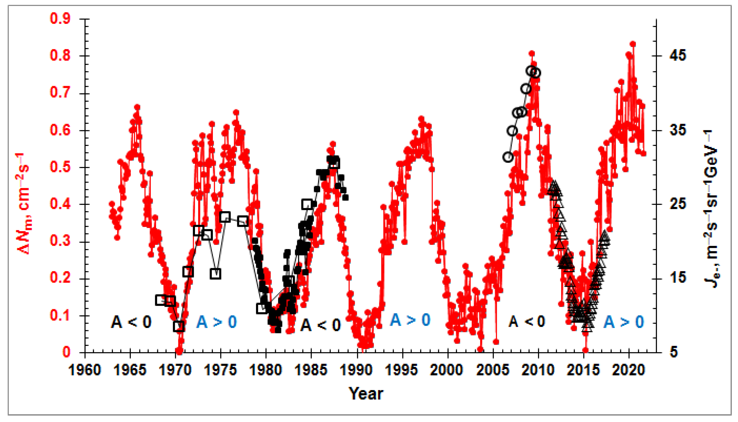
Figure 4 shows the time dependence of secondary CR fluxes measured in the Pfotzer–Regener maximum in the Earth’s atmosphere, ΔN_m [3]. These secondary particles were produced by primary protons and nuclei with the rigidities R = 0.73–2.4 GV (protons with energies E = 250–1500 MeV). The values of ΔN_m were obtained from the data presented in Figure 1 as the differences between the values of N_m measured at the latitudes with geomagnetic cutoff rigidities of R_c = 0.5 and 2.4 GV. In addition, Figure 4 presents the intensities of electrons. The amplitudes of time variations of secondary particles in the Earth’s atmosphere, produced by primary protons and nuclei, and the amplitudes of time variations of primary electrons are comparable to each other.

As one can see from Figure 4, in the period 1974–1978, a plateau-like time dependence was observed in cosmic rays produced by primary protons and nuclei (red curve). This plateau-like time dependence was also seen for electrons. In the periods of 1983–1988 and 2007–2012, peak-like time dependences were observed, both for particles with positive and negative electric charges. These results contradict modern theoretical ideas about CR modulation in the heliosphere and contradict the conclusion given in [10].

Thus, from the data given in Figure 4, one can conclude that the drifts of particles with positive and negative electric charges cannot be responsible for the appearance of peak-like and plateau-like time dependences in CRs. We can simultaneously observe peak-like or plateau-like time dependences for particles with positive and negative electric charges [11].

4. Modulation of Electrons and Positrons. High-Energy Cosmic Rays

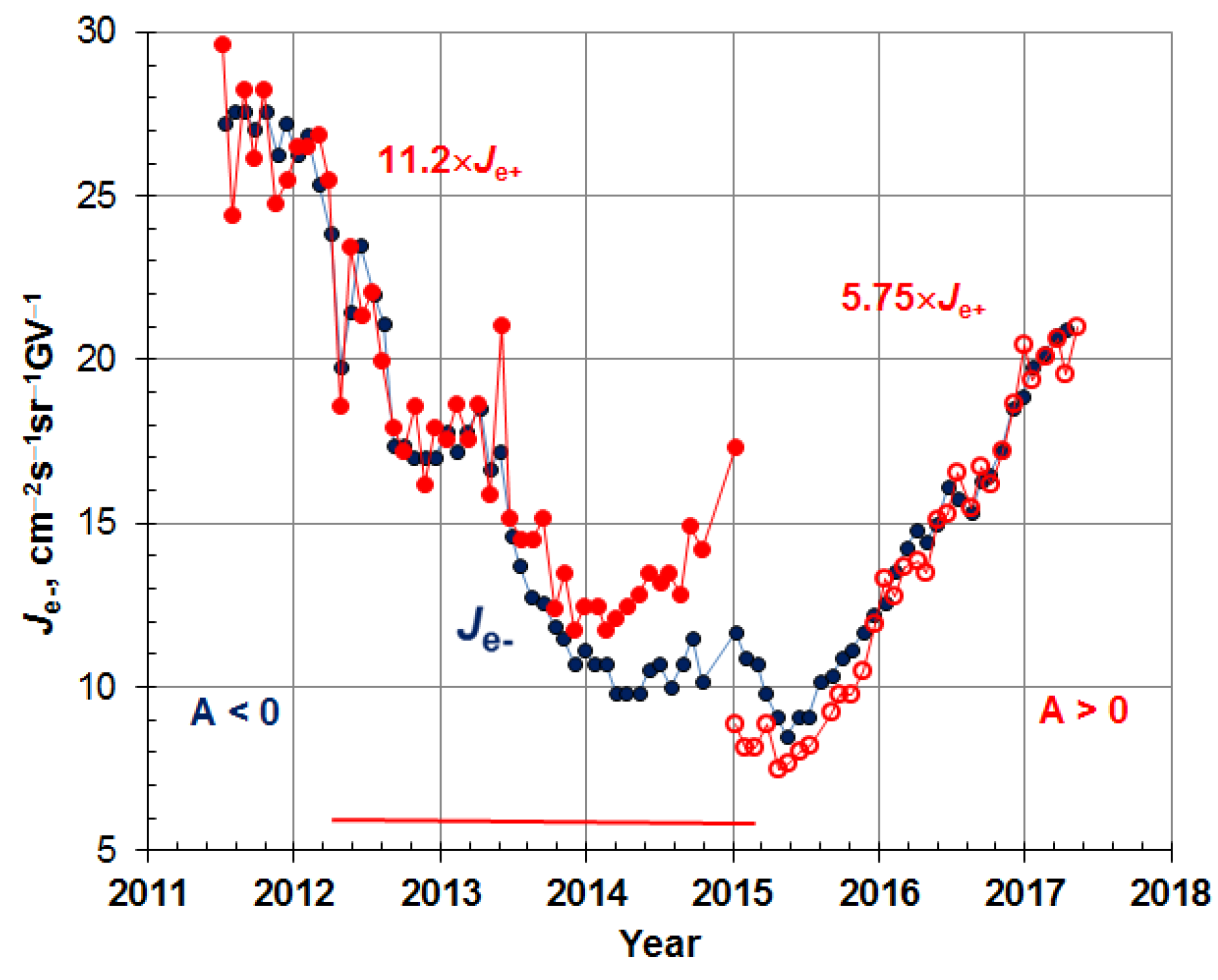
In space experiments, the PAMELA and AMS-02 magnetic spectrometers have measured the primary fluxes of electrons and positrons. Therefore, there is a possibility to study the modulation processes of these particles in the 11- and 22-year solar cycles. For analysis, as an example, we choose the electron and positron intensities with rigidities R = 1.0–1.2 GV [9]. The time dependences of these particle fluxes are depicted in Figure 5.

Figure 5 shows that the time changes of electron and positron intensities occurred in phase with each other in the periods from the middle of 2011 to the middle of 2013, and from the 2016 to the middle of 2017. The first period corresponds to the negative phase of the solar magnetic cycle (A < 0), and the second period corresponds to the positive one (A > 0).

The horizontal straight red line shows the beginning and the end of the inversion of polar solar magnetic field. The cosmic rays “feel” the rearrangement of the magnetic field in the heliosphere about a year after the beginning of this process on the Sun. The process of inversion of the magnetic field in the heliosphere ends about a year after the end of the process of inversion of the magnetic field on the Sun. It takes about one year for the solar wind to reach the heliopause.

During the inversion of magnetic fields on the Sun and in the heliosphere, the directions of drift currents are reversed. When A < 0, the drift current of electrons in the heliosphere is directed from high heliolatitudes to solar equatorial plane. The drift currents of positrons, protons, and nuclei are directed from solar equator toward high heliolatitudes. When A > 0, the situation changes to the opposite.

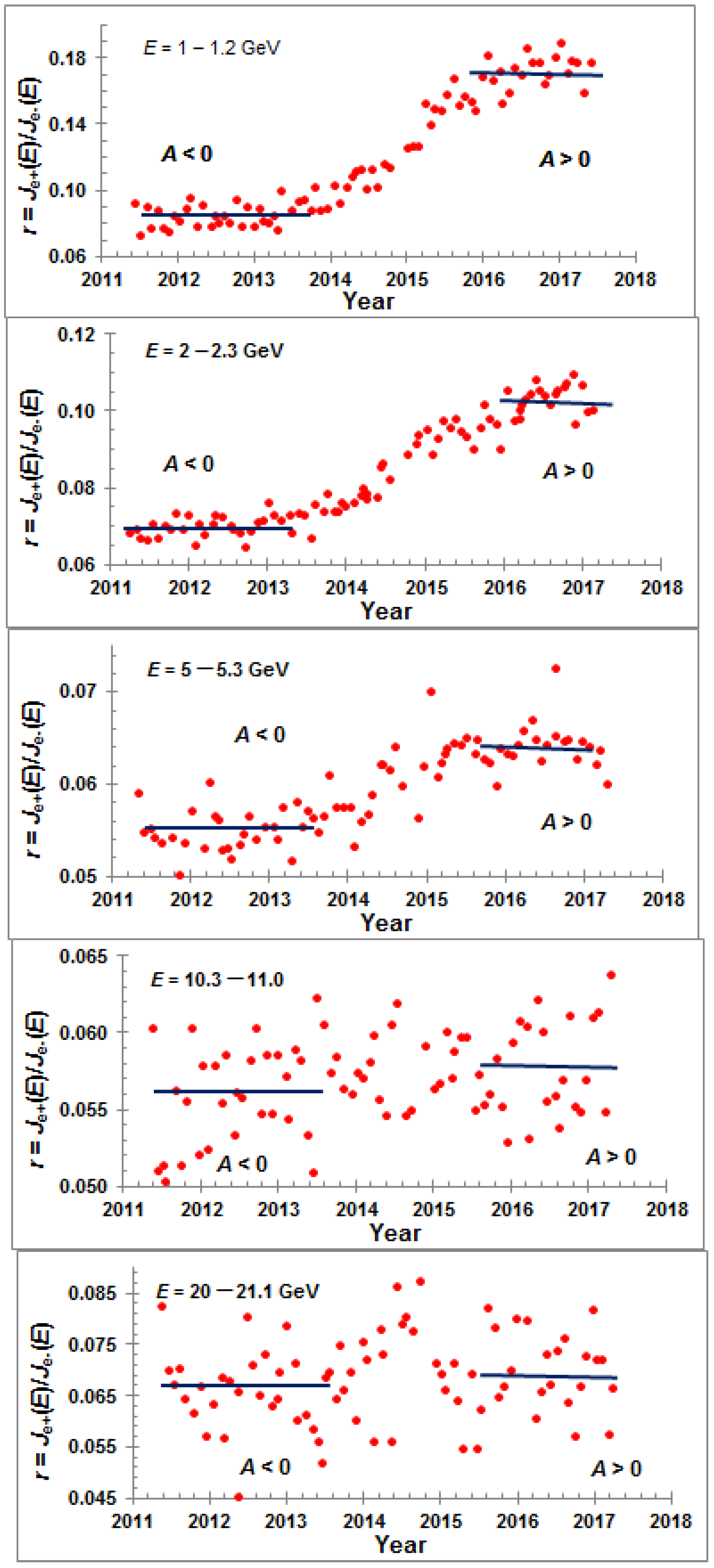
During the transition from the negative phase (A < 0) to the positive one (A > 0), the intensity of positrons (protons and nuclei also) increases; however, electrons (antiprotons) decrease. Let us consider the ratio of positron intensity to electron intensity as a function of the time and energy of these particles,

r (E, t) = J_e+(E, t)/J_e-(E, t)

(3)

where J_e+(E, t) and J_e-(E, t) are the intensities of positrons and electrons, correspondingly [9]. Figure 6 shows the time behavior of this ratio in several energy intervals.

Figure 5 shows the beginning (~2012) and the end (~2015) of the inversion of the polar magnetic field on the Sun, when the transition from the negative phase (A < 0) of the 22-year solar magnetic cycle to the positive one (A > 0) was observed. During the restructuring of magnetic fields in the heliosphere, the intensity of positrons increased, and the intensity of electrons decreased. Thus, the value of r_av has increased.

As one can see from the Figure 6, the difference between the r_av obtained before 2014 and after 2015 decreases with the increase of energy of particles. This ratio r_av becomes close to one at the energy of particles greater than ~10 GeV. This means that in the heliosphere, CR drift effects disappear for high-energy particles. From the data in Figure 6, it follows that an increase of ratio r_av was observed from the middle of 2013 to the middle of 2015 when inversion of the heliospheric magnetic field occurred.

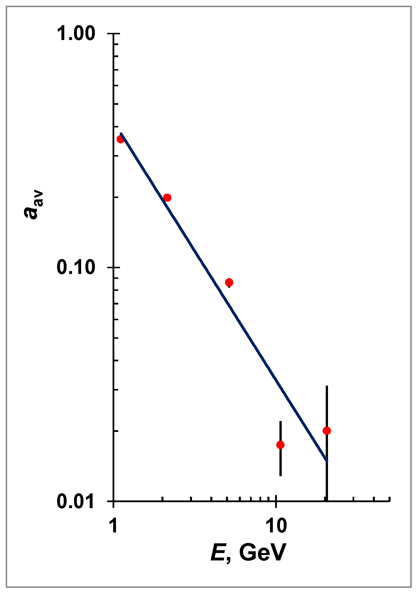
Let us define the amplitude of change of r during the transition from the negative phase to the positive of the 22-year solar magnetic field as

a_av(E) = [r_av(E, A > 0) − r_av(E, A < 0)]/[r_av(E, A > 0) + r_av(E, A < 0)]

(4)

The obtained values of r_av(E, A > 0), r_av(E, A < 0), a_av(E) are given in the

Table 1. The values of the ratio of positron to electron intensities as a function of energy in the positive and negative phases of the 22-year solar magnetic cycle (2011–2017) and the values of a_av(E) (see text).

Energy, GeV	rav(E, A > 0)	rav(E, A < 0)	aav(E)
1.11	0.175 ± 0.008	0.084 ± 0.006	0.353 ± 0.010
2.15	0.104 ± 0.004	0.070± 0.003	0.198 ± 0.005
5.16	0.064 ± 0.003	0.054± 0.003	0.086 ± 0.004
10.68	0.058 ± 0.003	0.054± 0.003	0.017 ± 0.005
20.58	0.069 ± 0.008	0.067 ± 0.008	0.020 ± 0.011

.

As can be seen from the Table 1, the value of a_av(E) decreases with the increase of energy of electrons and positrons. At high energies, the contribution of drifts becomes insignificant in comparison with other mechanisms of modulation (e.g., diffusion process). The dependence of a_av(E) on particle energy is represented on Figure 7, and it scales as a_av(E)= 0.42⋅E⁻¹.

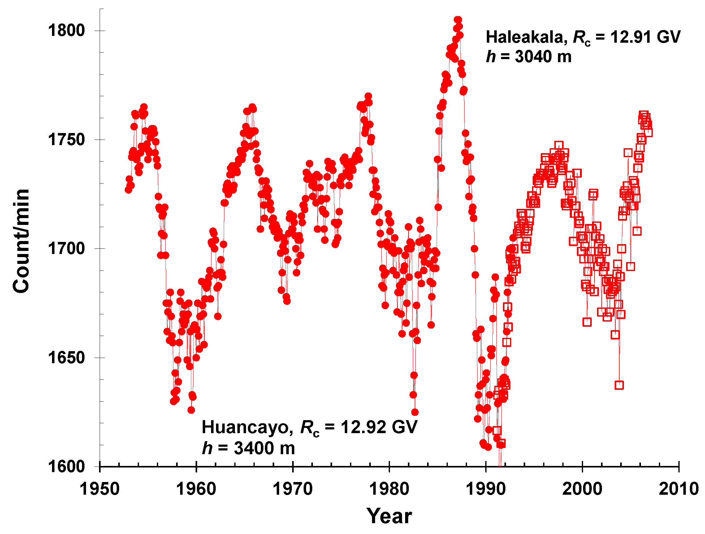
When the value of a_av(E) is near zero (rather small), this means that the drift currents of particles are near zero and also, according to modern ideas, the plateau in time cosmic ray dependence has to be absent. Let us consider high-energy cosmic rays. There are data on cosmic ray fluxes obtained near the equator at a latitude with R_c = 12.9 GV (see Figure 8) [14].

The analysis of data presented in Figure 8 shows that during the negative phases (A < 0) of the 22-year solar magnetic cycle, the time dependence of cosmic rays had peaks (1962–1967 and 1985–1987). During the positive phases (A > 0), plateaus were observed (1973–1978 and 1993–2000). However, the energy of particles falling on the top of the atmosphere at the sites where these neutron monitors were located was more than 12 GeV. As was shown above, the drift currents produced by the particles with such high energies are negligible and cannot be responsible for the formations of peaks or plateaus in the time dependences of CRs (see Table 1 and Figure 7).

5. Discussion

One of the conclusions of modern CR modulation theory is that drifts are responsible for the formation of the plateaus and peaks in the time dependencies of CR fluxes. If one observes a peak for proton flux, electrons will have a plateau, and vice versa. However, the experimental data presented in Figure 4 show that the time dependences of cosmic particles with positive electric charges (protons and nuclei) and negative ones (electrons) have the same form. We have an evident contradiction between the theory and experimental data. Another contradiction comes from the analysis of experimental data of neutron monitors having high geomagnetic cutoff rigidities (R_c = 12.9 GV). In Figure 8, one can see the peaks and plateaus in the experimental data of these devices. These neutron monitors record the secondary particles produced by primaries with energy more than 12 GeV falling on the top of the Earth’s atmosphere. In the time variations of CR fluxes, the drifts of high-energy particles in the heliosphere are very small compared to other CR modulation processes (e.g., the diffusion of CRs). Therefore, the drift effects cannot be responsible for the formation of the peak or plateau in the time profiles of CRs. However, peak- and plateau-like time dependences are observed in the CR data of equatorial neutron monitors. They record secondary particles that are produced by primary cosmic rays with energy E ≥ 12 GeV (see Figure 8).

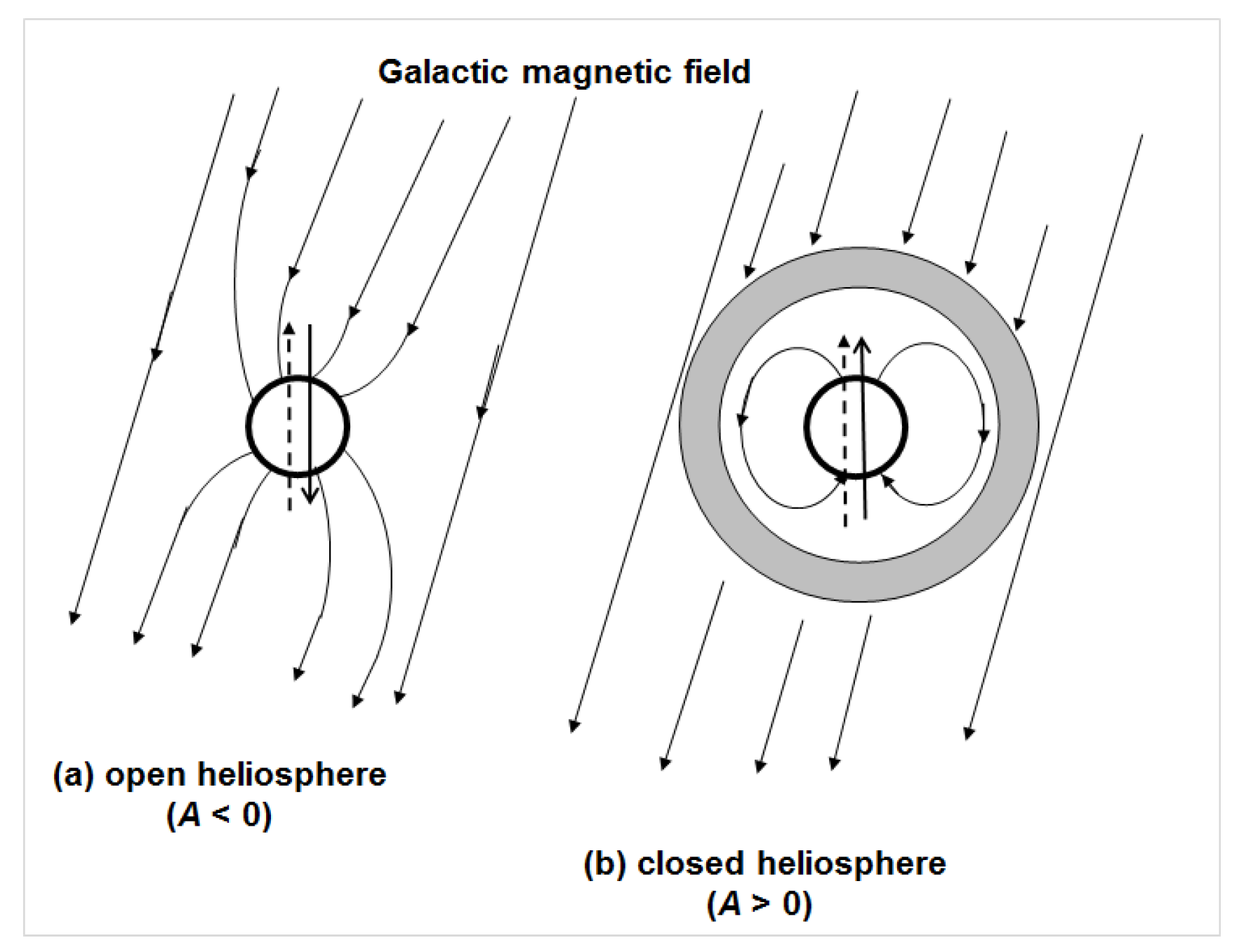
The question arises: what physical mechanism is responsible for the formation of peaks and plateaus in the time dependence of CRs? We suggest that during negative phases of the 22-year solar magnetic cycle, the solar and galactic magnetic field lines are reconnected with each other, and the heliosphere is open for the penetration of cosmic particles from the Galaxy to the solar system. During positive phases, this reconnection is absent and the heliosphere is closed to galactic cosmic ray access. In this case, between the nearby space and the heliosphere, there is a magnetic barrier; the region with a complex and turbulent magnetic field. The thickness of this barrier is from the termination shock (∼85 au.) to the heliopause (∼125 au.) [15,16,17]. The open and closed heliosphere is depicted in Figure 9.

6. Conclusions

The analysis of the experimental data on cosmic rays shows that the appearance of the peaks and plateaus observed in the long-term cosmic ray variations in the heliosphere is not due to drifts of particles in it, as is supposed in modern models of cosmic ray modulation in the heliosphere. The observed peaks and plateau forms are explained by the existence of an open and closed heliosphere for cosmic rays.

In the first case (open heliosphere (A < 0, Ω ↑↑M), there is the reconnection of solar and galactic magnetic field lines, and cosmic rays freely enter the heliosphere. We observe peak-like time dependence in cosmic rays.

In the second case (closed heliosphere (A > 0, Ω ↑↑M), the reconnection of solar and galactic magnetic field lines is absent. Before entering the heliosphere, cosmic rays must overcome the magnetic barrier, which takes up a volume of the termination shock (∼85 au.) to the heliopause (∼125 au.) [17]. We have a plateau-like time dependence in cosmic rays.

It was shown that the drift effects in cosmic rays decrease with the increasing energy of cosmic particles, as ~1/E and are close to zero for particles with E > 10 GeV. However, the data from equatorial neutron monitors, which register secondary particles produced in the Earth’s atmosphere by primary cosmic rays with E > 12 GeV, also show the presence of peaks and plateaus. This indicates that the peak-like and plateau-like time dependences observed in cosmic rays cannot be explained by the particle drift in the heliosphere.