Quintom Fields from Chiral K-Essence Cosmology

Abstract

In this paper, we present an analysis of a chiral cosmological scenario from the perspective of K-essence formalism. In this setup, several scalar fields interact within the kinetic and potential sectors. However, we only consider a flat Friedmann–Robertson–Lamaître–Walker universe coupled minimally to two quintom fields: one quintessence and one phantom. We examine a classical cosmological framework, where analytical solutions are obtained. Indeed, we present an explanation of the “big-bang” singularity by means of a “big-bounce”. Moreover, having a barotropic fluid description and for a particular set of parameters, the phantom line is in fact crossed. Additionally, for the quantum counterpart, the Wheeler–DeWitt equation is analytically solved for various instances, where the factor-ordering problem has been taken into account (measured by the factor Q). Hence, this approach allows us to compute the probability density of the previous two classical subcases. It turns out that its behavior is in effect damped as the scale factor and the scalar fields evolve. It also tends towards the phantom sector when the factor ordering constant $\mathrm{Q}\ll 0$.

1. Introduction

Over the past decades, various cosmological surveys have suggested that two stages of accelerated expansion have occurred during the evolution of the universe [1,2,3,4,5,6]. The first of these epochs, the so-called inflation [5,6], would have happened in a very early stage of the expansion of the cosmos, whilst the second one would be taking place at late times. Additionally, the consensus is that this accelerated expansion is caused by dark energy (DE) [7,8,9]. To account for these phenomena, several cosmological frameworks incorporate scalar fields into their prescriptions and, in fact, they play a preponderant role. Moreover, one of the most studied scenarios in the literature is the quintessence model, which is a fluctuating, homogeneous scalar field that rolls down its scalar potential [10,11,12,13,14,15,16,17]. Different avenues have been explored, broadening the spectrum of scalar field models. For instance, the relevant proposals are the phantom [18,19,20], quintom [21,22,23,24,25,26], and Chiral fields [27,28,29,30,31,32,33,34], and there are many more [35,36,37,38,39,40,41].

However, despite many efforts [7,42,43,44,45,46,47], the nature of dark energy has not yet been deciphered, except for its negative pressure. Accordingly, the main characteristic of DE is given by its equation of state (EoS), defined by the ratio of the pressure-to -energy density, that is, ${\omega }_{DE}\equiv P_{DE}/{\rho }_{DE}$. This definition allows us to classify the cosmological models mentioned above, according to the behavior of the EoS, namely, quintessence $w_Q\ge -1$ [11,48]; phantom $w_P\le -1$ [49,50]; and quintom [51], where the latter is able to evolve across the cosmological constant boundary. In [21], the authors have shown that a single scalar field model does not reproduce the quintom scenario, thus opening a window to new paradigms where additional degrees of freedom can be considered (for non conventional approaches into this matter, we refer the reader to [52,53]).

Our aim is to study a quintom cosmological model. The most basic construction of a quintom model can be achieved by considering a pair of scalar fields, namely, a canonical one and a phantom one, endowed with their respective scalar potentials; within this line of research, different schemes have been considered [21,22,23,24,25,26]. These multi-scalar components bring us additional degrees of freedom; thus, various physical phenomena can be addressed such as primordial, hybrid [54,55,56,57,58], or assisted inflation [59,60], as well as perturbations analysis [61,62].

In this work, we present an analysis of a chiral cosmological scenario from the perspective of K-essence formalism (following the scheme presented in [63]). In this prescription, scalar fields interact within the kinetic and potential sectors. We consider a Friedmann–Robertson–Lamaître–Walker (FRLW) universe coupled minimally to two quintom fields: a quintessence and a phantom. We examine a classical cosmological framework, where exact solutions are obtained. In fact, some of them may indicate that the cosmological singularity is resolved via a “big-bounce”. Moreover, we show that the phantom line is crossed. Lastly, for the quantum counterpart, the Wheeler–DeWitt (WDW) equation is obtained, where the factor-ordering problem takes into account the introduction of the parameter $\mathrm{Q}$, and analytical solutions are presented employing the same relevant cases that appear in the classical scheme. We show that the probability density is in fact damped as the scale factor and the scalar fields evolve.

The paper is laid out as follows. Section 2 is devoted to the analysis of the classical multi-scalar field cosmological model, and analytical solutions are obtained considering different cases. In Section 3, the quantum counterpart is addressed; in this formalism, different cases are analyzed and their corresponding solutions are presented. Section 4 is devoted to the final remarks.

2. Classical Approach

We start by considering the action of the chiral cosmological model from the K-essence perspective, which reads

$$S=\int \sqrt{-g}\left[R-M^{ab}\left({\varphi }_c\right)\mathcal{G}\left({\xi }_{ab}\right)+C\left({\varphi }_c\right)\right]d^{4}x,$$

(1)

where R is the Ricci scalar; $M^{ab}\left({\varphi }_c\right)$ is a matrix related to the kinetic energy mixed terms; $C\left({\varphi }_c\right)$ is the scalar potential, which depends on k scalar fields ($c=1,2,\cdots ,k$); and $\mathcal{G}\left[{\xi }_{ab}\left({\varphi }_c\right)\right]$ is a functional in terms of the chiral kinetic energy ${\xi }_{ab}({\varphi }_c,g^{\mu \nu })=-\frac{1}{2}{g}^{\mu \nu }{\nabla }_{\mu }{\varphi }_a{\nabla }_{\nu }{\varphi }_b$. Note that we are working with the reduced Planck units since $8\pi G=1$, so this eliminates the $8\pi G$ term from the expression (1). An action similar to (1) also appears in modified theories of gravity [64], and more recently in [65]. Making the variation of the action (1) with respect to the fields $(g^{\mu \nu },{\varphi }_c)$, we obtain

$$\begin{array}{cc}\hfill \delta S& =\int \delta \left[\sqrt{-g}R\right]d^{4}x+\int \delta \sqrt{-g}\left[-M^{ab}\left({\varphi }_c\right)\mathcal{G}\left({\xi }_{ab}\right)+C\left({\varphi }_c\right)\right]d^{4}x\hfill \\ \hfill & +\int \sqrt{-g}\left[-\delta M^{ab}\left({\varphi }_c\right)\mathcal{G}\left({\xi }_{ab}\right)-M^{ab}\left({\varphi }_c\right)\delta \mathcal{G}\left({\xi }_{ab}\right)+\delta C\left({\varphi }_c\right)\right]d^{4}x,\hfill \\ \hfill & =\int \sqrt{-g}{G}_{\lambda \theta }\delta g^{\lambda \theta }{d}^{4}x-\int \sqrt{-g}\frac{1}{2}\left[-M^{ab}\left(\varphi \right)\mathcal{G}\left({\xi }_{ab}\right)+C\left({\varphi }_c\right)\right]g_{\lambda \theta }\delta g^{\lambda \theta }{d}^{4}x+\hfill \\ \hfill & +\int \sqrt{-g}\left[-\frac{\partial M^{ab}\left({\varphi }_c\right)}{\partial {\varphi }_c}\delta {\varphi }_c\mathcal{G}\left({\xi }_{ab}\right)-M^{ab}\left({\varphi }_c\right)\frac{\partial \mathcal{G}\left({\xi }_{ab}\right)}{\partial {\xi }_{ab}}\delta {\xi }_{ab}+\frac{\partial C\left({\varphi }_c\right)}{\partial \varphi }\delta {\varphi }_c\right]d^{4}x,\hfill \end{array}$$

(2)

where $G_{\lambda \theta }=R_{\lambda \theta }-R{g}_{\lambda \theta }/2$, $R_{\lambda \theta }$, and $g_{\lambda \theta }$ are the Einstein, Ricci, and metric tensors, respectively. The variation of the functional $\mathcal{G}\left({\xi }_{ab}\right)$ is

$$\begin{array}{cc}\hfill \delta {\xi }_{ab}\left({\varphi }_c\right)& =-\frac{1}{2}{\nabla }_{\mu }{\varphi }_a{\nabla }_{\nu }{\varphi }_b\delta g^{\mu \nu }-\frac{1}{2}{g}^{\mu \nu }{\nabla }_{\mu }\delta {\varphi }_a{\nabla }_{\nu }{\varphi }_b-\frac{1}{2}{g}^{\mu \nu }{\nabla }_{\mu }{\varphi }_a{\nabla }_{\nu }\delta {\varphi }_b,\hfill \\ \hfill & =-\frac{1}{2}{\nabla }_{\mu }{\varphi }_a{\nabla }_{\nu }{\varphi }_b\delta g^{\mu \nu }+\frac{1}{2}{\nabla }_{\mu }\left[g^{\mu \nu }{\nabla }_{\nu }{\varphi }_b\right]\delta {\varphi }_a+\frac{1}{2}{\nabla }_{\nu }\left[g^{\mu \nu }{\nabla }_{\mu }{\varphi }_a\right]\delta {\varphi }_b\hfill \\ \hfill & +{\nabla }_{\mu }\left[\frac{1}{2}\delta {\varphi }_a{g}^{\mu \nu }{\nabla }_{\nu }{\varphi }_b\right]+{\nabla }_{\nu }\left[\frac{1}{2}\delta {\varphi }_b{g}^{\mu \nu }{\nabla }_{\nu }{\varphi }_a\right].\hfill \end{array}$$

Thus, finally we have

$$\begin{array}{cc}\hfill \delta S& =\int \sqrt{-g}\left\{G_{\mu \nu }+\frac{1}{2}{M}^{ab}\left({\varphi }_c\right)\left[{\nabla }_{\mu }{\varphi }_a{\nabla }_{\nu }{\varphi }_b\frac{\partial \mathcal{G}\left({\xi }_{ab}\right)}{\partial {\xi }_{ab}}+g_{\mu \nu }\mathcal{G}\left({\xi }_{ab}\right)\right]\right.\hfill \\ \hfill & \left.-\frac{1}{2}{g}_{\mu \nu }C\left({\varphi }_c\right)\right\}\delta g^{\mu \nu }{d}^{4}x,\hfill \end{array}$$

and since $\delta \mathcal{S}$ vanishes ($\delta \mathcal{S}=0$) for arbitrary variations $\delta g^{\mu \nu }$, we are led to the field equations

$$G_{\mu \nu }=-\frac{1}{2}{M}^{ab}\left({\varphi }_c\right)\left[{\nabla }_{\mu }{\varphi }_a{\nabla }_{\nu }{\varphi }_b\frac{\partial \mathcal{G}\left({\xi }_{ab}\right)}{\partial {\xi }_{ab}}+g_{\mu \nu }\mathcal{G}\left({\xi }_{ab}\right)\right]+\frac{1}{2}{g}_{\mu \nu }C\left({\varphi }_c\right).$$

(3)

Then, the energy-momentum tensor in this setup becomes

$$T_{\mu \nu }\left({\varphi }_c\right)=+\frac{1}{2}{M}^{ab}\left({\varphi }_c\right)\left[{\nabla }_{\mu }{\varphi }_a{\nabla }_{\nu }{\varphi }_b\frac{\partial \mathcal{G}\left({\xi }_{ab}\right)}{\partial {\xi }_{ab}}+g_{\mu \nu }\mathcal{G}\left({\xi }_{ab}\right)\right]-\frac{1}{2}{g}_{\mu \nu }C\left({\varphi }_c\right).$$

(4)

Moreover, we consider the energy-momentum tensor of a barotropic perfect fluid $T_{\alpha \beta }\left({\varphi }_c\right)=(\rho +P)u_{\alpha }\left({\varphi }_c\right)u_{\beta }\left({\varphi }_c\right)+P{g}_{\alpha \beta }$ (where the four-velocity is given by $u_{\alpha }{u}_{\beta }={\nabla }_{\alpha }{\varphi }_a{\nabla }_{\beta }{\varphi }_b/2{\xi }_{ab}$). Hence, the pressure P and the energy density $\rho$ of the scalar fields take the following form:

$$P\left({\varphi }_c\right)=\frac{1}{2}{M}^{ab}\left({\varphi }_c\right)\mathcal{G}-\frac{1}{2}C\left({\varphi }_c\right),\rho \left({\varphi }_c\right)=\frac{1}{2}{M}^{ab}\left[2{\xi }_{ab}\frac{\partial \mathcal{G}}{\partial {\xi }_{ab}}-\mathcal{G}\right]+\frac{1}{2}C\left({\varphi }_c\right).$$

(5)

Additionally, the barotropic parameter ${\omega }_{{\xi }_{ab}}$ becomes

$${\omega }_{{\xi }_{ab}}=\frac{P\left({\varphi }_c\right)}{\rho \left({\varphi }_c\right)}=\frac{M^{ab}\left({\varphi }_c\right)\mathcal{G}-C\left({\varphi }_c\right)}{M^{ab}\left[2{\xi }_{ab}\frac{\partial \mathcal{G}}{\partial {\xi }_{ab}}-\mathcal{G}\right]+C\left({\varphi }_c\right)}.$$

(6)

On the other hand, taking the variation of the action (1) with respect to the scalar field ${\varphi }_c$, we obtain

$$\begin{array}{ccc}& & \delta S=\int \sqrt{g}\left\{-\frac{\partial M^{ab}\left({\varphi }_c\right)}{\partial {\varphi }_c}\mathcal{G}\left({\xi }_{ab}\right)-\frac{1}{2}{M}^{cb}\left({\varphi }_c\right)\frac{\partial \mathcal{G}\left({\xi }_{ab}\right)}{\partial {\xi }_{ab}}{\nabla }_{\nu }{\nabla }^{\nu }{\varphi }_b\right.\hfill \\ & & \left.-\frac{1}{2}{M}^{ac}\left({\varphi }_c\right)\frac{\partial \mathcal{G}\left({\xi }_{ab}\right)}{\partial {\xi }_{ab}}{\nabla }_{\nu }{\nabla }^{\nu }{\varphi }_a+\frac{\partial C\left({\varphi }_c\right)}{\partial {\varphi }_c}\right\}\delta {\varphi }_c{d}^{4}x,\hfill \end{array}$$

where a Klein-Gordon-like equation can be written as follows:

$$\frac{\partial M^{ab}\left({\varphi }_c\right)}{\partial {\varphi }_c}\mathcal{G}\left({\xi }_{ab}\right)-M^{ac}\left({\varphi }_c\right)\frac{\partial \mathcal{G}\left({\xi }_{ab}\right)}{\partial {\xi }_{ab}}{\nabla }_{\nu }{\nabla }^{\nu }{\varphi }_a-\frac{\partial C\left({\varphi }_c\right)}{\partial {\varphi }_c}=0.$$

(7)

Note that Equations (2)–(7) represent the general framework; however, we will particularize to the case $\mathcal{G}=\xi$, therefore obtaining the standard chiral Einstein field equations

$$G_{\mu \nu }=-\frac{1}{2}{M}^{ab}\left({\varphi }_c\right)\left[{\nabla }_{\mu }{\varphi }_a{\nabla }_{\nu }{\varphi }_b-\frac{1}{2}{g}_{\mu \nu }{g}^{\alpha \beta }{\nabla }_{\alpha }{\varphi }_a{\nabla }_{\beta }{\varphi }_b\right]+\frac{1}{2}{g}_{\mu \nu }C\left({\varphi }_c\right).$$

(8)

Now, if we consider that $M^{ab}$ is a constant matrix, we obtain

$$M^{ac}{\nabla }_{\nu }{\nabla }^{\nu }{\varphi }_a-\frac{\partial C\left({\varphi }_c\right)}{\partial {\varphi }_c}=0.$$

(9)

All of the aforementioned results can be employed to consider a two-field cosmological model: a quintessence and a phantom field, with their corresponding scalar potentials. Setting $M^{ab}\left({\varphi }_c\right)=m^{ab}$ as a constant matrix, in (1), we obtain

$$\mathcal{L}=\sqrt{-g}\left(R-\frac{1}{2}{g}^{\mu \nu }{m}^{ab}{\nabla }_{\mu }{\varphi }_a{\nabla }_{\nu }{\varphi }_b+V({\varphi }_1,{\varphi }_2)\right),$$

(10)

where $C\left({\varphi }_c\right)=V({\varphi }_1,{\varphi }_2)$ is the combined scalar field potential; ${\varphi }_1$ and ${\varphi }_2$ are the quintessence and phantom fields, respectively; and $m^{ab}$ is a $2\times 2$ constant matrix of the form $m^{ab}=\left(\begin{array}{cc}1& m^{12}\\ \hfill m^{12}& -1\end{array}\right).$

Thus, the Einstein–Klein–Gordon field Equations (8) and (9) are

$$G_{\alpha \beta }=-\frac{1}{2}{m}^{ab}\left({\nabla }_{\alpha }{\varphi }_a{\nabla }_{\beta }{\varphi }_b-\frac{1}{2}{g}_{\alpha \beta }{g}^{\mu \nu }{\nabla }_{\mu }{\varphi }_a{\nabla }_{\nu }{\varphi }_b\right)+\frac{1}{2}{g}_{\alpha \beta }V({\varphi }_1,{\varphi }_2),$$

(11)

$$m^{cb}{\nabla }_{\nu }{\nabla }^{\nu }{\varphi }_b-\frac{\partial C\left({\varphi }_c\right)}{\partial {\varphi }_c}=0,$$

(12)

where $a,b,c=1,2$. From (11), the energy-momentum tensor of the scalar fields $({\varphi }_1,{\varphi }_2)$ is given by

$$8\pi G{T}_{\alpha \beta }({\varphi }_1,{\varphi }_2)=-\frac{1}{2}{m}^{ab}\left({\nabla }_{\alpha }{\varphi }_a{\nabla }_{\beta }{\varphi }_b-\frac{1}{2}{g}_{\alpha \beta }{g}^{\mu \nu }{\nabla }_{\mu }{\varphi }_a{\nabla }_{\nu }{\varphi }_b\right)+\frac{1}{2}{g}_{\alpha \beta }V({\varphi }_1,{\varphi }_2),$$

(13)

then, using (6), the barotropic index ${\omega }_{{\varphi }_a,{\varphi }_b}$ is given by

$${\omega }_{{\varphi }_a{\varphi }_b}=\frac{-\frac{1}{2}{m}^{ab}{\nabla }^{\mu }{\varphi }_a{\nabla }_{\mu }{\varphi }_b-C\left({\varphi }_c\right)}{-\frac{1}{2}{m}^{ab}{\nabla }^{\mu }{\varphi }_a{\nabla }_{\mu }{\varphi }_b+C\left({\varphi }_c\right)}.$$

(14)

In our analysis, the background spacetime to be considered is a spatially flat FRLW with line element

$$d{s}^2=-N{\left(t\right)}^{2}d{t}^2+e^{2\Omega \left(t\right)}\left[d{r}^2+r^2(d{\theta }^2+si{n}^2\theta d{\varphi }^2)\right],$$

(15)

where N represents the lapse function, $A\left(t\right)=e^{\Omega \left(t\right)}$ is the scale factor in the Misner parametrization, and $\Omega$ is a scalar function whose interval is $(-\infty ,\infty )$. Choosing $C\left({\varphi }_c\right)=V_1\left({\varphi }_1\right)+V_2\left({\varphi }_2\right)=V_{01}{e}^{-{\lambda }_1{\varphi }_1}+V_{02}{e}^{-{\lambda }_2{\varphi }_2}$, the mixed Einstein field equations are

$$\begin{array}{cc}\hfill 3\frac{{\dot{\Omega }}^2}{N^2}-\frac{1}{2}\left[\frac{1}{2}\frac{{\dot{\varphi }}_1^2}{N^2}+V_1\left({\varphi }_1\right)\right]-\frac{1}{2}\left[-\frac{1}{2}\frac{{\dot{\varphi }}_2^2}{N^2}+V_2\left({\varphi }_2\right)\right]-\frac{m^{12}}{2}\frac{{\dot{\varphi }}_1}{N}\frac{{\dot{\varphi }}_2}{N}& =0,\hfill \end{array}$$

(16)

$$\begin{array}{cc}\hfill 2\frac{\ddot{\Omega }}{N^2}+3\frac{{\dot{\Omega }}^2}{N^2}-2\frac{\dot{\Omega }}{N}\frac{\dot{N}}{N^2}+\frac{1}{2}\left[\frac{1}{2}\frac{{\dot{\varphi }}_1^2}{N^2}-V_1\left({\varphi }_1\right)\right]+\frac{1}{2}\left[-\frac{1}{2}\frac{{\dot{\varphi }}_2^2}{N^2}-V_2\left({\varphi }_2\right)\right]+\frac{m^{12}}{2}\frac{{\dot{\varphi }}_1}{N}\frac{{\dot{\varphi }}_2}{N}& =0,\hfill \end{array}$$

(17)

$$\begin{array}{cc}\hfill {\dot{\varphi }}_1\left(-3\frac{\dot{\Omega }}{N}\frac{{\dot{\varphi }}_1}{N}+\frac{\dot{N}}{N^2}\frac{{\varphi }_1}{N}-\frac{{\ddot{\varphi }}_1}{N^2}\right)+m^{12}{\dot{\varphi }}_1\left(-3\frac{\dot{\Omega }}{N}\frac{{\dot{\varphi }}_2}{N}+\frac{\dot{N}}{N^2}\frac{{\varphi }_2}{N}-\frac{{\ddot{\varphi }}_2}{N^2}\right)-{\dot{V}}_1\left({\varphi }_1\right)& =0,\hfill \end{array}$$

(18)

$$\begin{array}{cc}\hfill m^{12}{\dot{\varphi }}_2\left(-3\frac{\dot{\Omega }}{N}\frac{{\dot{\varphi }}_1}{N}+\frac{\dot{N}}{N^2}\frac{{\varphi }_1}{N}-\frac{{\ddot{\varphi }}_1}{N^2}\right)+{\dot{\varphi }}_2\left(3\frac{\dot{\Omega }}{N}\frac{{\dot{\varphi }}_2}{N}-\frac{\dot{N}}{N^2}\frac{{\varphi }_2}{N}+\frac{{\ddot{\varphi }}_2}{N^2}\right)-{\dot{V}}_2\left({\varphi }_2\right)& =0,\hfill \end{array}$$

(19)

where “$·$” represents a time derivative. By plugging the line element (15) into the energy-momentum tensor of the scalar fields (13), the energy density, and the pressure, the following form is taken:

$$\begin{array}{cc}\hfill 8\pi G{\rho }_{{\varphi }_1{\varphi }_2}& =\frac{1}{2}\left[\frac{1}{2}{\dot{\varphi }}_1^2+N^2{V}_1\left({\varphi }_1\right)\right]+\frac{1}{2}\left[-\frac{1}{2}{\dot{\varphi }}_2^2+N^2{V}_2\left({\varphi }_2\right)\right]+\frac{m^{12}}{2}{\dot{\varphi }}_1{\dot{\varphi }}_2,\hfill \end{array}$$

(20)

$$\begin{array}{cc}\hfill 8\pi G{P}_{{\varphi }_1{\varphi }_2}& =\frac{1}{2}\left[\frac{1}{2}\frac{{\dot{\varphi }}_1^2}{N^2}-V_1\left({\varphi }_1\right)\right]+\frac{1}{2}\left[-\frac{1}{2}\frac{{\dot{\varphi }}_2^2}{N^2}-V_2\left({\varphi }_2\right)\right]+\frac{m^{12}}{2}\frac{{\dot{\varphi }}_1}{N}\frac{{\dot{\varphi }}_2}{N},\hfill \end{array}$$

(21)

having these two quantities at hand, the barotropic parameter will be written as

$${\omega }_{{\varphi }_1{\varphi }_2}=\frac{P_{{\varphi }_1{\varphi }_2}}{{\rho }_{{\varphi }_1{\varphi }_2}}=\frac{\left[\frac{1}{2}\frac{{\dot{\varphi }}_1^2}{N^2}-V_1\left({\varphi }_1\right)\right]+\left[-\frac{1}{2}\frac{{\dot{\varphi }}_2^2}{N^2}-V_2\left({\varphi }_2\right)\right]+m^{12}\frac{{\dot{\varphi }}_1}{N}\frac{{\dot{\varphi }}_2}{N}}{\left[\frac{1}{2}{\dot{\varphi }}_1^2+N^2{V}_1\left({\varphi }_1\right)\right]+\left[-\frac{1}{2}{\dot{\varphi }}_2^2+N^2{V}_2\left({\varphi }_2\right)\right]+m^{12}{\dot{\varphi }}_1{\dot{\varphi }}_2}.$$

(22)

Now we are in position to construct the corresponding Lagrangian and Hamiltonian densities for this cosmological model. Using Hamilton’s approach, classical solutions to EKG (16)–(19) can be found; additionally, the quantum counterpart can be established and solved. Taking these ideas into consideration, putting back the metric (15) into (10), the Lagrangian density reads

$$\mathcal{L}=e^{3\Omega }\left(\frac{6{\dot{\Omega }}^2}{N}-\frac{{\dot{{\varphi }_1}}^2}{2N}+\frac{{\dot{{\varphi }_2}}^2}{2N}-\frac{m^{12}\dot{{\varphi }_1}{\dot{\varphi }}_2}{N}+N{V}_{01}{e}^{-{\lambda }_1{\varphi }_1}+N{V}_{02}{e}^{-{\lambda }_2{\varphi }_2}\right).$$

(23)

The resulting momenta are given by

$$\begin{array}{cc}\hfill {\Pi }_{\Omega }& =12\frac{e^{3\Omega }}{N}\dot{\Omega },\hfill \\ \hfill {\Pi }_{{\varphi }_1}& =-\frac{e^{3\Omega }}{N}\left({\dot{\varphi }}_1+m^{12}{\dot{\varphi }}_2\right),\hfill \\ \hfill {\Pi }_{{\varphi }_2}& =-\frac{e^{3\Omega }}{N}\left(m^{12}{\dot{\varphi }}_1-{\dot{\varphi }}_2\right),\hfill \end{array}\begin{array}{cc}\hfill \dot{\Omega }& =\frac{N{e}^{-3\Omega }}{12}{\Pi }_{\Omega },\hfill \\ \hfill {\dot{\varphi }}_1& =-\frac{N{e}^{-3\Omega }}{▵}\left({\Pi }_{{\varphi }_1}+m^{12}{\Pi }_{{\varphi }_2}\right),\hfill \\ \hfill {\varphi }_2& =\frac{N{e}^{-3\Omega }}{▵}\left(m^{12}{\Pi }_{{\varphi }_1}-{\Pi }_{{\varphi }_2}\right),\hfill \end{array}$$

(24)

where $▵=1+{\left(m^{12}\right)}^2$. In order to obtain a Hamiltonian density, we write (23) in a canonical form, i.e., ${\mathcal{L}}_{can}={\Pi }_q\dot{q}-N\mathcal{H}$; then, we perform the variation with respect to the lapse function N, $\delta {\mathcal{L}}_{can}/\delta N=0$, yielding the Hamiltonian constraint $\mathcal{H}=0$, that is,

$$\mathcal{H}=\frac{e^{-3\Omega }}{24}\left[{\Pi }_{\Omega }^2-\frac{12}{▵}{\Pi }_{{\varphi }_1}^2+\frac{12}{▵}{\Pi }_{{\varphi }_2}^2-24\frac{m^{12}}{▵}{\Pi }_{{\varphi }_1}{\Pi }_{{\varphi }_2}-24V_1{e}^{-{\lambda }_1{\varphi }_1+6\Omega }-24V_2{e}^{-{\lambda }_2{\varphi }_2+6\Omega }\right].$$

(25)

The fact that $\mathcal{H}=0$ guarantees us that its solutions are unique and well defined. Putting forward the following canonical transformation on the variables $(\Omega ,{\varphi }_1,{\varphi }_2)\leftrightarrow ({\xi }_1,{\xi }_2,{\xi }_3)$ and fixing the gauge $N=24e^{3\Omega }$, we obtain

$$\begin{array}{cc}\hfill {\xi }_1& =6\Omega -{\lambda }_1{\varphi }_1,\hfill \\ \hfill {\xi }_2& =6\Omega -{\lambda }_2{\varphi }_2,\hfill \\ \hfill {\xi }_3& =6\Omega +{\lambda }_1{\varphi }_1+{\lambda }_2{\varphi }_2,\hfill \end{array}⟷\begin{array}{cc}\hfill \Omega & =\frac{{\xi }_1+{\xi }_2+{\xi }_3}{18},\hfill \\ \hfill {\varphi }_1& =\frac{-2{\xi }_1+{\xi }_2+{\xi }_3}{3{\lambda }_1},\hfill \\ \hfill {\varphi }_2& =\frac{{\xi }_1-2{\xi }_2+{\xi }_3}{3{\lambda }_2},\hfill \end{array}$$

(26)

leading us to obtain a new set of conjugate momenta $(P_1,P_2,P_3)$

$$\begin{array}{cc}\hfill {\Pi }_{\Omega }& =6P_1+6P_2+6P_3,\hfill \\ \hfill {\Pi }_{{\varphi }_1}& ={\lambda }_1\left(-P_1+P_3\right),\hfill \\ \hfill {\Pi }_{{\varphi }_2}& ={\lambda }_2\left(-P_2+P_3\right),\hfill \end{array}$$

(27)

therefore, the Hamiltonian density can be written as

$$\begin{array}{cc}\hfill \mathcal{H}& =12\left(3-{\Lambda }_1\right)P_1^2+12\left(3+{\Lambda }_2\right)P_2^2+12\left(3-2{\Lambda }_{12}+{\Lambda }_2-{\Lambda }_1\right)P_3^2\hfill \\ \hfill & +24\left[\left(3+{\Lambda }_1+{\Lambda }_{12}\right)P_1+\left(3+{\Lambda }_{12}-{\Lambda }_2\right)P_2\right]P_3\hfill \\ \hfill & +24\left(3-{\Lambda }_{12}\right)P_1{P}_2-24\left(V_1{e}^{{\xi }_1}+V_2{e}^{{\xi }_2}\right),\hfill \end{array}$$

(28)

where ${\Lambda }_1={\lambda }_1^2/▵$, ${\Lambda }_2={\lambda }_2^2/▵$, and ${\Lambda }_{12}=m^{12}{\lambda }_1{\lambda }_2/▵$. In the end, even if the Hamiltonian density (28) exhibits an intricate form, this configuration will indeed allow us to compute various relevant scenarios. Thus, the Hamilton equations become

$$\begin{array}{cc}\hfill {\dot{\xi }}_1& =24\left(3-{\Lambda }_1\right)P_1+24\left(3-{\Lambda }_{12}\right)P_2+24\left(3+{\Lambda }_1+{\Lambda }_{12}\right)P_3,\hfill \\ \hfill {\dot{\xi }}_2& =24\left(3+{\Lambda }_2\right)P_2+24\left(3-{\Lambda }_{12}\right)P_1+24\left(3-{\Lambda }_2+{\Lambda }_{12}\right)P_3,\hfill \\ \hfill {\dot{\xi }}_3& =24\left(3+{\Lambda }_1+{\Lambda }_{12}\right)P_1+24\left(3-{\Lambda }_2+{\Lambda }_{12}\right)P_2+24\left(3+{\Lambda }_2-{\Lambda }_1-2{\Lambda }_{12}\right)P_3,\hfill \\ \hfill {\dot{P}}_1& =24V_1{e}^{{\xi }_1},\hfill \\ \hfill {\dot{P}}_2& =24V_2{e}^{{\xi }_2},\hfill \\ \hfill {\dot{P}}_3& =0.\hfill \end{array}$$

(29)

Right away, we can see that $P_3=p_3=constant$. Moreover, the end game of this analysis is to find solutions to the variables ($\Omega ,{\varphi }_1,{\varphi }_2$). Hence, we simplify our expression. First, we drop the mixed momenta $P_1$ and $P_2$ from ${\dot{\xi }}_1$ and ${\dot{\xi }}_2$ (Equation (29)) by setting their coefficients to zero: $3-{\Lambda }_{12}=0$. Therefore, we can obtain one relation among the parameters $(m^{12},{\lambda }_1{\lambda }_2)$, where the matrix element $m^{12}$ satisfies the constraint

$$m^{12}=\frac{{\lambda }_1{\lambda }_2}{6}\left[1\pm \sqrt{1-{\left(\frac{6}{{\lambda }_1{\lambda }_2}\right)}^2}\right].$$

(30)

Additionally, we set the second term inside the square root of (30) to be a real number and consider ${\lambda }_1>0$, ${\lambda }_2>0$, thus yielding the relation ${\lambda }_1{\lambda }_2\ge 6$, ensuring that $m^{12}$ is always positive.

2.1. Classical Exact Solutions

In this section, we will calculate the exact solutions of ($\Omega ,{\varphi }_1,{\varphi }_2$), where different cases will appear due to the parameters $({\lambda }_1,{\lambda }_2)$. Recall the master Hamiltonian density

$$\begin{array}{cc}\hfill \mathcal{H}& =12{\eta }_1{P}_1^2+12{\eta }_2{P}_2^2+12\left(-9+{\eta }_1+{\eta }_2\right)p_3^2+24\left[\left(9-{\eta }_1\right)P_1+\left(9-{\eta }_2\right)P_2\right]p_3\hfill \\ \hfill & -24\left(V_1{e}^{{\xi }_1}+V_2{e}^{{\xi }_2}\right),\hfill \end{array}$$

(31)

with ${\eta }_1=3-{\Lambda }_1$ and ${\eta }_2=3+{\Lambda }_2$. Then, Hamilton equations for these new coordinates ${\xi }_i$ are

$$\begin{array}{ccc}\hfill {\dot{\xi }}_1& =& 24{\eta }_1{P}_1+24\left(9-{\eta }_1\right)p_3,\hfill \\ \hfill {\dot{\xi }}_2& =& 24{\eta }_2{P}_2+24\left(9-{\eta }_2\right)p_3,\hfill \\ \hfill {\dot{\xi }}_3& =& 24\left(9-{\eta }_1\right)P_1+24\left(9-{\eta }_2\right)P_2+24\left(-9+{\eta }_1+{\eta }_2\right)p_3,\hfill \end{array}$$

(32)

and equations for ${\dot{P}}_1$ and ${\dot{P}}_2$ are still given by (29). In the following sections, we will obtain analytical solutions for differents values of ${\lambda }_1$ and ${\lambda }_2$.

2.1.1. Case: ${\lambda }_1={\lambda }_2=\sqrt{6}$

For these particular values, we have ${\Lambda }_1={\Lambda }_2=3$ with ${\eta }_1=0$ and ${\eta }_2=6$; then, the Hamilton equations are reduced to

$$\begin{array}{ccc}\hfill {\dot{\xi }}_1& =& 216p_3,\hfill \\ \hfill {\dot{\xi }}_2& =& 144P_2+72p_3,\hfill \\ \hfill {\dot{\xi }}_3& =& 216P_1+72P_2-72p_3.\hfill \end{array}$$

(33)

From the last set of equations, we can see that the solution for ${\dot{\xi }}_1$ will be given by

$${\xi }_1=a_1+216p_{3}t,$$

(34)

where $a_1$ is an integration constant. Then, taking the time derivative of ${\dot{\xi }}_2$ results in ${\ddot{\xi }}_2=3456V_2{e}^{{\xi }_2}$, whose solution is

$${\xi }_2=Ln\left(\frac{{\alpha }_2^2}{1728V_2}\right)+Ln\left[Csc{h}^2({\alpha }_{2}t-{\beta }_2)\right].$$

(35)

Now we know the functional form of ${\xi }_2$, we can compute the remaining momenta, yielding

$$\begin{array}{ccc}\hfill P_1\left(t\right)& =& p_1+\frac{V_1}{9p_3}{e}^{a_1+216p_{3}t},\hfill \\ \hfill P_2\left(t\right)& =& p_2-\frac{{\alpha }_2}{72}Coth({\alpha }_{2}t-{\beta }_2).\hfill \end{array}$$

(36)

Plugging back $P_1$ and $P_2$, given by (36), into the Hamiltonian constraint $\mathcal{H}=0$, we found that $p_2=-p_3/2$ and $3888p_3^2-\mathrm{15,552}{p}_1{p}_3-{\alpha }_2^2=0$; solving for $p_3$ gives $p_3=2p_1\pm \frac{\sqrt{3}}{108}\sqrt{{\alpha }_2^2+\mathrm{15,552}{p}_1^2}$.

With these results, the variable ${\xi }_3$ becomes

$${\xi }_3=a_3+(216p_1-108p_3)t+\frac{V_1}{9p_3^2}{e}^{a_1+216p_{3}t}+Ln\left[Csch\left({\alpha }_{2}t-{\beta }_2\right)\right].$$

(37)

where $a_3$ is an integration constant. Having found ${\xi }_1$, ${\xi }_2$, and ${\xi }_3$ and then applying the inverse transformation (26), we can present the solutions in the original variables

$$\begin{array}{cc}\hfill \Omega \left(t\right)& =\frac{a_1+a_3}{18}+Ln{\left[\frac{{\alpha }_2}{24\sqrt{3V_2}}\right]}^{\frac{1}{9}}\hfill \\ \hfill & +Ln\left[Csc{h}^{\frac{1}{6}}\left({\alpha }_{2}t-{\beta }_2\right)\right]+(12p_1+6p_3)t+\frac{V_1}{162p_3^2}{e}^{a_1+216p_{3}t},\hfill \end{array}$$

(38)

$$\begin{array}{cc}\hfill {\varphi }_1\left(t\right)& =\frac{-2a_1+a_3}{3{\lambda }_1}+Ln{\left(\frac{{\alpha }_2^2}{1728V_2}\right)}^{\frac{1}{3{\lambda }_1}}\hfill \\ \hfill & +\frac{1}{{\lambda }_1}\left[\left(72p_1-180p_3\right)t+\frac{V_1}{27p_3^2}{e}^{a_1+216p_{3}t}+Ln\left[Csch\left({\alpha }_{2}t-{\beta }_2\right)\right]\right],\hfill \end{array}$$

(39)

$$\begin{array}{cc}\hfill {\varphi }_2\left(t\right)& =\frac{a_1+a_3}{3{\lambda }_2}+Ln{\left(\frac{{\alpha }_2^2}{1728V_2}\right)}^{-\frac{2}{3{\lambda }_2}}\hfill \\ \hfill & +\frac{1}{{\lambda }_2}\left[\left(72p_1+36p_3\right)t+\frac{V_1}{27p_3^2}{e}^{a_1+216p_{3}t}+Ln\left[Sinh\left({\alpha }_{2}t-{\beta }_2\right)\right]\right],\hfill \end{array}$$

(40)

Recalling that the scale factor is given by $A\left(t\right)=e^{\Omega \left(t\right)}$, we have

$$A\left(t\right)=e^{\frac{a_1+a_3}{18}}{\left[\frac{{\alpha }_2}{24\sqrt{3V_2}}\right]}^{\frac{1}{9}}Csc{h}^{\frac{1}{6}}\left({\alpha }_{2}t-{\beta }_2\right)Exp\left[\frac{V_1}{162p_3^2}{e}^{a_1+216p_{3}t}\right]e^{(12p_1+6p_3)t}.$$

(41)

In Figure 1, we present the behaviour of the scale factor $A=A\left(t\right)$, the Hubble parameter $H=H\left(t\right)$, and the barotropic parameter ${\omega }_{{\varphi }_1{\varphi }_2}={\omega }_{{\varphi }_1{\varphi }_2}\left(t\right)$. From the upper left graph, we can see that A grows very rapidly as time goes by; it can also be seen that this solution avoids the singularity by means of a bounce, where H does cross the horizontal axis. In the panel at the bottom, the barotropic parameter ${\omega }_{{\varphi }_1{\varphi }_2}$ is presented, and it can be seen that the EoS parameter crosses the “−1” boundary, which is in fact a characteristic of the quintom models.

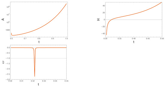
Figure 1. This figure shows the time ($0.3\le t\le 1.0$) evolution of the scale factor $A\left(t\right)$, the Hubble parameter $H\left(t\right)$, and the barotropic parameter ${\omega }_{{\varphi }_1{\varphi }_2}\left(t\right)$. We use arbitrary units, namely, $V_1=6.0, V_2=0.1$, ${\alpha }_2=3.0$, $a_1=-6.548, a_3=-2.0$, and $p_1=0.001$. Recall that ${\lambda }_1={\lambda }_2=\sqrt{6}$; the remaining constants can be obtained from the aforementioned values. Note that time is measured in reduced Planck units since $8\pi G=1$.

2.1.2. Case: ${\lambda }_1{\lambda }_2=6$

Now, we have $m^{12}=1$, and for ${\lambda }_2=\sqrt{6}$ we obtain the previous case; therefore, we devote this section to carrying out an analysis of values ${\lambda }_2\ne \sqrt{6}$ and explore whether the phantom or quintessence scheme prevails under the domain of the scalar potential. On the one hand, when ${\lambda }_2\ll {\lambda }_1$ the phantom sector dominates. On the other hand, when ${\lambda }_2\gg {\lambda }_1$, the quintessence counterpart becomes the relevant scenario. Then, we consider the Hamilton Equations (32) and take the time derivative of ${\dot{\xi }}_1$, which reads

$${\ddot{\xi }}_1=576{\eta }_1{V}_1{e}^{{\xi }_1},$$

(42)

where we also resort to the equation for ${\dot{P}}_1$. Solutions of (42) strongly depend on ${\lambda }_1$, which has the form

$$e^{{\xi }_1}=\frac{r_1^2}{288|{\eta }_1|V_1}\left\{\begin{array}{cc}\hfill Sec{h}^2\left(r_{1}t-q_1\right)& {\lambda }_1>\sqrt{6}\mathrm{corresponding} \mathrm{at}{\eta }_1<0\\ \hfill Csc{h}^2\left(r_{1}t-q_1\right)& {\lambda }_1<\sqrt{6}\mathrm{corresponding} \mathrm{at}{\eta }_1>0\end{array}\right.$$

(43)

From (32), we can see that both ${\dot{\xi }}_2$ and ${\dot{\xi }}_1$ have the same functional structure when ${\eta }_1>0$, and since ${\eta }_2>0$ for all values of ${\lambda }_2$, the solution of ${\xi }_2$ is

$$e^{{\xi }_2}=\frac{r_2^2}{288{\eta }_2{V}_2}Csc{h}^2\left(r_{2}t-q_2\right),$$

(44)

where in (43) and (44), $r_i$ and $q_i$ (with $i=1,2$) are integration constants. In the next segments, we will examine the two cases: ${\lambda }_1>\sqrt{6}$ and ${\lambda }_1<\sqrt{6}$.

2.1.3. Phantom Domination: ${\lambda }_1>\sqrt{6}$ and ${\lambda }_2<\sqrt{6}$

Considering this setup, we start by reinserting the solutions for ${\lambda }_1>\sqrt{6}$ (${\eta }_1<0$) and for ${\lambda }_2<\sqrt{6}$ into the Hamilton equations for the momenta, obtaining

$$\begin{array}{ccc}\hfill P_1& =& p_1+\frac{r_1}{12|{\eta }_1|}Tanh\left(r_{1}t-q_1\right),\hfill \end{array}$$

(45)

$$\begin{array}{ccc}\hfill P_2& =& p_2-\frac{r_2}{12{\eta }_2}Coth\left(r_{2}t-q_2\right),\hfill \end{array}$$

(46)

where $p_1$ and $p_2$ are integration constants. Now, with the aid of Equations (45) and (46), the Hamiltonian is identically zero when

$$p_1=\frac{|{\eta }_1|+9}{|{\eta }_1|}{p}_3,p_2=\frac{{\eta }_2-9}{{\eta }_2}{p}_3,p_3=+\frac{1}{36}\sqrt{\frac{{\eta }_2{r}_1^2-\left|{\eta }_1\right|r_2^2}{3\left[|{\eta }_1|{\eta }_2-3\left|{\eta }_1\right|+3{\eta }_2\right]}}.$$

(47)

Consequently, the solutions of ${\xi }_i$ become

$$\begin{array}{cc}\hfill {\xi }_1& =Ln\left(\frac{r_1^2}{288|{\eta }_1|V_1}\right)+Ln\left[Sec{h}^2\left(r_{1}t-q_1\right)\right],\hfill \end{array}$$

(48)

$$\begin{array}{cc}\hfill {\xi }_2& =Ln\left(\frac{r_2^2}{288{\eta }_2{V}_2}\right)+Ln\left[Csc{h}^2\left(r_{2}t-q_2\right)\right],\hfill \end{array}$$

(49)

$$\begin{array}{cc}\hfill {\xi }_3& =a_3+648\frac{|{\eta }_1|{\eta }_2-3\left|{\eta }_1\right|+3{\eta }_2}{|{\eta }_1|{\eta }_2}{p}_{3}t+\frac{9+|{\eta }_1|}{|{\eta }_1|}Ln\left[Cos{h}^2\left(r_{1}t-q_1\right)\right]\hfill \\ \hfill & +\frac{{\eta }_2-9}{{\eta }_2}Ln\left[Sin{h}^2\left(r_{2}t-q_2\right)\right],\hfill \end{array}$$

(50)

where $a_3$ is an integration constant. To arrive at the solutions in terms of the original variables $(\Omega ,{\varphi }_1,{\varphi }_2)$, we apply the inverse canonical transformation (26), obtaining the following:

$$\begin{array}{ccc}\hfill \Omega & =& {\Omega }_0+Ln\left[Cos{h}^{{\beta }_1}\left(r_{1}t-q_1\right)Csc{h}^{{\beta }_2}\left(r_{2}t-q_2\right)\right]\hfill \\ & & +36\frac{|{\eta }_1|{\eta }_2-3\left|{\eta }_1\right|+3{\eta }_2}{|{\eta }_1|{\eta }_2}{p}_{3}t,\hfill \end{array}$$

(51)

$$\begin{array}{ccc}\hfill {\varphi }_1& =& {\varphi }_{10}+Ln\left[Cos{h}^{\frac{2\left(|{\eta }_1|+3\right)}{{\lambda }_1\left|{\eta }_1\right|}}\left(r_{1}t-q_1\right)Csc{h}^{\frac{6}{{\lambda }_1{\eta }_2}}\left(r_{2}t-q_2\right)\right]\hfill \\ & & +216\frac{|{\eta }_1|{\eta }_2-3\left|{\eta }_1\right|+3{\eta }_2}{{\lambda }_1\left|{\eta }_1\right|{\eta }_2}{p}_{3}t,\hfill \end{array}$$

(52)

$$\begin{array}{ccc}\hfill {\varphi }_2& =& {\varphi }_{20}+Ln\left[Cos{h}^{\frac{6}{{\lambda }_2\left|{\eta }_1\right|}}\left(r_{1}t-q_1\right)Sin{h}^{\frac{2\left({\eta }_2-3\right)}{{\lambda }_2{\eta }_2}}\left(r_{2}t-q_2\right)\right]\hfill \\ & & +216\frac{|{\eta }_1|{\eta }_2-3\left|{\eta }_1\right|+3{\eta }_2}{{\lambda }_2\left|{\eta }_1\right|{\eta }_2}{p}_{3}t,\hfill \end{array}$$

(53)

where ${\beta }_1=1/\left|{\eta }_1\right|$, ${\beta }_2=1/{\eta }_2$, and the constants ${\Omega }_0,{\varphi }_{10}$ and ${\varphi }_{20}$ are given by

$$\begin{array}{ccc}\hfill {\Omega }_0& =& Ln{\left[\frac{r_1{r}_2}{288\sqrt{|{\eta }_1|{\eta }_2{V}_1{V}_2}}\right]}^{\frac{1}{9}}+\frac{a_3}{18},\hfill \\ \hfill {\varphi }_{10}& =& Ln{\left[\frac{12\sqrt{2}{r}_2\left|{\eta }_1\right|V_1}{r_1^2\sqrt{{\eta }_2{V}_2}}\right]}^{\frac{2}{3{\lambda }_1}}+\frac{a_3}{3{\lambda }_1},\hfill \\ \hfill {\varphi }_{20}& =& Ln{\left[\frac{12\sqrt{2}{r}_1{\eta }_2{V}_2}{r_2^2\sqrt{|{\eta }_1|V_1}}\right]}^{\frac{2}{3{\lambda }_2}}+\frac{a_3}{3{\lambda }_2}.\hfill \end{array}$$

(54)

For this case, the scale factor becomes

$$\begin{array}{cc}\hfill A\left(t\right)& ={\left[\frac{r_1{r}_2}{288\sqrt{|{\eta }_1|{\eta }_2{V}_1{V}_2}}\right]}^{\frac{1}{9}}{e}^{\frac{a_3}{18}}Cos{h}^{{\beta }_1}\left(r_{1}t-q_1\right)Csc{h}^{{\beta }_2}\left(r_{2}t-q_2\right)\hfill \\ \hfill & \times Exp\left[36\frac{|{\eta }_1|{\eta }_2-3\left|{\eta }_1\right|+3{\eta }_2}{|{\eta }_1|{\eta }_2}{p}_{3}t\right].\hfill \end{array}$$

(55)

In Figure 2, we can appreciate the evolution of the scale factor, the Hubble parameter, and the barotropic parameter, with respect to time. First, we can once again observe a bouncing A, which consolidates our previous outcome. In fact, this behavior was claimed recently in [66], using a dynamical system approach. Additionally, in the upper right plot, H crosses the horizontal axis (at the bounce of A). Then, in the panel at the bottom, once again ${\omega }_{{\varphi }_1{\varphi }_2}$ traverses the phantom divide line “−1”, an upshot consistent with the quintom description.

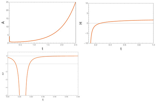
Figure 2. Phantom domination. This figure shows the time ($0.1\le t\le 2.5$) evolution of the scale factor $A\left(t\right)$, the Hubble parameter $H\left(t\right)$, and the barotropic parameter ${\omega }_{{\varphi }_1{\varphi }_2}\left(t\right)$. We use arbitrary units, namely, $V_1=V_2=1.0$, $r_1=1.5$, $r_2=0.9$, $q_1=q_2=0.1$, $a_3=-6.0$, ${\lambda }_2=\sqrt{2}$, and ${\lambda }_1=6/{\lambda }_2$. The remaining constants can be obtained from the aforementioned values. Note that time is measured in reduced Planck units since $8\pi G=1$.

2.1.4. Quintessence Domination: ${\lambda }_1<\sqrt{6}$ and ${\lambda }_2>\sqrt{6}$

We reinsert the solutions of ${\lambda }_1<\sqrt{6}$ (${\eta }_1>0$) and ${\lambda }_2>\sqrt{6}$ into the Hamilton equations for the momenta, leading to

$$\begin{array}{ccc}\hfill P_1& =& p_1-\frac{r_1}{12{\eta }_1}Coth\left(r_{1}t-q_1\right),\hfill \end{array}$$

(56)

$$\begin{array}{ccc}\hfill P_2& =& p_2-\frac{r_2}{12{\eta }_2}Coth\left(r_{2}t-q_2\right),\hfill \end{array}$$

(57)

where $p_1$ and $p_2$ are integration constants. We use (56) and (57) to obtain a null Hamiltonian when

$$p_1=\frac{{\eta }_1-9}{{\eta }_1}{p}_3,p_2=\frac{{\eta }_2-9}{{\eta }_2}{p}_3,p_3=\pm \frac{1}{36}\sqrt{\frac{{\eta }_2{r}_1^2+{\eta }_1{r}_2^2}{3\left[3{\eta }_1+3{\eta }_2-{\eta }_1{\eta }_2\right]}}.$$

(58)

As a consequence, the solutions of ${\xi }_i$ take the following form:

$$\begin{array}{cc}\hfill {\xi }_1& =Ln\left(\frac{r_1^2}{288{\eta }_1{V}_1}\right)+Ln\left[Csc{h}^2\left(r_{1}t-q_1\right)\right],\hfill \end{array}$$

(59)

$$\begin{array}{cc}\hfill {\xi }_2& =Ln\left(\frac{r_2^2}{288{\eta }_2{V}_2}\right)+Ln\left[Csc{h}^2\left(r_{2}t-q_2\right)\right],\hfill \end{array}$$

(60)

$$\begin{array}{cc}\hfill {\xi }_3& =a_3-648\frac{-{\eta }_1{\eta }_2+3{\eta }_1+3{\eta }_2}{{\eta }_1{\eta }_2}{p}_{3}t+\frac{{\eta }_1-9}{{\eta }_1}Ln\left[Sin{h}^2\left(r_{1}t-q_1\right)\right]\hfill \\ \hfill & +\frac{{\eta }_2-9}{{\eta }_2}Ln\left[Sin{h}^2\left(r_{2}t-q_2\right)\right],\hfill \end{array}$$

(61)

with an integration constant $a_3$. Then, we apply the inverse transformation (26) to arrive at the solutions in terms of the original variables, which read $\begin{array}{cc}\hfill \Omega & =Ln{\left[\frac{r_1{r}_2}{288\sqrt{{\eta }_1{\eta }_2{V}_1{V}_2}}\right]}^{\frac{1}{9}}+\frac{a_3}{18}+Ln\left[Csc{h}^{{\beta }_1}\left(r_{1}t-q_1\right)Csc{h}^{{\beta }_2}\left(r_{2}t-q_2\right)\right]\hfill \\ \hfill & -36\frac{3{\eta }_1+3{\eta }_2-{\eta }_1{\eta }_2}{{\eta }_1{\eta }_2}{p}_{3}t,\hfill \\ \hfill {\varphi }_1& ={\varphi }_{10}+Ln\left[Cos{h}^{\frac{2\left(|{\eta }_1|+3\right)}{{\lambda }_1\left|{\eta }_1\right|}}\left(r_{1}t-q_1\right)Csc{h}^{\frac{6}{{\lambda }_1{\eta }_2}}\left(r_{2}t-q_2\right)\right]+216\frac{|{\eta }_1|{\eta }_2-3\left|{\eta }_1\right|+3{\eta }_2}{{\lambda }_1\left|{\eta }_1\right|{\eta }_2}{p}_{3}t,\hfill \\ \hfill {\varphi }_2& ={\varphi }_{20}+Ln\left[Cos{h}^{\frac{6}{{\lambda }_2\left|{\eta }_1\right|}}\left(r_{1}t-q_1\right)Sin{h}^{\frac{2\left({\eta }_2-3\right)}{{\lambda }_2{\eta }_2}}\left(r_{2}t-q_2\right)\right]\hfill \\ \hfill & +216\frac{|{\eta }_1|{\eta }_2-3\left|{\eta }_1\right|+3{\eta }_2}{{\lambda }_2\left|{\eta }_1\right|{\eta }_2}{p}_{3}t,\hfill \end{array}$ where ${\beta }_1=1/{\eta }_1$, ${\beta }_2=1/{\eta }_2$, and the constants ${\Omega }_0,{\varphi }_{10}$, and ${\varphi }_{20}$ are those in (54). With these solutions, we can write the scale factor in the following form:

$$\begin{array}{cc}\hfill A\left(t\right)& ={\left[\frac{r_1{r}_2}{288\sqrt{{\eta }_1{\eta }_2{V}_1{V}_2}}\right]}^{\frac{1}{9}}{e}^{\frac{a_3}{18}}Csc{h}^{{\beta }_1}\left(r_{1}t-q_1\right)Csc{h}^{{\beta }_2}\left(r_{2}t-q_2\right)\hfill \\ \hfill & \times Exp\left[-36\frac{3{\eta }_1+3{\eta }_2-{\eta }_1{\eta }_2}{{\eta }_1{\eta }_2}{p}_{3}t\right].\hfill \end{array}$$

(62)

Immediately, one can observe that to obtain an increasing scale factor with respect to time, the constant $p_3$ must be negative. However, none of the parameters considered in this scenario lead to $p_3<0$; therefore, this solution is not physically relevant.

3. Quantum Formalism

To present the quantum mechanical version of the classical model, in (25) we promote the classical momenta to operators making the replacement ${\Pi }_{q^{\mu }}=-i\hslash {\partial }_{q^{\mu }}$, obtaining the following Hamiltonian density:

$$\mathcal{H}={\Pi }_{\Omega }^2+Qi\hslash {\Pi }_{\Omega }-12{\Lambda }_2{\Pi }_{{\varphi }_1}^2+12{\Lambda }_1{\Pi }_{{\varphi }_2}^2-24{\Lambda }_0{\Pi }_{{\varphi }_1}{\Pi }_{{\varphi }_2}-24V_1{e}^{-{\lambda }_1{\varphi }_1+6\Omega }-24V_2{e}^{-{\lambda }_2{\varphi }_2+6\Omega }.$$

(63)

To obtain Equation (63), we have substituted $e^{-3\Omega }{\Pi }_{\Omega }^2\to e^{-3\Omega }\left[{\Pi }_{\Omega }^2+Qi\hslash {\Pi }_{\Omega }\right]$ since one has to take into account the factor-ordering problem between the $e^{-3\Omega }$ and its momentum ${\Pi }_{\Omega }$; hence, Q is a number that measures such ambiguity. In order to have a more manageable functional form of (63), we take the constraint of the matrix element $m^{12}$ (Equation (30)); then, we apply the canonical transformation on variables $(\Omega ,{\varphi }_1,{\varphi }_2)\leftrightarrow ({\xi }_1,{\xi }_2,{\xi }_3)$ (Equations (26) and (27)), as well as the gauge $N=24e^{3\Omega }$. Therefore, we obtain

$$\begin{array}{cc}\hfill \mathcal{H}& =12{\eta }_1{P}_1^2+12{\eta }_2{P}_2^2+12\left(-9+{\eta }_1+{\eta }_2\right)P_3^2\hfill \\ \hfill & +24P_3\left[\left(9-{\eta }_1\right)P_1+\left(9-{\eta }_2\right)P_2\right]+6Qi\hslash \left(P_1+P_2+P_3\right)-24\left(V_1{e}^{{\xi }_1}+V_2{e}^{{\xi }_2}\right),\hfill \end{array}$$

(64)

with ${\eta }_1=3-{\Lambda }_1$ and ${\eta }_2=3+{\Lambda }_2$. Recall that the Hamiltonian density is identically zero $\mathcal{H}=0$; hence, the quantum counterpart of (64) is obtained by applying the same prescription used to obtain (63). Having this at hand, we can write down the Wheeler–DeWitt (WDW) equation, which reads

$$\begin{array}{cc}\hfill \widehat{\mathcal{H}}\Psi \left({\xi }_i\right)& =-12{\hslash }^2{\eta }_1\frac{{\partial }^2\Psi }{\partial {\xi }_1^2}-12{\hslash }^2{\eta }_2\frac{{\partial }^2\Psi }{\partial {\xi }_2^2}-12{\hslash }^2\left(-9+{\eta }_1+{\eta }_2\right)\frac{{\partial }^2\Psi }{\partial {\xi }_3^2}\hfill \\ \hfill & +6Q{\hslash }^2\left(\frac{\partial \Psi }{\partial {\xi }_1}+\frac{\partial \Psi }{\partial {\xi }_2}+\frac{\partial \Psi }{\partial {\xi }_3}\right)-{\hslash }^{2}24\left[\left(9-{\eta }_1\right)\frac{{\partial }^2\Psi }{\partial {\xi }_1\partial {\xi }_3}+\left(9-{\eta }_2\right)\frac{{\partial }^2\Psi }{\partial {\xi }_2\partial {\xi }_3}\right]\hfill \\ \hfill & -24\left(V_1{e}^{{\xi }_1}+V_2{e}^{{\xi }_2}\right)\Psi =0.\hfill \end{array}$$

(65)

In order to solve the WDW equation, we propose the following solution for the wave function $\Psi ({\xi }_1,{\xi }_2,{\xi }_3)=e^{p_3{\xi }_3}\mathcal{G}({\xi }_1,{\xi }_2)$ with $p_3=constant$. Additionally, we take as an ansatz $\mathcal{G}({\xi }_1,{\xi }_2)=G_1\left({\xi }_1\right)G_2\left({\xi }_2\right)$; upon substitution in (65), we obtain the following.

$$\begin{array}{cc}\hfill & -12{\eta }_1{G}_2\frac{{\partial }^2{G}_1}{\partial {\xi }_1^2}+6\left(Q-4p_3(9-{\eta }_1)\right)G_2\frac{\partial G_1}{\partial {\xi }_1}\hfill \\ \hfill & +3\left[p_3\left(Q-2p_3(9-{\eta }_1+{\eta }_2)\right)-8\frac{V_1}{{\hslash }^2}{e}^{{\xi }_1}\right]G_1{G}_2+\hfill \\ \hfill & -12{\eta }_2{G}_1\frac{{\partial }^2{G}_2}{\partial {\xi }_2^2}+6\left(Q-4p_3(9-{\eta }_2)\right)G_1\frac{\partial G_2}{\partial {\xi }_2}\hfill \\ \hfill & +3\left[p_3\left(Q-2p_3(9-{\eta }_1+{\eta }_2)\right)-8\frac{V_2}{{\hslash }^2}{e}^{{\xi }_2}\right]G_1{G}_2=0,\hfill \end{array}$$

(66)

finally, we factorize $G_1{G}_2$. Thus, two ordinary differential equations for the functions $G_1$ and $G_2$ emerge

$$\begin{array}{c}-12\frac{{\eta }_1}{G_1}\frac{{\partial }^2{G}_1}{\partial {\xi }_1^2}+6\left(Q-4p_3(9-{\eta }_1)\right)\frac{1}{G_1}\frac{\partial G_1}{\partial {\xi }_1}\hfill \\ \hspace{1em}\hspace{1em}\hspace{1em}\hspace{1em}\hspace{1em}\hspace{1em}\hspace{1em}\hspace{1em}\hspace{1em}\hspace{1em}\hspace{1em}+3\left[p_3\left(Q-2p_3(9-{\eta }_1+{\eta }_2)\right)-8\frac{V_1}{{\hslash }^2}{e}^{{\xi }_1}\right]-{\nu }^2=0,\hfill \end{array}$$

(67)

$$\begin{array}{c}-12\frac{{\eta }_2}{G_2}\frac{{\partial }^2{G}_2}{\partial {\xi }_2^2}+6\left[Q-4p_3(9-{\eta }_2)\right]\frac{1}{G_2}\frac{\partial G_2}{\partial {\xi }_2}\hfill \\ \hspace{1em}\hspace{1em}\hspace{1em}\hspace{1em}\hspace{1em}\hspace{1em}\hspace{1em}\hspace{1em}\hspace{1em}\hspace{1em}+3\left[p_3\left(Q-2p_3(9-{\eta }_1+{\eta }_2)\right)-8\frac{V_2}{{\hslash }^2}{e}^{{\xi }_2}\right]+{\nu }^2=0,\hfill \end{array}$$

(68)

where ${\nu }^2$ is an arbitrary constant. These last two equations can be written as $y^{″}+a{y}^{\prime }+\left(b{e}^{\kappa x}+c\right)y=0$, and their solutions are of the form [67]

$$Y\left(x\right)=Exp\left(-\frac{ax}{2}\right)Z_{\rho }\left(\frac{2\sqrt{b}}{\kappa }{e}^{\frac{\kappa x}{2}}\right),$$

(69)

here, $Z_{\rho }$ are the generic Bessel functions with the order $\rho =\sqrt{a^2-4c}/\kappa$. If $\sqrt{b}$ is real, $Z_{\rho }$ becomes the ordinary Bessel function; otherwise, the solutions will be given in terms of the modified Bessel functions. In the next sections, we will show quantum solutions separated into two classes, according to ${\eta }_1$ and ${\lambda }_1{\lambda }_2=6$.

3.1. Quantum Solution for ${\eta }_1>0$ and ${\lambda }_1<\sqrt{6}$

First, we identify the following expressions for Equation (67):

$$\begin{array}{ccc}\hfill \kappa & =& 1,a=-\frac{Q-4p_3(9-{\eta }_1)}{2{\eta }_1},\hfill \\ \hfill b& =& \frac{2V_2}{{\eta }_1{\hslash }^2},c=-\frac{p_3\left[Q-2p_3(9-{\eta }_1+{\eta }_2)\right]}{4{\eta }_1}+\frac{{\nu }^2}{12{\eta }_1},\hfill \end{array}$$

(70)

and for (68)

$$\begin{array}{ccc}\hfill \kappa & =& 1,a=-\frac{Q-4p_3(9-{\eta }_2)}{2{\eta }_2},\hfill \\ \hfill b& =& \frac{2V_1}{{\eta }_2{\hslash }^2},c=-\frac{p_3\left[Q-2p_3(9-{\eta }_1+{\eta }_2)\right]}{4{\eta }_2}-\frac{{\nu }^2}{12{\eta }_2}.\hfill \end{array}$$

(71)

Note that in both cases, $\sqrt{b}$ is real; then, the solutions are written in terms of the ordinary Bessel functions $Z_{{\rho }_i}=J_{{\rho }_i}$. Thus, the wave function becomes the following:

$${\mathcal{B}}_{{\rho }_1{\rho }_2}={\mathcal{B}}_0{J}_{{\rho }_1}\left[\frac{2}{\hslash }\sqrt{\frac{2V_1}{{\eta }_1}}{e}^{\frac{{\xi }_1}{2}}\right]J_{{\rho }_2}\left[\frac{2}{\hslash }\sqrt{\frac{2V_2}{{\eta }_2}}{e}^{\frac{{\xi }_2}{2}}\right]e^{\theta },$$

where

$$\theta =\frac{Q-4p_3(9-{\eta }_1)}{4{\eta }_1}{\xi }_1+\frac{Q-4p_3(9-{\eta }_2)}{4{\eta }_2}{\xi }_2,$$

and ${\mathcal{B}}_0$ is an integration constant. Additionally, the order of the two Bessel functions are

$$\begin{array}{ccc}& & {\rho }_1=\sqrt{{\left(-\frac{Q-4p_3(9-{\eta }_1)}{2{\eta }_1}\right)}^2+\frac{p_3(Q-2p_3(9-{\eta }_1+{\eta }_2))}{{\eta }_1}-\frac{{\nu }^2}{3{\eta }_1}},\hfill \end{array}$$

(72)

$$\begin{array}{ccc}& & {\rho }_2=\sqrt{{\left(-\frac{Q-4p_3(9-{\eta }_2)}{2{\eta }_2}\right)}^2+\frac{p_3(Q-2p_3(9-{\eta }_1+{\eta }_2))}{{\eta }_2}+\frac{{\nu }^2}{3{\eta }_2}}.\hfill \end{array}$$

(73)

Hence, the wave function $\Psi$ in the original variables becomes

$${\Psi }_{{\rho }_1{\rho }_2}={\Psi }_0{A}^{6\alpha }Exp\left[{\alpha }_1{\lambda }_1{\varphi }_1+{\alpha }_2{\lambda }_2{\varphi }_2\right]J_{{\rho }_1}\left[\frac{2}{\hslash }\sqrt{\frac{2V_1}{{\eta }_1}}{A}^3{e}^{\frac{-{\lambda }_1{\varphi }_1}{2}}\right]J_{{\rho }_2}\left[\frac{2}{\hslash }\sqrt{\frac{2V_2}{{\eta }_2}}{A}^3{e}^{-\frac{{\lambda }_2{\varphi }_2}{2}}\right],$$

(74)

where ${\Psi }_0$ is a normalization constant, and

$$\begin{array}{ccc}& & \alpha =\frac{Q({\eta }_2+{\eta }_1)}{4{\eta }_1{\eta }_2}-\frac{p_3(9-{\eta }_1)}{{\eta }_1}-\frac{p_3(9-{\eta }_2)}{{\eta }_2}+p_3,\hfill \\ & & {\alpha }_1=-\frac{Q-4p_3(9-{\eta }_1)}{4{\eta }_1}+p_3,{\alpha }_2=-\frac{Q-4p_3(9-{\eta }_2)}{4{\eta }_2}+p_3.\hfill \end{array}$$

(75)

By analyzing solution (74), we could not find any set of parameter values for which the probability density function (defined by the wave function (74)) is bounded. This unwanted behavior prevents us from directly implementing the standard interpretation of quantum mechanics in order to draw meaningful physical conclusions. This setback is tempered by the fact that the corresponding classical solution (given essentially by (62)) is not of physical relevance, and so no further analysis will be performed regarding this case.

3.2. Quantum Solution When ${\eta }_1<0$ and ${\lambda }_1>\sqrt{6}$

We set up the corresponding parameters for Equation (67)

$$\begin{array}{ccc}\hfill \kappa & =& 1a=\frac{Q-4p_3(9+|{\eta }_1\left|\right)}{2|{\eta }_1|},\hfill \\ \hfill b& =& -\frac{2V_2}{|{\eta }_1|{\hslash }^2}c=\frac{p_3\left[Q-2p_3(9+|{\eta }_1|+{\eta }_2)\right]}{4|{\eta }_1|}-\frac{{\nu }^2}{12|{\eta }_1|},\hfill \end{array}$$

(76)

and for (68)

$$\begin{array}{ccc}\hfill \kappa & =& 1a=-\frac{Q-4p_3(9-{\eta }_2)}{2{\eta }_2},\hfill \\ \hfill b& =& \frac{2V_1}{{\eta }_2{\hslash }^2},c=-\frac{p_3\left[Q-2p_3(9+|{\eta }_1|+{\eta }_2)\right]}{4{\eta }_2}-\frac{{\nu }^2}{12{\eta }_2},\hfill \end{array}$$

(77)

note that we have inverted the sign of the previous formulas. Hereby, we introduce $|{\eta }_1|$. Then, the first case (76) yields an imaginary $\sqrt{b}$; therefore, its solution must be in terms of the modified Bessel function $Z_{{\rho }_1}=K_{{\rho }_1}$ (contrary to the second case, where the proper function is $Z_{{\rho }_2}=J_{{\rho }_2}$). Hence, we have

$${\mathcal{B}}_{{\rho }_1{\rho }_2}={\mathcal{B}}_0{K}_{{\rho }_1}\left[\frac{2}{\hslash }\sqrt{\frac{2V_1}{|{\eta }_1|}}{e}^{\frac{{\xi }_1}{2}}\right]J_{{\rho }_2}\left[\frac{2}{\hslash }\sqrt{\frac{2V_2}{{\eta }_2}}{e}^{\frac{{\xi }_2}{2}}\right]e^{{\theta }_2},$$

(78)

here

$${\theta }_2=-\frac{Q-4p_3(9+|{\eta }_1\left|\right)}{4|{\eta }_1|}{\xi }_1+\frac{Q-4p_3(9-{\eta }_2)}{4{\eta }_2}{\xi }_2,$$

(79)

and the order of both Bessel functions are

$$\begin{array}{ccc}& & {\rho }_1=\sqrt{{\left(\frac{Q-4p_3(9+|{\eta }_1|}{2|{\eta }_1|}\right)}^2-\frac{p_3(Q-2p_3(9+|{\eta }_1|+{\eta }_2\left)\right)}{|{\eta }_1|}+\frac{{\nu }^2}{3|{\eta }_1|}},\hfill \end{array}$$

(80)

$$\begin{array}{ccc}& & {\rho }_2=\sqrt{{\left(-\frac{Q-4p_3(9-{\eta }_2}{2{\eta }_2}\right)}^2+\frac{p_3(Q-2p_3(9+|{\eta }_1|+{\eta }_2\left)\right)}{{\eta }_2}+\frac{{\nu }^2}{3{\eta }_2}}.\hfill \end{array}$$

(81)

Finally, the wave function in the original variables is given by

$${\Psi }_{{\rho }_1{\rho }_2}={\Psi }_0{A}^{6\beta }Exp\left[{\alpha }_1{\lambda }_1{\varphi }_1+{\alpha }_2{\lambda }_2{\varphi }_2\right]K_{{\rho }_1}\left[\frac{2}{\hslash }\sqrt{\frac{2V_1}{|{\eta }_1|}}{A}^3{e}^{\frac{-{\lambda }_1{\varphi }_1}{2}}\right]J_{{\rho }_2}\left[\frac{2}{\hslash }\sqrt{\frac{2V_2}{{\eta }_2}}{A}^3{e}^{-\frac{{\lambda }_2{\varphi }_2}{2}}\right],$$

(82)

where

$$\begin{array}{ccc}& & \beta =-\frac{Q({\eta }_2-|{\eta }_1\left|\right)}{4|{\eta }_1|{\eta }_2}+\frac{p_3(9+|{\eta }_1\left|\right)}{|{\eta }_1|}-\frac{p_3(9-{\eta }_2)}{{\eta }_2}+p_3,\hfill \end{array}$$

(83)

$$\begin{array}{ccc}& & {\alpha }_1=\frac{Q-4p_3(9+|{\eta }_1\left|\right)}{4|{\eta }_1|}+p_3,{\alpha }_2=-\frac{Q-4p_3(9-{\eta }_2)}{2{\eta }_2}+p_3,\hfill \end{array}$$

(84)

and a normalization constant ${\Psi }_0$. The behaviour of the probability density can be seen in Figure 3. Observe that in all panels, the probability density dies away as the scale factor and scalar field evolve, an expected outcome already reported in [68,69,70]. On the other hand, we vary the factor ordering constant Q, in order to show how ${|\Psi |}^2$ behaves. We can see that whilst $Q\ll 0$, the probability density tends to the phantom sector. In [68], the authors showed that the parameter Q acts a retarder of the wave function and compresses the length on the axis where the field evolves; however, they analysed the case of two quintessence fields.

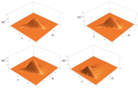
Figure 3. Phantom scenario. These figures show the probability density of the wave function (82) for the values of $Q=2$ and $Q=0$ (top panels from left to right, respectivley), and $Q=-2$ and $Q=-4$ (bottom panels from left to right, respectively). We use arbitrary units, namely, $\nu =10$, ${\lambda }_1=10.5$, ${\lambda }_2=6/{\lambda }_1$, $V_1=0.1, V_2={10}^{-5}$, $r_1=49$, $r_2=1.5, a_3=-2.3$, and $p_3=0.326878$, and the bounce in the quintessence field ${\varphi }_1=1.455$. The remaining constants can be obtained from the aforementioned values. Additionally, for $Q=2,0$ we take ${\Psi }_0={10}^{-3}, {10}^{-2}$ respectively; then, for $Q=-2, -4$ we chose ${\Psi }_0={10}^{-1}, 1/\sqrt{10}$ respectively. Note that the probability density tends toward the phantom sector when the factor ordering constant $Q\ll 0$.

3.3. Quantum Solution When ${\lambda }_1={\lambda }_2=\sqrt{6}$, Therefore ${\eta }_1=0$ and ${\eta }_2=6$

In this final case, we take ${\lambda }_1={\lambda }_2=\sqrt{6}$; therefore, ${\eta }_1=0$ and ${\eta }_2=6$. Hence, the Equations (67) and (68) can be reduced to

$$\begin{array}{cc}\hfill 6\left(Q-36p_3\right)\frac{1}{G_1}\frac{\partial G_1}{\partial {\xi }_1}+3\left[p_3\left(Q-30p_3\right)-8\frac{V_1}{{\hslash }^2}{e}^{{\xi }_1}\right]-{\nu }^2& =0,\hfill \end{array}$$

(85)

$$\begin{array}{cc}\hfill -\frac{72}{G_2}\frac{{\partial }^2{G}_2}{\partial {\xi }_2^2}+6\left[Q-12p_3\right]\frac{1}{G_2}\frac{\partial G_2}{\partial {\xi }_2}+3\left[p_3\left(Q-30p_3\right)-8\frac{V_2}{{\hslash }^2}{e}^{{\xi }_2}\right]+{\nu }^2& =0.\hfill \end{array}$$

(86)

The solution of (85) is given by

$$G_1=G_{0}Exp\left[\frac{\frac{{\nu }^2}{3}-p_3(Q-30p_3)}{2(Q-36p_3)}{\xi }_1+\frac{4V_1}{{\hslash }^2(Q-36p_3)}{e}^{{\xi }_1}\right],$$

(87)

where $G_0$ in an integration constant. Then, for $G_2$ we have the following ordinary Bessel function:

$$G_2=Exp\left[\frac{Q-12p_3}{24}{\xi }_2\right]J_{{\rho }_2}\left[\frac{\sqrt{V_2}}{\hslash }{e}^{\frac{{\xi }_2}{2}}\right],$$

(88)

here, the order is

$${\rho }_2=\sqrt{{\left(\frac{Q-12p_3}{12}\right)}^2+\frac{1}{6}\left[\frac{{\nu }^2}{3}+p_3(Q-30p_3)\right]}.$$

(89)

Remarkably for this case, we can obtain a parameter space of $Q,\nu$, and $p_3$ where the order can be real or imaginary. Hence, we have

$$\mathcal{B}={\mathcal{B}}_0{J}_{{\rho }_2}\left[\frac{\sqrt{V_2}}{\hslash }{e}^{\frac{{\xi }_2}{2}}\right]e^{{\theta }_3},$$

(90)

with

$${\theta }_3=\frac{\frac{{\nu }^2}{3}-p_3(Q-30p_3)}{2(Q-36p_3)}{\xi }_1+\frac{Q-12p_3}{24}{\xi }_2+\frac{4V_1}{{\hslash }^2(Q-36p_3)}{e}^{{\xi }_1},$$

Finally, in the original variables the wave function is

$$\Psi ={\psi }_0{A}^{6\eta }{J}_{{\rho }_2}\left[\frac{\sqrt{V_2}}{\hslash }{A}^3{e}^{\frac{-{\lambda }_2{\varphi }_2}{2}}\right]e^{{\theta }_1},$$

(91)

where

$${\theta }_1=\frac{4V_1}{{\hslash }^2(Q-36p_3)}{A}^6{e}^{-{\lambda }_1{\varphi }_1}+{\alpha }_1{\lambda }_1{\varphi }_1+{\alpha }_2{\lambda }_2{\varphi }_2,$$

(92)

and

$$\begin{array}{ccc}& & \eta =\frac{\frac{{\nu }^2}{3}-p_3(Q-30p_3)}{2(Q-36p_3)}+\frac{Q-12p_3}{24}+p_3\hfill \\ & & {\alpha }_1=-\frac{\frac{{\nu }^2}{3}-p_3(Q-30p_3)}{2(Q-36p_3)}+p_3,{\alpha }_2=-\frac{Q-12p_3}{24}+p_3,\hfill \end{array}$$

(93)

and a normalization constant ${\psi }_0$. For completeness of the above classical solutions, we include this case; however, once more the probability density function is not bounded since ${|\Psi |}^2$ does not fade as the scale factor and scalar field evolve. We recall that the standard interpretation of quantum mechanics becomes troublesome to realize due to this nuisance behavior. Therefore, the wave function (91) is not physically relevant.

4. Final Remarks

In this work, we have studied a chiral cosmological model from the point of view of a K-essence formalism. The background geometry was a flat FLRW universe minimally coupled to quintom fields: one quintessence and one phantom. In this approach, the scalar fields interact within the kinetic and potential sectors.

In the classical framework, we established the Hamiltonian density (31), which in turn allows one to find exact solutions for different sets of values of the free parameters. We highlight two cases: the first when ${\lambda }_1={\lambda }_2=\sqrt{6}$, and the second where phantom domination is the relevant factor, namely, ${\lambda }_1>\sqrt{6}$ and ${\lambda }_2<\sqrt{6}$. In the two scenarios, the scale factor grows very rapidly and the big-bang singularity is avoided via a bounce. We call it the “big bounce”. In fact, this claim is also supported by the behavior of both the scale factor and the Hubble parameter. Finally, we show that the barotropic parameter is capable of transiting from a quintessence phase to a phantom one, i.e., it crosses the phantom divide line. In Figure 1 and Figure 2, we show the behavior of these quantities as a function of time.

On the other hand, using the canonical quantization procedure, we were able to establish the quantum counterpart of the classical model and compute the Wheeler–DeWitt equation. Once again, we solve it for various scenarios given by different sets of values of the free parameters. In particular, we found exact solutions for three distinct cases: ${\eta }_1>0$ and ${\lambda }_1<\sqrt{6}$, ${\eta }_1<0$ and ${\lambda }_1>\sqrt{6}$, and ${\lambda }_1={\lambda }_2=\sqrt{6}$; therefore, ${\eta }_1=0$ and ${\eta }_2=6$. Figure 3 shows the behavior of the probability density as a function of the scale factor and scalar field, for the phantom case, i.e., ${\eta }_1<0$ and ${\lambda }_1>\sqrt{6}$. The probability density exhibits a damped behavior as the scale factor and scalar fields evolve. An expected result has already been reported in [68,69,70]. Lastly, we note that by varying Q, specifically when $Q\ll 0$, the probability density evolves towards the phantom sector. This outcome contrasts with that reported in [68], where the authors showed that the parameter Q delays the evolution of the wave function and compresses the length on the axis where the field evolves; however, they analyzed the case of two quintessence fields.

References

- Perlmutter, S.; Aldering, G.; Goldhaber, G.; Knop, R.A.; Nugent, P.; Castro, P.G.; Couch, W.J. Measurements of Ω and Λ from 42 high redshift supernovae. Astrophys. J. 1999, 517, 565–586. [Google Scholar] [CrossRef]
- Riess, A.G.; Filippenko, A.V.; Challis, P.; Clocchiatti, A.; Diercks, A.; Garnavich, P.M.; Tonry, J. Observational evidence from supernovae for an accelerating universe and a cosmological constant. Astron. J. 1998, 116, 1009–1038. [Google Scholar] [CrossRef]
- Garnavich, P.M.; Kirshner, R.P.; Challis, P.; Tonry, J.; Gilliland, R.L.; Smith, R.C.; Wells, L. Constraints on cosmological models from Hubble Space Telescope observations of high z supernovae. Astrophys. J. Lett. 1998, 493, L53–L57. [Google Scholar] [CrossRef]
- Komatsu, E.; Dunkley, J.; Nolta, M.R.; Bennett, C.L.; Gold, B.; Hinshaw, G.; Wright, E.L. Five-Year Wilkinson Microwave Anisotropy Probe (WMAP) Observations: Cosmological Interpretation. Astrophys. J. Suppl. 2009, 180, 330–376. [Google Scholar] [CrossRef]
- Guth, A.H. The Inflationary Universe: A Possible Solution to the Horizon and Flatness Problems. Phys. Rev. D 1981, 23, 347–356. [Google Scholar] [CrossRef]
- Linde, A.D. A New Inflationary Universe Scenario: A Possible Solution of the Horizon, Flatness, Homogeneity, Isotropy and Primordial Monopole Problems. Phys. Lett. B 1982, 108, 389–393. [Google Scholar] [CrossRef]
- Copeland, E.J.; Sami, M.; Tsujikawa, S. Dynamics of dark energy. Int. J. Mod. Phys. D 2006, 15, 1753–1936. [Google Scholar] [CrossRef]
- Clifton, T.; Ferreira, P.G.; Padilla, A.; Skordis, C. Modified Gravity and Cosmology. Phys. Rept. 2012, 513, 1–189. [Google Scholar] [CrossRef]
- Nojiri, S.; Odintsov, S.D.; Oikonomou, V.K. Modified Gravity Theories on a Nutshell: Inflation, Bounce and Late-time Evolution. Phys. Rept. 2017, 692, 1–104. [Google Scholar] [CrossRef]
- Urena-Lopez, L.A.; Matos, T. A New cosmological tracker solution for quintessence. Phys. Rev. D 2000, 62, 081302. [Google Scholar] [CrossRef]
- Ratra, B.; Peebles, P.J.E. Cosmological Consequences of a Rolling Homogeneous Scalar Field. Phys. Rev. D 1988, 37, 3406. [Google Scholar] [CrossRef]
- Harko, T.; Lobo, F.S.N.; Mak, M.K. Arbitrary scalar field and quintessence cosmological models. Eur. Phys. J. C 2014, 74, 2784. [Google Scholar] [CrossRef]
- Rubano, C.; Barrow, J.D. Scaling solutions and reconstruction of scalar field potentials. Phys. Rev. D 2001, 64, 127301. [Google Scholar] [CrossRef]
- Sahni, V.; Starobinsky, A. The Case for a positive cosmological Lambda term. Int. J. Mod. Phys. D 2000, 9, 373–444. [Google Scholar] [CrossRef]
- Sahni, V.; Wang, L.M. A New cosmological model of quintessence and dark matter. Phys. Rev. D 2000, 62, 103517. [Google Scholar] [CrossRef]
- Paliathanasis, A.; Tsamparlis, M.; Basilakos, S.; Barrow, J.D. Dynamical analysis in scalar field cosmology. Phys. Rev. D 2015, 91, 123535. [Google Scholar] [CrossRef]
- Dimakis, N.; Karagiorgos, A.; Zampeli, A.; Paliathanasis, A.; Christodoulakis, T.; Terzis, P.A. General Analytic Solutions of Scalar Field Cosmology with Arbitrary Potential. Phys. Rev. D 2016, 93, 123518. [Google Scholar] [CrossRef]
- Fang, W.; Lu, H.Q.; Huang, Z.G.; Zhang, K.G. The evolution of the universe with the B-I type phantom scalar field. Int. J. Mod. Phys. D 2006, 15, 199–214. [Google Scholar] [CrossRef]
- Cataldo, M.; Arevalo, F.; Mella, P. Canonical and phantom scalar fields as an interaction of two perfect fluids. Astrophys. Space Sci. 2013, 344, 495–503. [Google Scholar] [CrossRef]
- Nojiri, S.; Odintsov, S.D.; Oikonomou, V.K.; Saridakis, E.N. Singular cosmological evolution using canonical and ghost scalar fields. JCAP 2015, 9, 044. [Google Scholar] [CrossRef]
- Cai, Y.F.; Saridakis, E.N.; Setare, M.R.; Xia, J.Q. Quintom Cosmology: Theoretical implications and observations. Phys. Rept. 2010, 493, 1–60. [Google Scholar] [CrossRef]
- Setare, M.R.; Saridakis, E.N. Quintom Cosmology with General Potentials. Int. J. Mod. Phys. D 2009, 18, 549–557. [Google Scholar] [CrossRef]
- Lazkoz, R.; Leon, G.; Quiros, I. Quintom cosmologies with arbitrary potentials. Phys. Lett. B 2007, 649, 103–110. [Google Scholar] [CrossRef]
- Leon, G.; Paliathanasis, A.; Morales-Martínez, J.L. The past and future dynamics of quintom dark energy models. Eur. Phys. J. C 2018, 78, 753. [Google Scholar] [CrossRef]
- Dimakis, N.; Paliathanasis, A. Crossing the phantom divide line as an effect of quantum transitions. Class. Quant. Grav. 2021, 38, 075016. [Google Scholar] [CrossRef]
- Elizalde, E.; Nojiri, S.; Odintsov, S.D.; Saez-Gomez, D.; Faraoni, V. Reconstructing the universe history, from inflation to acceleration, with phantom and canonical scalar fields. Phys. Rev. D 2008, 77, 106005. [Google Scholar] [CrossRef]
- Chervon, S.V. On the chiral model of cosmological inflation. Russ. Phys. J. 1995, 38, 539–543. [Google Scholar] [CrossRef]
- Chervon, S.V. Chiral Cosmological Models: Dark Sector Fields Description. Quant. Matt. 2013, 2, 71–82. [Google Scholar] [CrossRef]
- Christodoulidis, P.; Roest, D.; Sfakianakis, E.I. Scaling attractors in multi-field inflation. JCAP 2019, 12, 059. [Google Scholar] [CrossRef]
- Beesham, A.; Chervon, S.V.; Maharaj, S.D.; Kubasov, A.S. An Emergent Universe with Dark Sector Fields in a Chiral Cosmological Model. Quant. Matt. 2013, 2, 388–395. [Google Scholar] [CrossRef]
- Chervon, S.V.; Abbyazov, R.R.; Kryukov, S.V. Dynamics of Chiral Cosmological Fields in the Phantom-Canonical Model. Russ. Phys. J. 2015, 58, 597–605. [Google Scholar] [CrossRef]
- Fomin, I.V. The chiral cosmological models with two components. J. Phys. Conf. Ser. 2017, 918, 012009. [Google Scholar] [CrossRef]
- Fomin, I.V. Two-Field Cosmological Models with a Second Accelerated Expansion of the Universe. Moscow Univ. Phys. Bull. 2018, 73, 696–701. [Google Scholar] [CrossRef]
- Paliathanasis, A.; Leon, G.; Pan, S. Exact Solutions in Chiral Cosmology. Gen. Rel. Grav. 2019, 51, 106. [Google Scholar] [CrossRef]
- Scherrer, R.J. Purely kinetic k-essence as unified dark matter. Phys. Rev. Lett. 2004, 93, 011301. [Google Scholar] [CrossRef]
- Bandyopadhyay, A.; Gangopadhyay, D.; Moulik, A. The k-essence scalar field in the context of Supernova Ia Observations. Eur. Phys. J. C 2012, 72, 1943. [Google Scholar] [CrossRef]
- Armendariz-Picon, C.; Damour, T.; Mukhanov, V.F. K-inflation. Phys. Lett. B 1999, 458, 209–218. [Google Scholar] [CrossRef]
- Damour, T.; Esposito-Farese, G. Tensor multiscalar theories of gravitation. Class. Quant. Grav. 1992, 9, 2093–2176. [Google Scholar] [CrossRef]
- Horndeski, G.W. Second-order scalar-tensor field equations in a four-dimensional space. Int. J. Theor. Phys. 1974, 10, 363–384. [Google Scholar] [CrossRef]
- Deffayet, C.; Esposito-Farese, G.; Vikman, A. Covariant Galileon. Phys. Rev. D 2009, 79, 084003. [Google Scholar] [CrossRef]
- Coley, A.A.; van den Hoogen, R.J. The Dynamics of multiscalar field cosmological models and assisted inflation. Phys. Rev. D 2000, 62, 023517. [Google Scholar] [CrossRef]
- Peebles, P.J.E.; Ratra, B. The Cosmological Constant and Dark Energy. Rev. Mod. Phys. 2003, 75, 559–606. [Google Scholar] [CrossRef]
- Padmanabhan, T. Cosmological constant: The Weight of the vacuum. Phys. Rept. 2003, 380, 235–320. [Google Scholar] [CrossRef]
- Albrecht, A.; Bernstein, G.; Cahn, R.; Freedman, W.L.; Hewitt, J.; Hu, W.; Huth, J.; Kamionkowski, M.; Kolb, E.W.; Knox, L. Report of the Dark Energy Task Force. arXiv 2003, arXiv:astro-ph/0609591. [Google Scholar]
- Linder, E.V. Mapping the Cosmological Expansion. Rept. Prog. Phys. 2008, 71, 056901. [Google Scholar] [CrossRef]
- Frieman, J.; Turner, M.; Huterer, D. Dark Energy and the Accelerating Universe. Ann. Rev. Astron. Astrophys. 2008, 46, 385–432. [Google Scholar] [CrossRef]
- Caldwell, R.R.; Kamionkowski, M. The Physics of Cosmic Acceleration. Ann. Rev. Nucl. Part. Sci. 2009, 59, 397–429. [Google Scholar] [CrossRef]
- Wetterich, C. Cosmology and the Fate of Dilatation Symmetry. Nucl. Phys. B 1988, 302, 668–696. [Google Scholar] [CrossRef]
- Caldwell, R.R. A Phantom menace? Phys. Lett. B 2002, 545, 23–29. [Google Scholar] [CrossRef]
- Caldwell, R.R.; Kamionkowski, M.; Weinberg, N.N. Phantom energy and cosmic doomsday. Phys. Rev. Lett. 2003, 91, 071301. [Google Scholar] [CrossRef]
- Feng, B.; Wang, X.L.; Zhang, X.M. Dark energy constraints from the cosmic age and supernova. Phys. Lett. B 2005, 607, 35–41. [Google Scholar] [CrossRef]
- Vikman, A. Can dark energy evolve to the phantom? Phys. Rev. D 2005, 71, 023515. [Google Scholar] [CrossRef]
- Deffayet, C.; Pujolas, O.; Sawicki, I.; Vikman, A. Imperfect Dark Energy from Kinetic Gravity Braiding. JCAP 2010, 10, 26. [Google Scholar] [CrossRef]
- Chimento, L.P.; Forte, M.I.; Lazkoz, R.; Richarte, M.G. Internal space structure generalization of the quintom cosmological scenario. Phys. Rev. D 2009, 79, 043502. [Google Scholar] [CrossRef]
- Lindle, A.D. Hybrid inflation. Phys. Rev. D 1994, 49, 784. [Google Scholar]
- Copeland, E.J.; Liddle, A.R.; Lyth, D.H.; Stewart, E.D.; Wands, D. False vacuum inflation with Einstein gravity. Phys. Rev. D 1994, 49, 6410–6433. [Google Scholar] [CrossRef]
- Kim, S.A.; Liddle, A.R. Nflation: Multi-field inflationary dynamics and perturbations. Phys. Rev. D 2006, 74, 023513. [Google Scholar] [CrossRef]
- Socorro, J.; Núñez, O.E. Scalar potentials with Multi-scalar fields from quantum cosmology and supersymmetric quantum mechanics. Eur. Phys. J. Plus 2017, 132, 168. [Google Scholar] [CrossRef]
- Liddle, A.R.; Mazumdar, A.; Schunck, F.E. Assisted inflation. Phys. Rev. D 1998, 58, 061301. [Google Scholar] [CrossRef]
- Copeland, E.J.; Mazumdar, A.; Nunes, N.J. Generalized assisted inflation. Phys. Rev. D 1999, 60, 083506. [Google Scholar] [CrossRef]
- Yokoyama, S.; Suyama, T.; Tanaka, T. Primordial Non-Gaussianity in Multi-Scalar Inflation. Phys. Rev. D 2008, 77, 083511. [Google Scholar] [CrossRef]
- Chiba, T.; Yamaguchi, M. Extended Slow-Roll Conditions and Primordial Fluctuations: Multiple Scalar Fields and Generalized Gravity. JCAP 2009, 901, 19. [Google Scholar] [CrossRef][Green Version]
- Socorro, J.; Pimentel, L.O.; Espinoza-García, A. Classical Bianchi type I cosmology in K-essence theory. Adv. High Energy Phys. 2014, 2014, 805164. [Google Scholar] [CrossRef]
- Chervon, S.V.; Fomin, I.V.; Pozdeeva, E.O.; Sami, M.; Vernov, S.Y. Superpotential method for chiral cosmological models connected with modified gravity. Phys. Rev. D 2019, 100, 063522. [Google Scholar] [CrossRef]
- Fomin, I.V.; Chervon, S.V. New method of exponential potentials reconstruction based on given scale factor in phantonical two-field models. arXiv 2021, arXiv:2112.09359. [Google Scholar] [CrossRef]
- Tot, J.; Yildirim, B.; Coley, A.; Leon, G. The dynamics of scalar-field quintom cosmological models. arXiv 2022, arXiv:2204.06538. [Google Scholar] [CrossRef]
- Zaitsev, V.F.; Polyanin, A.D. Handbook of Exact Solutions for Ordinary Differential Equations, 2nd ed.; Chapman & Hall/CRC: London, UK, 2003. [Google Scholar]
- Socorro, J.; Pérez-Payán, S.; Hernández-Jiménez, R.; Espinoza-García, A.; Díaz-Barrón, L.R. Classical and quantum exact solutions for a FRW in chiral like cosmology. Class. Quant. Grav. 2021, 38, 135027. [Google Scholar] [CrossRef]
- Socorro, J.; Núñez, O.E.; Hernández-Jiménez, R. Classical and quantum exact solutions for the anisotropic Bianchi type I in multi-scalar field cosmology with an exponential potential driven inflation. Phys. Lett. B 2020, 809, 135667. [Google Scholar] [CrossRef]
- Socorro, J.; Núñez, O.E.; Hernández-Jiménez, R. Classical and Quantum Exact Solutions for a FRW Multiscalar Field Cosmology with an Exponential Potential Driven Inflation. Adv. Math. Phys. 2018, 2018, 3468381. [Google Scholar] [CrossRef]
Publisher’s Note: MDPI stays neutral with regard to jurisdictional claims in published maps and institutional affiliations. |
© 2022 by the authors. Licensee MDPI, Basel, Switzerland. This article is an open access article distributed under the terms and conditions of the Creative Commons Attribution (CC BY) license (https://creativecommons.org/licenses/by/4.0/).