Abstract
We have analyzed the distribution of early-type galaxies (ETGs) in the effective surface intensity vs. effective radius () plane and in the total luminosity vs. central stellar velocity dispersion () diagram, with the aim of studying the physical variables that allow the transformation of one space-parameter into the other. We find that the classical Faber–Jackson relation , in which the parameters and are confined in a small range of possible values, is incompatible with the distribution observed in the plane. The two distributions become mutually consistent only if luminosity is not considered a pure proxy of mass but a variable tightly dependent on the past history of mass assembling and star formation and on the present evolutionary state of the stellar content of a galaxy. The solution comes by considering the law proposed by D’Onofrio et al. in 2020, in which both and can vary considerably from galaxy to galaxy. We will also show that the data of the Illustris numerical simulation prove the physical foundation of the law and confirm the prediction of the Zone of Exclusion (ZoE) originating from the intersection of the virial law with the relation. The ZoE is the region in the and diagrams avoided by real galaxies, and the border of which marks the condition of ‘full’ virial equilibrium with no recent significant merger events and no undergoing star formation.
1. Introduction
The scaling relations (SRs) are the chief tool at our disposal to decipher the physical properties of galaxies and their past history of formation and evolution. They are often represented by mathematical expressions that are fit of observed distributions in a parameters space. The most famous SRs generally involve the structural parameters of galaxies, such as the effective radius (, enclosing half the total luminosity), the mean effective surface intensity ()1 inside , the central velocity dispersion of stars (), and the total luminosity in a given pass-band ().
Although the body of the SRs is widely used, there are still points of uncertainty and even mutual contradictions that are not fully understood that we try to alleviate in this study. A typical example is provided by the SRs that involve the total luminosity L as a parameter (either explicitly or implicitly involved). At variance with mass, luminosity is a parameter that brings in the statistical correlations an intrinsic “degeneracy”, being closely related with and in the relation . This implies that a big number of combinations of and might belong to objects with the same luminosity. In addition, luminosity might increase/decrease for different reasons related to the star formation activity and/or the mass accumulation/stripping during merger events and the passive stellar evolution. This makes L a parameter that is not a simple proxy of mass but conceals the non-linear history of a galaxy growth. Consequently, in some SRs, luminosity enters simply as a proxy of mass, while in others, it displays its full physical background.
The most famous example is that of the “tilt” of the Fundamental Plane (FP), i.e., the planar distribution of ETGs observed in the space [1,2]. In that problem the use of the total luminosity instead of the total mass determines the well known ‘tilt’ of the plane with respect to the virial prediction. It is widely known that such a correlation contains a lot of information about galaxies’ evolution, such as, e.g., the systematic variation of the mass-to-light ratio with mass, the universality of the initial mass function, the role of metallicity, the amount and distribution of dark matter, etc.
Here, we want to recall two other milestone relationships that are still controversial and show a very different behavior of the ETGs despite both involving the total luminosity: the and relations.
The distribution of galaxies in the parameter space formed by effective radius and effective surface intensity inside this radius , otherwise known as the plane, was discovered by Kormendy in 1977 [3]. He found a log-linear relation with a slope ∼3 (when is expressed in units, and ∼−1.5 when in units) between these parameters using a sample of bright ETGs. As soon as new data for faint ETGs and late-type galaxies (LTGs) became available, the observed linear distribution started to show an ample curvature, clearly separating faint and dwarf objects with respect to bright ETGs [4]. Today, we know that the space is an orthogonal projection of the FP, and it is the most easily accessible correlation of galaxies parameters at low and high redshift.
The peculiar distribution observed in the plane suggested the existence of two different populations of ETGs, the ‘ordinary’ and the ‘bright’, which follow two different trends in this space. The ‘ordinary’ family is bi-parametric (), and its members are fainter than ∼, while their radii are smaller than ∼3 kpc. The ‘bright’ family is mono-parametric ( depends only on ), as it hosts only the brightest cluster galaxies (BCGs), and their members have radii larger than kpc. The spiral galaxies and their bulges belong to the ‘ordinary’ family and are not visible in the ‘bright’ sequence (see [4,5]).
This curved distribution has been used to argue for distinct channels of formation for dwarfs and giants ETGs (see, e.g., [6,7,8,9,10,11]). Many authors believe that there are two distinct kinds of ETGs, whose properties differ mainly for the different history of merging events, in particular for the characteristics of the last major mergers, wet or dry, according to whether cold gas dissipation and starbursts occurred or not. However, the existence of two physically distinct families of ETGs is not universally accepted. Many researchers advocated for a continuity among the ETG population [12,13,14,15]. Graham [16] in particular explored a range of alternative radii, including those where the projected intensity drops by a fixed percentage, showing that the transition at ∼−19 mag is likely artificial and does not mark a boundary between two different types of ETGs. According to this view, the curved distribution of ETGs in the space is likely associated with the continuous change of the Sérsic index n with the absolute magnitude (the relation found by [17,18]). Along the same line, Graham and Guzmán [19] argued that the only magnitude of importance in the plane is at mag, where a division between the spheroidal components with Sérsic profile and those with core-Sérsic profile is visible. This magnitude corresponds to a mass of ∼2 × .
There are indeed two SRs involving the total luminosity of ETGs and other photometric parameters that do not show any evidence of curvature: the relation between total luminosity and central surface brightness and the relation between total luminosity and Sérsic index n. The first one is linked to the concentration classes introduced by [20], later quantified by the concentration index C [13,21,22,23]. The second is a consequence of the first, being the Sérsic parameter, which is a measure of the radial concentration of galaxy light. Further examples of the diagram have been derived by [7,24,25,26,27]. The lack of curvature in these diagrams does not support the view of different formation mechanisms at work for the formation of ETGs.
Another interesting feature of the diagram is the presence of a zone of exclusion (ZoE), a region strictly avoided by galaxies. The distribution of galaxies appears limited in the maximum surface intensity at each . The slope of this line of avoidance is close to (when is units), i.e., the slope predicted by the Virial Theorem (VT) [5]. The existence of the ZoE was first noted by [28,29] using the k-space version of the FP. They described the ZoE with the equation . In the k-space, the dynamically hot stellar systems appear segregated, with a major sequence formed by luminous ellipticals, bulges and some compact ellipticals. A second sequence is formed by dwarf ellipticals and dwarf spheroidals. The k-space was used to infer the main physical properties of galaxies, looking at the role played by merging, dissipation, tidal stripping and winds. Several speculations have been attempted up to now to explain the origin of the ZoE (see, e.g., [30]).
At variance with the plane, the distribution of ETGs in the plane, which is also closely linked to the FP, does not show strong evidence of a curvature or of the presence of a ZoE. The classical relation was discovered by Faber and Jackson (FJ) [31] by examining a sample of galaxies of the local Universe. They found that the luminosity correlates with the central value of the stellar velocity dispersion. The parameters and are generally obtained from the fit of all galaxies present in the sample. In this case, the addition of new available measurements, as time passed, barely changed the almost linear trend and the small scatter observed in the FJ. The latter remains small and constant over the whole range of galaxies’ luminosity (a very interesting feature because the velocity dispersion of stars depend on the whole total mass of the galaxies, which includes the contribution of dark matter).
Only quite recently, the claim that a different slope exists for the FJ of bright and faint ETGs (∼4 for bright galaxies to ∼2.7 for faint objects) appeared in literature (see, e.g., [32], among others). Nigoche-Netro et al. [33] confirmed the different slopes of the FJ relation in different magnitude ranges and suggested that its intrinsic dispersion depends on the history of galaxies, i.e., on the number and nature of transformations that have affected the galaxies along their lifetimes (collapse, accretion, interaction and merging).
Given these premises, there are a number of questions to pose and answer. Why the same galaxies widely scatter around in the plane while they distribute along a rather narrow relation in the plane? Why the two populations of ETGs that are so well visible in the plane are instead nearly indistinguishable in the plane? Why two different SRs involving the total luminosity of the same objects (ETG galaxies) have so different distributions? What is the link between the two planes? What are the transformations to pass from one plane to the other? Answering these questions is the basic motivation of this study.
The plan of the paper is as follows: In Section 2, we describe the data used in our study; in Section 3, we provide a brief theoretical introduction aimed at demonstrating that the and relations can be linked with each other; in Section 4, we prove that the plane cannot be derived from the classical FJ relation taking into account the uncertainties on and nor considering the possibility that the FJ is a bi- or three-segmented relation with different values for and passing from low to high luminosity ETGs; in Section 5, we present simulations of the plane obtained using the new relation with different values for and ; in Section 6, we discuss why the relation explains the observed distribution using the data of the Illustris simulation better; and finally, in Section 7, we draw our conclusions.
In this study, we will use the data of the WINGS database (see below) that have been derived assuming the standard values of the -CDM cosmology [34]: .
2. The Sample
The observational data used in this study are extracted from the WINGS and Omega-WINGS database [35,36,37,38,39,40,41,42,43,44].
The WINGS and Omega-WINGS data-sets are the largest and most complete data samples for galaxies in nearby clusters (). The database includes galaxy magnitudes, morphological types, effective radii, effective surface brightness, stellar velocity dispersions, star formation rates and many other useful measurements obtained by the WINGS team.
The WINGS optical photometric catalog is 90% complete at V ∼21.7 [36]. The spectroscopic sample, with the measurements of ∼12,000 redshifts, is ∼80% complete down to . The photometric database includes, respectively, 393,013 galaxies in the band and 391,983 in the band detected by Sextractor. The galaxies with an area larger than 100 pixels (∼33,000) were analyzed with the software GASPHOT [45] that provided effective parameters. The cluster outskirts were mapped with the Omega-WINGS photometric survey at the VST telescope [41] covering 57 out of 76 clusters.
The data extracted from the WINGS database [39] are:
- The effective radii and effective surface brightness in the V-band of several thousand ETGs’ galaxies derived by [40]. These parameters are obtained by considering the radius that encloses half the total luminosity and not from the fit of the light profiles. This means that there are no systematic biases entering the plane due to the different morphologies, flattening and shapes of the light profiles of the galaxies;
- The total luminosities and distances derived from the redshifts measured by [37,42];
- The aperture corrected velocity dispersions of 1729 ETGs, measured by the Sloan Digital Sky Survey (SDSS) and by the National Optical Astronomical Observatory (NOAO) survey, already used by [46] to infer the properties of the FP;
- A set of newly measured velocity dispersions derived by [47] for the dwarf objects obtained within the same aperture used by the SDSS.
The errors on and are always ≃. Owing to the large range of values spanned by the observational data on and , errors of this size will not severely affect the distribution of galaxies in the plane, and, even more relevant here, they also will not affect the simulations of the same plane that we are going to show. They are not shown in the plots of both planes for this reason.
A word of caution is needed on the adopted velocity dispersion. Our sample uses the measured by the SDSS and NOAO surveys (see [46] for details), and it is by no means complete. The measured velocity dispersion spans a wide interval of luminosity, so dwarf and giant objects are both present in the sample. The lack of completeness does not affect our conclusions because we do not use these data in any statistical calculation. The observational samples are used here only for a qualitative comparison with the objects derived from our simulations (see below). A second aspect to consider is that we used the values of measured within a fixed aperture of 3 arcsec (as in the SDSS). Thus, one might question if our results depend on the adoption of this choice and change using a velocity dispersion averaged within the effective radius (temporarily indicated as ) instead of (measured in the central region). The issue is likely relevant for CD galaxies that have large envelopes that are generally ignored by the standard measurements of the velocity dispersion. However, this is not a problem in our study because, in our sample, very few CDs are present and because and are known to be related each other by the relation: (see [48,49] for details). This implies that the net effect of such change is a variation of the slope and the proportionality factor of the FJ, while the scatter of the relation remains nearly the same. Consequently, there are no effects on the vs. FJ issue.
More details on the WINGS data and the procedures we have followed to select the sample in use can be found in the aforementioned studies and in [5,50,51] to which the reader should refer.
With this large database, we construct the plane (about 30,000 objects), out of which we select the sample of sole ETGs (about 1800 objects) with available velocity dispersions. For a sub-sample of these, we also derive the and the relations. The huge difference in richness of the sub-samples mirrors the difficulty in measuring the velocity dispersion compared to surface brightness and half-light radii. Nevertheless, this bias is less of a problem in our analysis because our closely agrees with the one we would derive from the relationship of [33] obtained from a much richer sample of about 90,000 ETGs from the Sloan Digital Sky Survey (SDSS-DR7) spanning a magnitude range of 7 mag in both g and r filters. Their procedure requires either the mass derived from a mass–luminosity relation or the mass estimated from the VT. Both are affected by some uncertainty. However, what matters here is whether a luminosity (mass) vs. velocity dispersion relation with an almost unique slope is possible or not. Their FJ is very similar to the original one, with no clear signs of a curvature over the whole range of velocity dispersion.
In addition to real data, we used the ample database of artificial galaxies of the Illustris simulation ([52,53,54] to whom we refer for all details). A full description of this data-set is provided in [43,51]. In brief, we used the run with full-physics (with both baryonic and dark matter) having the highest degree of resolution, i.e., Illustris-1 (see Table 1 of [52]), extracting in particular the -band photometry, the mass, the velocity dispersion and the half-mass radii of the stellar particles (i.e., the integrated stellar populations), as well as the co-moving coordinates .
The projected light and mass profiles using the plane as a reference plane were studied in the paper of [51]. Starting from the magnitudes and positions of the stellar particles, we computed the effective radius Re and effective surface brightness , the radial surface brightness profiles, the best-fit Sérsic index and the line-of-sight velocity dispersion following Zahid et al. [55].
Furthermore, in order to follow the evolution of the galaxies back in time, we extracted from the Illustris database the stellar mass, the luminosity, the half-mass radius, the velocity dispersion and the star formation rate (SFR) for the whole set of galaxies (with mass at ) in the selected clusters at redshift , , , , , and . With these data, we were able to follow the progenitors of each object across the epochs and compare observations with simulations up to redshift .
It is often claimed that Illustris models are in conflict with real data on velocity dispersions, radii or masses. However, the careful comparison of the Illustris models with the data by [29] and those of WINGS made by [5,56] shows that they nicely reproduce the tail of the plane, the tail of the relation of ETGs and also the location of dwarf galaxies (masses in the interval to ) on the plane [56]. The relative larger radii of these latter galaxies can be easily explained as an indirect effect of recent mergers and galactic winds (see [56] for more details). Finally, the velocity dispersions of the Illustris model are in perfect agreement with the observed ones, as well as the FJ based on them (see below).
For all these reasons, we feel safe in using the Illustris models for the purposes of the present study. We remark, however, to avoid misunderstanding, that the data of the simulated galaxies are not used here to prove the existence of the law but rather to confirm the idea that the values of can be both positive and negative and can vary together with from galaxy to galaxy and with time.
3. A Bit of Theory
Prior to any other consideration, let us recall what follows. If , and are the variables of the 3D space of ETGs in which the FP is defined, strictly speaking, the FJ relation is not a projection of this space because the projection matrix involved in the transformation does not satisfy the condition . This is only achieved by considering the space , , in which the projection matrix satisfies the condition . This means that the same physical FP might have different projections according to the variables used to represent it. In this sense, the FJ is said to be a projection of the FP.
The first explanation given to justify the existence of the FP was based on the assumption that ETGs are in virial equilibrium. In this case, the scalar virial theorem can be written as:
where is the total stellar mass of the galaxy, a factor taking into account the structural/dynamical non-homology and the content of dark matter (see [50]), G the gravitational constant, the effective radius and the central velocity dispersion of the stars (or its average within a given radius). This way of writing the theorem implies that ETGs are systems dynamically supported by the velocity dispersion, i.e., that the kinetic energy is associated with the random motion of stars within a spherical potential (with no rotation). This is almost true for many ETGs, so we can consider Equation (1) as the starting point of our reasoning.
Now, if we multiply and divide the above expression by the total luminosity L, pass to the logarithm, use the definition of average surface intensity () and solve for , we obtain:
where K contains the terms , G and the stellar . From a theoretical perspective, Equation (1), therefore, implies that the distribution of ETGs in the space must be close to a plane. The well-known problem of the ‘tilt’ of the FP resides indeed in the fact that the fit of the observed distribution of ETGs provides coefficients for the plane that are a bit different from those expected on the basis of the VT. The most accepted explanation is that the last term K is not strictly a constant, although ETGs have a high degree of self-similarity, but it varies systematically with the mass of the galaxies.
When the variable is not used, one obtains the same virial plane, but this time written as:
where . This way of writing the VT is substantially similar to the first one, except for the use of the variable L, which is not split in its two components and . Even in this case, the fit of the FP differs from the expected theoretical values.
The reason for writing Equations (2) and (3) in these ways is that it allows us to show the distributions of ETGs in the orthogonal projections of the two planes (see Figure 1). From this figure, we can observe the following:
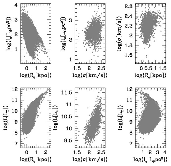
Figure 1.
The different projections of the virial plane. The panels including only photometric variables contain a much large number of ETGs with respect to those where the spectroscopic variable is involved.
- The scatter of the galaxy distribution is very different in every projection of the FP;
- There is a marked curvature in several observed distributions;
- Some regions in the diagrams are empty of galaxies, suggesting the possible existence of a ZoE;
- Although the samples used have different sizes, there is ample evidence (even coming from the literature) that the observed distributions have quite different scatters when the selection bias is taken into account (see Section 4).
It should be remarked that the construction of depends on L and , the luminosity, in turn, on the stellar mass and, finally, on and . Therefore, the large dispersion in each group can be ascribed to the large range of spanned by objects of a given mass.
The various planes of Figure 1 strongly hint that suitable relations among the three coordinates ought to exist. The most remarkable fact to note is the profound difference between the vs. and the L vs. relationships: the first is very dispersed, while the second is narrow. In other words, the tightness of the L vs. relation is largely due to the fact that the effect of varying from object to object is masked in the product ; equivalently, two objects with the same L may have different and (intrinsic degeneracy).
The aim of this work is to analyze these two diagrams: the and planes. These diagrams give us the opportunity to clarify the different roles played by luminosity in such correlations. Since both diagrams are projections of the same physical plane, the question arises whether it is possible to reproduce the galaxy distribution in one space starting from the other and vice versa. We will see that this is the case under some assumptions. If we rewrite Equation (1) as:
encrypting in the mean properties of the stellar population and its structural and kinematical properties, one can derive a theoretical expression for the FJ relation in a way similar to that used for the FP.
When we compare the observed distribution with Equation (4), it is easy to note that the observed FJ relation (see Section 4) is only a bit different from the prediction of the VT2. As for the FP case, the most accepted explanation for such difference is that a smooth variation of , essentially linked to the variable mass-to-light ratio and the structural/dynamical non-homology of ETGs, determines a different trend in the observed slope (much closer to 3 than 2).
It should be stressed that the classical FJ relation represented by Equation (4) does not say anything about the particular evolutionary state of a galaxy, i.e., if the luminosity is still increasing because of active star formation and/or mass accumulation by mergers or decreasing because no star formation is taking place and the bulk of stars are becoming older and older, and/or the galaxy mass is decreasing by interactions with nearby objects. What Equation (4) states is only that luminosity can be used instead of mass in the VT once the mean properties of the stellar population and the structure/dynamics of the systems are hidden in the parameter .
As a matter of fact, the luminosity of an ETG can simultaneously be written as:
where observations prove that ∼ and shows an rms scatter of ∼0.4 in log units. Since the errors on the single parameters involved in this equation are very small compared to the intrinsic range spanned by the single variables, we are mathematically legitimated to write:
which implies that the distribution can be recovered from the FJ relation through a simple analytical simulation under some assumptions on the behavior of and . In log units, we have:
Indeed, once the mutual variations of and are taken into account, and some values for and are adopted, it is quite easy to obtain the observed range of variation of as a function of , which can be compared with the observed distribution in the plane.
It is important to note, however, that the luminosity of each galaxy enters in the above equations only as a proxy of the stellar mass without considering its physical intrinsic characteristics, i.e., neglecting the role of mass accretion, star formation and evolution of the stellar content, while taking only the mean mass-to-light ratio into account. As remarked by [50], when the total luminosity enters in a SR, it brings with it a “degeneracy” that, depending on the correlation under exam, may imply either the use of L as a proxy of M or as the tracer of a past merger and the star forming activity and even the natural evolution of the stellar content. They showed that the total luminosity can be written as:
where is the time average of the current star formation, the luminosity per unit mass of a single stellar population, the age of the galaxy and the mean stellar mass-to-light ratio. This means that Equation (5) can also be related with Equation (8) and, consequently, that:
This demonstrates that the parameter might contain several variables and could be connected with several evolutionary properties of ETGs. In this case, must be strongly different from galaxy to galaxy and not be confined in a small range as it appears in the plane.
The solution for this problem could come from the hypothesis made by [50], who wrote the connection between total luminosity and stellar velocity dispersion in a conceptually different way from the FJ relation:
where and are now parameters strictly linked to the star mass assembly and the star formation activity (they can vary considerably from galaxy to galaxy). In Equation (10), the variables are not L and (that are observable quantities) but and , which are linked to the temporal variation of luminosity and velocity dispersion as the evolution proceeds. If this is true, Equation (7) can be also written in the form:
In the following, we will show that Equation (11) is able to reproduce the plane much better than Equation (7).
Before proceeding further, let us make some general considerations about our Equation (10) in light of recent understandings about the evolutionary histories of ETGs. Nowadays, it is clear that a single SSP or burst of star formation is not enough to explain their evolution. The mass-assembly history of ETGs is more complex and changing from galaxy to galaxy, modulated by their final mass (a proxy of their evolution), the dynamical stage (slow or fast rotators), the environment (central or satellite galaxies, isolated object or members or bigger complexes), etc. (see [57,58,59,60,61,62,63] for instance). Therefore, Equation (10) is a very simplified approximation of a more complex reality, in which ETGs present a wide range of possible star formation histories. Most likely both and are more complex functions than what it is assumed here. However, the parameterization expressed by Equation (10) will turn out to be fully adequate for our purposes.
The aim of this study is neither to address the question whether two families of ETGs with different formation and evolutionary history ought to be invoked to explain the distributions in the and planes (the so-called dichotomy) nor to rule out the FJ relation, which is the correct link between mass and stellar velocity dispersion. Rather, we aim to convincingly show that the classical FJ law is not able to create the link between the and planes. This link can only be established if we accept that Equation (10) is the right form to express the connection between total luminosity and stellar velocity dispersion. In this framework, the classical FJ relation becomes only the average relation produced by the new relation. We will see from the simulations that each galaxy follows its own evolutionary path.
A consequence of this is that the same explanation invoked by [50] for the tilt of the FP works for the tilt of the FJ relation. The assembly of points in the plane is the result of two different actions: from one side, the mass of a galaxy always constrains the range in luminosity and the values of , keeping the scatter around the FJ relation small (galaxies are always close to the virial equilibrium); on the other side, the luminosity of a galaxy depends on the history of mass accretion and star formation, probably keeping memory of the velocity dispersion of the gas clouds that formed its stars. In other words, mass and luminosity are two different physical quantities that do not follow the same evolutionary path exactly. As a matter of fact, even the pure luminosity evolution of stars progressively move mass and luminosity on different roads; the first remaining approximately constant and the second progressively decreasing. The key point is therefore to understand why luminosity, that is a non-linear variable linked to star formation and merging, is a good tracer of mass.
4. The Ie-Re Plane with the Standard FJ
In this section, we present the plane and the FJ relation that we obtain using the WINGS data. The distribution of galaxies in the plane for more than 30,000 ETGs is shown in Figure 2. First of all, we recognize the good similarity with the relation obtained by [4] (their Figure 4). The two families of ‘ordinary’ and ‘bright’ ETGs are well visible. In log units, the error bars affecting each point have a length of about 0.3 dex and turn out to be small compared to the large ranges of values spanned by and . Therefore, the error bars are not displayed in the plane of Figure 2.
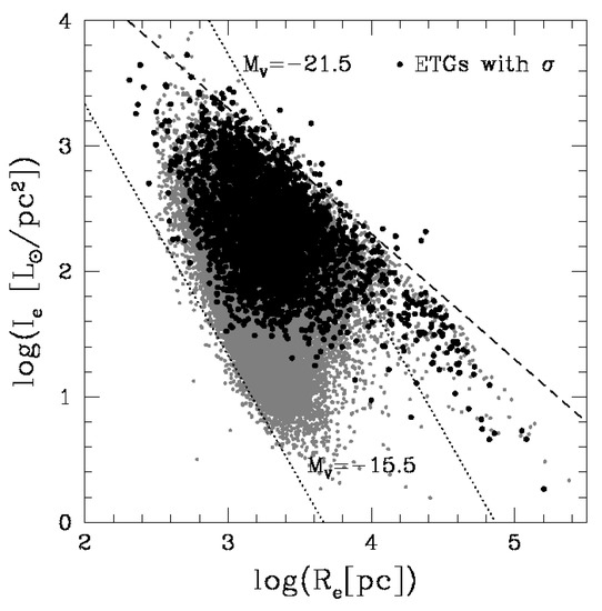
Figure 2.
Distribution of galaxies in the plane. The gray dots mark the WINGS ETGs. The black dots are the ETGs with available velocity dispersion. The dashed line marks the ZoE, i.e., the line with slope that is predicted for virialized objects. The dotted lines mark the locus of constant luminosity for and , respectively.
The features of interest in such a distribution are:
- The tail at large effective radii () for bright galaxies ();
- The cloud of ‘ordinary’ galaxies with maximum radii of 4;
- The sharp boundary due to the ZoE, i.e., the region avoided by galaxies of any type;
- The lower limit in magnitude at ∼, providing the maximum performance of the WINGS survey in detecting faint objects.
An obvious point of concern is whether the distribution of Figure 2 is affected by some systematic bias that could alter the observed shape. Chief among others is a luminosity selection. To highlight the issue, we plot the line of constant luminosity for (above which bright galaxies occur) and the line at that gives the magnitude limit of the WINGS survey. The slope of these lines is . This means that the distribution in the plane is necessarily different for galaxies of different luminosity. The brightest galaxies fall in the region at the right of the upper dotted line (the bright tail owes its name to this fact). This also implies that there is no magnitude bias in this plane. The only bias is that faint galaxies with are not present in the sample because they fall below the detection limit of the WINGS survey. The magnitude effect has no effect at all.
Finally, we want to highlight that the distribution of the ETGs with available velocity dispersion is almost identical to that of the photometric sample. This means that there is no bias working against the connection of the two planes. As a matter of fact, the plane shows a large distribution of points, while the plane does not, and this does not depend on the adopted samples.
We now present the FJ relation based on the WINGS data in Figure 3. In the upper panel, we display the plane so that the lower limits of the photometric and spectroscopic databases (close to ) can be compared. In the bottom panel, we show the same but in the plane. In both panels, the WINGs data are displayed only for galaxies with errors in both coordinates lower that 20%. The galaxies fainter are indicated by red dots and those brighter than by black dots. Finally, for the sake of comparison, we also plot the Illustris models for redshift (yellow dots).
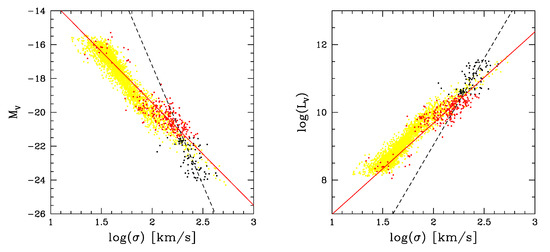
Figure 3.
(Lest Panel): The FJ relation in the vs. plane for the WINGS galaxies (black and red dots) and the Illustris simulation (yellow dots). The red dots and the solid red line mark the data and the fit for faint objects ( mag) with errors lower than 20%, while the black dots and the dashed line are the same but for bright galaxies ( mag). (Right Panel): the same as in the left panel but in the plane.
The observational data have approximately 1800 measurements of for ETGs (∼350 of which with very small errors), while the Illustris database contains instead ∼2400 objects. However, both samples span the same wide magnitude range going from to , although real data and theoretical models show different richness in different part of the relationship. This is simply due to observational (WINGS) and computational reasons (Illustris). At the low luminosity side, WINGS suffers a deficit of low luminosity (mass) galaxies with respect to the low mass ones for technical reasons, whereas, at the high luminosity interval, the Illustris database shows an obvious deficiency of high mass galaxies with respect to the low mass ones. All this is less of a problem in our study because what matters here is to check whether the theoretical and observational FJ relations have the same slope all over the range spanned by the data. As far as we can see, this seems to be the case with the possible exception of the brightest ETGs. Therefore, the classical Faber–Jackson relation [31], i.e., the log relation observed between total luminosity and central velocity dispersion, seems to be confirmed. Note the possible change of slope for the bright galaxies at ∼. The orthogonal fit marked by the black solid line, obtained with the SLOPES software [64] for the ETGs fainter than , gives:
For the galaxies brighter than , the orthogonal fit is:
In units, the slope of the FJ relation is ∼ for the faint ETGs and ∼ for the bright ETGs, while the scatter is always ∼. We, therefore, confirm the result of [32]. A summary of the fit parameters of the FJ relation for the ETGs of our sample are given in Table 1.

Table 1.
Fit of the Faber–Jackson relation for the WINGS and Omega-WINGS data in the and planes. The luminosity is in solar units and the velocity dispersion in km/s.
Despite the fact that the and relations cannot be built with the same galaxies because of the different sources of data, the ones we have presented are fully adequate as far as our aims are concerned, i.e., (i) to highlight the bi-modal distribution of the data in the relation and prove the curved behavior of the classical FJ relation that are seen to occur at the same luminosity in both diagrams (); (ii) to show that the distribution in the plane (Figure 2) is much broader and curved than that of the plane (Figure 3); and (iii) to call attention to the fact that it is not possible to pass from the FJ to the without using other information. In other words, as already pointed out above in Equation (5), we will demonstrate here that the classical FJ relation (luminosity steadily increasing with the velocity dispersion) of ETGs (Figure 3), in which and are confined in a small range, is not consistent with the distribution of the same objects observed in Figure 2.
Before proceeding further, we point out what follows: starting from the hypothesis that both the and planes originate from the FP (although in different ways), one could be led to believe that the different distributions of ETGs in the two planes is due to projection effects and/or selection effects affecting the different samples of ETGs in usage (those in Figure 3 are a subset of those in Figure 2 and therefore unable to account for the spread seen in the plane). This conclusion is not acceptable because the plane is not an orthogonal projection of the space but a contraction of the 3D FP to a 2D space ( and are contracted to L), so in this comparison, there is a missing variable. The mathematical simulation will demonstrate that the two distributions do not differ for selection or projection effects but because the hypothesis of keeping and almost constant does not work.
Going back to the FJ relation obtained with our data, we note that the slope ranges from 2.7 to 5.2 according to the luminosity (magnitude) interval covered by the data sample in usage (in the original FJ, the slope was ) and the zero-point also changes from 4.46 to passing from faint to bright objects (see the entries of Table 1).
For what concerns the quite large scatter of the FJ relation obtained here, we guess that it could be due to the presence of a large fraction of disky ellipticals that are known to be dominated by ordered stellar orbits in our sample, e.g., [65]. This is a well-known problem that has required the redefinition of the velocity dispersion as [66,67]. The discovery of these fast rotators among ETGs was a core result of the SAURON and Atlas3D surveys (see [68] for a detailed review of the topic). Taking this into account would lead to an FJ relation that is narrower than the classical one (about 0.05 dex thickness instead of about 0.1 of the standard case). To evaluate the maximum effect of on the plane, we suppose that . This implies a ratio and, keeping constant the mass and luminosity of a galaxy, a ratio . In the plane, an ordinary, low-luminosity galaxy (in which ) would be displaced by a factor of 0.6 in and 0.3 in . Therefore, the bulk of galaxies would still exhibit a broad distribution, leaving the correspondence between and unchanged.
We now start to explore Equation (7) to obtain the plane. Since and are each are correlated by the VT via the mass, we decided to use the dependence of on Re (, see below) and to express as a function of only. It is important to keep in mind here that, at each luminosity, only a small spread of possible is permitted by the FJ. The function can be derived from the WINGS database and is shown in Figure 4. As expected for each value of , there is a large dispersion of and vice versa at variance with the FJ. To cope with this, we try two kinds of fits of the relation with the SLOPES software [64]: the bi-linear least square fit (shortly bisector) indicated by the blue line and the standard least square fit (shortly best fit) shown by the magenta line in Figure 4.
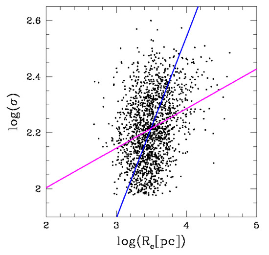
The bisector fit gives:
with an rms scatter of 0.11 and a correlation coefficient of 0.3.
The standard least square fit gives:
The resulting planes are shown in Figure 5, which displays again the data for the real galaxies with superposed the expected values of obtained from Equation (7) when we vary in the observed interval of measured values and we assume a given relation.
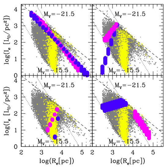
Figure 5.
Four different simulations trying to reproduce the plane from Equation (7). In all panels, the gray dots are the WINGS data and the yellow dots the Illustris data. (Upper Left Panel): the magenta dots are obtained assuming: , and . The blue dots are obtained assuming: , and . (Upper Right Panel): the magenta dots are obtained assuming: , and . The blue dots are obtained assuming: , and . (Lower Left Panel): the magenta dots are obtained assuming: , and . The blue dots are obtained assuming: , and . (Lower Right Panel): the magenta dots are obtained assuming: , , and . The blue dots are obtained assuming: , , and . The simulated galaxies falling into the ZoE region have not been plotted.
Note that the spread in the values of at each comes from the small scatter around observed in the relation. It is evident that the distribution in the plane depends on this relation and on the relation. The slope of the simulated distribution depends critically on the slope of the relation, whereas the scatter in the distribution (length of the thick bars) depends on the permitted variation of .
The upper left panel shows the case in which Equation (15) is adopted, can vary from 2.1 to 3.45, and may change from 5.65 to 2.65 with a scatter ∼. It is clear that, in this case, the ordinary family of ETGs is not reproduced. The upper right panel uses Equation (14) instead and the same values for and . Note the different slope of the simulated data and the small coverage of the plane. In the lower left panel, we use a steeper relation and a larger interval of values for . Again, only a small part of the plane is reproduced. Finally, in the lower right panel, we adopt two different functions obtained by putting Equations (14) and (15) together with the measured mass–radius relations for bright and faint ETGs derived by [56]. Again, despite the variations of and , only part of the plane is covered by the simulated data.
The most relevant fact to note in Figure 5 is that, even though the values of might vary significantly at any given , the small spread of around the values expected from the FJ of low and high luminosity ETGs does not permit covering the whole area observed in the space. However, if we artificially increase the scatter on , the becomes progressively filled by the blue and magenta simulations. We conclude that the standard FJ relation (either linear or curved) is incompatible with the observed distribution in the plane.
Why is this possible? What factor enters into the relation that is not present in the relation? According to D’Onofrio et al. [50], the problem resides in the FJ relation itself.
5. Digging Deeper into the FJ Relation
The FJ relation is, by construction, a fit of the observational data for a sample of ETGs, which simply mirrors the relation between mass and velocity dispersion, i.e., is a modified version of the VT, written using L instead of M (the total luminosity of a galaxy is primarily driven by the total mass). However, when applied to individual galaxies, the FJ relations loses a great part of its physical meaning because other parameters are also governing the luminosity of a galaxy, including the age of its stellar content together with the presence or absence of star formation activity. In other words, the true relation between L and might have a different origin and intrinsic complexity with respect to the simple VT.
The fact that the FJ relation is a translation of the VT is suggested by the value of its exponent , and it can be shown with simple arguments. The exponent of modern FJs falls in the range of 2.7 to 4 and even 5. Why? The luminosity of a galaxy is due to its stellar content, which, in turn, is composed by a manifold of single stellar populations (SSPs), each of which weighed by the star formation rate at the time of its generation. The mass-to-light ratio of old SSPs (the majority in ETGs) is nearly constant so that the total luminosity can be expressed as , where is the mass of the mean SSP and the stellar mass of the galaxy. The velocity dispersion of the stars is (the virial theorem). The radius is related to the mass by a relation of type , where observational data (see, e.g., [69,70]) and theory for the dissipationless collapse [71], leading to 0.5–0.6. This means that or, vice versa, that . Therefore, the exponent can easily be as high as 4 to 5 for ETGs. Therefore, the value for along the FJ can be easily recovered. For the sake of completeness, we recall that for CD galaxies, the value of is highly uncertain. According to Naab et al. [72], if a galaxy increases its mass by minor mergers, the radius should increase with the law , which implies that . Does it imply that the FJ relation can bend over at the highest luminosities, masses? The problem is still open. Fortunately, since our sample is nearly CD-free, we can leave the subject aside.
Looking for a more fundamental relation between luminosity and velocity dispersion of ETGs, which we suspect can be hidden in the classical FJ, in the absence of any other information, we make the ansatz of [50] that for each galaxy, the relationship keeps the formal dependence of the FJ relation but with exponent and proportionality factors that can vary from galaxy to galaxy. However, the collective behavior of any sample of ETGs should also obey the classical FJ, as clearly indicated by the observational data. In other words, we are looking for additional parameters that are missing in the classical FJ and not rejecting the FJ relationship.
In the law proposed by [5], the proportionality factor must depend on the star formation and mass assembling history of each galaxy, and the exponent must mirror the peculiar motion of each object in the plane across the cosmic epochs due to mergers and star formation events. Nevertheless, these two variables must be intimately connected to each other in order to keep the scatter of the observed classical relation small. This is an important constraint to keep in mind.
In the following, we intend to explore the consequences of our assumption, i.e., to look at the distribution of galaxies in the plane engendered by the law. In other words, we want to study the relation:
The main problem in this relation is that we do not know the present values of and for each galaxy. These values cannot be measured in a real galaxy without knowing its past history of mass accretion by mergers (or mass stripping by interaction) and star formation by different causes, both internal and external. The past values of L, , and for a galaxy are unknown. To cope with this, we resort to the Illustris simulations. With the aid of the Illustris model, we can, in fact, demonstrate that and are parameters subject to variations from object to object and across the cosmic epochs. In particular, the slope turns out to span a big range from large negative to large positive values. This analysis has already been made by [5] from whom we take the most salient results.
Here, we derive the possible value of by considering the variation in luminosity and central velocity dispersion of the same object between the different cosmic epochs (redshifts). All the data required by this analysis are available in the Illustris database. By construction, yields the displacement of a galaxy in the plane between two cosmic epochs. In Figure 6, we show the histogram of the values of obtained considering the two epochs at redshift and . We can see clearly that the values of are both positive and negative. The distribution of peaks in the interval 0 to 5 with wings at both sides up to 10 and −10. However, in the negative interval, the second peak occurs from zero to . This means that there are two numerous subgroups of galaxies whose luminosity either increases or decreases with . Furthermore, indicating the distribution of for the galaxies with with a black solid line and those with with a red thin line, we note that the big galaxies have preferentially negative values of ; this means that their luminosity decreased during the time interval from to . They are likely objects in which the star formation is either decreasing or has ceased and the bulk of stars are becoming less and less luminous at an increasing age.
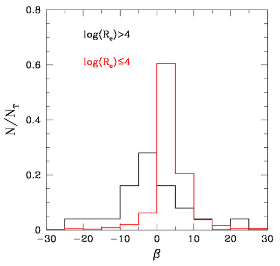
Figure 6.
Histogram of the values of derived from the Illustris simulation. The black (red) histogram is conducted for objects that have (), respectively.
Once is known, we must determine . We noted that using all pairs of progenitors-descendants (for which L and are known) of the Illustris samples for two near redshifts, a tight correlation between and can be derived. This is shown in Figure 7 for the particular case of and . The fit gives:
with an rms ∼5 and a correlation coefficient c.c. = .
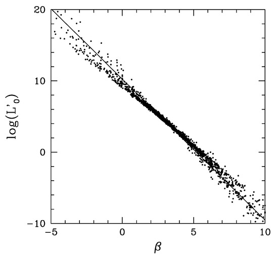
Figure 7.
The relation between and derived from the Illustris simulation. We plotted only the central interval with the most frequent values of .
The same procedure can be used for all the different epochs (redshifts) available in the Illustris database. Table 2 summarizes the slopes (), intercepts (), rms scatters and correlation coefficients for the relations between and obtained considering all redshift intervals to disposal. This correlation is rather strong and may easily account for the tightness and small scatter of the relation.
Table 2.
Slopes, intercepts, rms scatter and correlation coefficient (c.c). of the relations between and extracted from the Illustris galaxy models.
We can see in the Table that both the slope and intercept of the relationship smoothly vary with the cosmic time. The reason for this deserves future careful investigations. We suspect that it could be related to the variation of the mean star formation and merging rates of the galaxies with redshift (see, e.g., [73]).
Thanks to this result, we can explore the effects of varying and in Equation (17). By inserting Equation (17) and Equation (14) or (15) into Equation (16), we can see what happens to when we vary the effective radius in the range of the observational values. The technique we use is the Monte-Carlo method applied to . Once is known, we derive and to obtain and L and, finally, . Care is paid to vary each quantity within the permitted range of existence.
Figure 8 shows that when the relation is inserted into Equation (5), the plane is well reproduced, i.e., the real and artificial distributions almost overlap exactly, well beyond the natural uncertainty caused by the small size of the errors affecting the quantities in usage. This agreement leads us to claim that this is the correct solution for the mutual inconsistency between the distribution and the classical FJ relation.
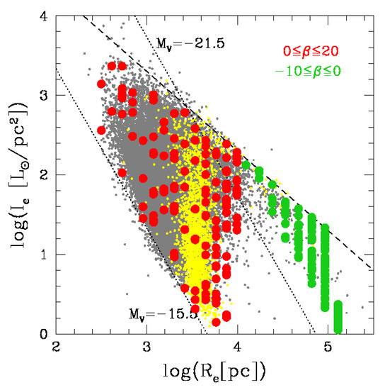
Figure 8.
The plane of Figure 2 with the data of the Illustris simulation in yellow. Red and green dots mark the artificial data obtained from Equation (16) when different values of and are considered. The artificial data above the ZoE have not been plotted as well as those below the limiting surface brightness of the observational data.
However, plotting the results for the distribution in Figure 8, we drop all cases that would fall in the ZoE region. Furthermore, we do not plot the points that fall below the lower limit in surface brightness of the WINGS survey. In conclusion, we can note the following:
- (i)
- The data with negative values of do fill preferentially the region of ‘bright’ galaxies;
- (ii)
- The data with positive values of are instead preferentially in the region of the ‘ordinary’ galaxies;
- (iii)
- The distribution of galaxies in this space critically depends on: (a) the assumed relation between and ; (b) the values adopted for the zero-point and slope of the relation.
- (iv)
- The density of simulated galaxies plotted on the figure depends on the adopted maximum width of interval spanned by , either positive or negative.
In addition, we note that:
- The distribution is not in contrast with the FJ relation, if the distribution for each individual galaxy is used;
- The negative values of are preferentially found in objects that are today in virial equilibrium and in a passive state of evolution, i.e., objects whose luminosity is now decreasing at nearly constant ;
- The shape of the distribution of galaxies in the plane depends only on their evolution in the plane. Both L and depend on the merging/stripping and star formation history experienced by each galaxy. When all this is over, the luminosity of the stellar content can only decrease by the natural dimming of the light emitted by the stars as time goes on.
An illustrative way for understanding the role of the parameters affecting the plane is shown in Figure 9. The figure shows four different cases in which we produce quite different distributions using Equation (16). The top panels show the effect of changing the relation of the galaxies, while the bottom panels show that for varying the values of and . Note that keeping and fixed and varying only as a function of , one obtains two distributions that do not fill the region of the ‘ordinary’ galaxies (upper panels). On the other hand, keeping the relation fixed, one can produce a distribution that is much more similar to that observed. The interval of permitted s is also important for determining the degree of filling of the plane (lower panels). At variance with the previous figures, we keep the galaxies falling in the ZoE here. Clearly, this mathematical exercise produces objects that do not exist in nature. This means that the distribution we observe in the plane is the result of a complex balance between the relation of each galaxy and the parameters and that define its evolution.
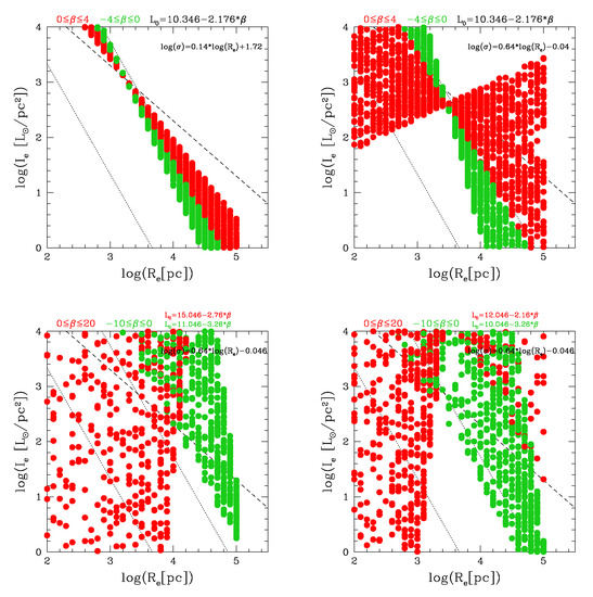
Figure 9.
Four different examples of the use of Equation (16) for reproducing the plane. In the top panels, the parameters and are fixed and the relation is changed. In the bottom panels, we make the opposite. The red and green dots mark the data with and , respectively. The dashed line is the ZoE, and the dotted lines are the curves of the constant at and .
To strengthen the idea that the relation is the one at work in individual galaxies, we perform in addition two experiments with the Monte-Carlo method.
First experiment. The procedure is as follows: (i) we select an array of values in the range typical of ETGs, i.e., ( in pc), and steps (16 values in total); (ii) to each , we associate a velocity dispersion according to Equation (14); (iii) given , we randomly choose the exponent in the interval , and with the aid of relation Equation (17), we determine ; finally, (iv) we derive the luminosity L from relation . The sequence from (ii) to (iv) is repeated 50 times. As a result of this, for each value of , we obtain an array of luminosities L. Each point has a different value of that can be either positive (red) or negative (green). Once L and are known, we derive . The total number of cases is about 800 so that the statistics are significant. The results are plotted in the plane of Figure 10 (left panel). In the same panel, we also display the data of our observational sample (the small gray dots). They show the classical FJ relation for the WINGS data. In the same plane, we also highlight the group of simulations that crowd the same area populated by the observational data (the red/green squares with a black contour enclosed by the black broken solid line). This same group is also plotted in the right panel of Figure 10 that displays the plane. The gray squares are the ETGs and the yellow dots the Illustris galaxies used for comparison. It is soon evident that with either positive or negative are equally legitimate in the plane and, vice versa, that the classical FJ relation is compatible with the idea that individual galaxies may, in reality, follow a dependence with both positive and negative. Simple considerations suggest that ought to be positive during the building up of the stellar content by the star formation triggered by internal (gas collapse) and external causes (mergers, interactions, shocks, etc.) and negative when this initial phase is over and the bulk of stars becomes older and fainter. In this simple experiment, cases are found that do not correspond to real ETGs (see the left panel). This is simply the consequence of the unconstrained Monte-Carlo procedure that does not include any of the physical processes taking place during the complex evolutionary history of a galaxy. For instance, we have not constrained the simulation by imposing a mass–radius relation that contrarily is present in the observational data3. Since the three relations are very similar, we only quote the one by [74] that is based on the richest sample (about 60,000 objects). This mass–radius relationship is:
where and are in solar units and kpc, respectively, the and the correlation coefficient c.c. . The maximum thickness of the relation is . What matters here is that within the area enclosed by the solid line in the left panel of Figure 10, which closely mimics the observational relation, both types of models are possible (red and green). Looking at the right panel of the same figure, the sequence of bright galaxies also contains red models (positive ) and green models (negative ). Finally, we note that both models are compatible with the observational plane.
Figure 10.
(Left Panel): The classical plane with the simulations in which each galaxy follows its own relation. The red dots have , and the green dots have . The black squares are the data selected as belonging to the FJ relation. (Right Panel): the plane with the same data selected in the left panel.
There is another interesting property to note. In Figure 11, we show the histogram of the values for the whole simulation (the black solid line) and for the models enclosed by the solid broken line in the right panel of Figure 10 (the red solid line). The initial uniform distribution of random numbers is now turned into a bi-modal one where a first peak is centered at and a second at .
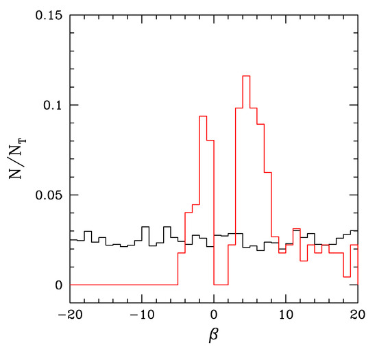
Figure 11.
Histogram of the values in the classical relation for model galaxies each of which obeys the relation. The black line is the histogram for the random assignment of to each model galaxy, while the red line is the resulting distribution of s in the group of models corresponding to the classical FJ distribution.
Second experiment. We have already argued that the galaxies obeying the classical FJ cannot reproduce the observed distribution in the plane with the current relation. The question can be raised whether galaxies that are nicely distributed in the plane and individually obeying the relation can reproduce the FJ relation. To this aim, we start from the plane of Figure 2, using the same WINGS objects of the known L, , and , to which the FJ relation of Figure 3 is associated. For these galaxies, we keep all parameters fixed, but suppose that the real correlation between L and is not but . Given L and , we suppose that can randomly vary between and 20, and for each value of , we derive the factor from Equation . As expected, we find that (i) all the values of and obey a relation very similar to that shown in Figure 7 but with minor differences, ; the values of show a bi-modal distribution with two peaks: one at and the other at (see the left panel of Figure 12). Then, we calculate the expected luminosity for values of in the interval 1.4 to 3 (i.e., covering the whole interval spanned by the observational data) in steps of 0.1 and all possible values of in the interval of to 20 in steps of 1. The above relation relation yields the value of to be used. The results are plotted in the right panel of Figure 12; the red triangles are for and the black squares for . These arrays of points represent all possible values of luminosity for each combination of and . In the same figure, we also plot the observational proposed for bright (massive) ETGs indicated by the central blue solid line with dots, together with two parallel lines of the same color showing the associated dispersion, and do the same for the less luminous (less massive) ETGs indicated by the green dashed lines. These relations are those of Table 1. An intersection occurs at . In general, the observational relations run in the quadrants for and through values of compatible with the observational determination of . However, there are regions in which both positive and negative values of are possible, i.e., in the interval . In this case, together with galaxies increasing the luminosity there are also others doing the opposite.
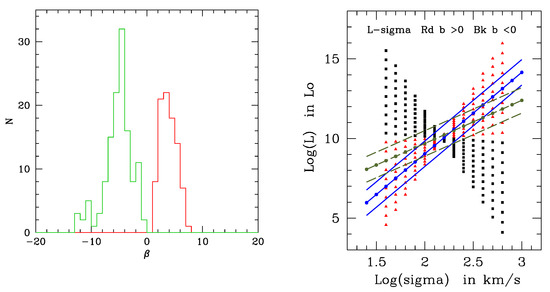
Figure 12.
(Left Panel): The histogram of the parameter of the relation applied to the galaxies used to build the plane. Two peaks are present, one in the interval and the other in the interval . (Right Panel): the classical relation expected for the same galaxies at varying parameter s. The velocity dispersion (, in km/s) goes from 1.2 to 3.2 in steps of 0.1. For each value of , we derive the specific luminosity from the relation previously derived from the simulations in the left panel. With the aid of the relation we obtain the luminosity. The red triangles are for , while the black squares are for . Finally, we plot two observational , i.e., for ETGs fainter than (green dashed lines) and those brighter than (solid blue lines). For each case, there are three lines: the central one is the mean relation, while the two wing lines yield an idea of observational spread around it. The comparison shows that while many objects are compatible with , there are others, fewer in number, that are compatible with . In any case, the mean value of (equivalent to of the classical interpretation of the relation) is positive.
Finally, we have also determined the mean slope of the two sub-populations weighed on the occurrence number per interval of : they are and . The slope of the final will depend on the percentages of the two populations with respect to the total.
In Figure 13, we show the predicted by this simulation together with the observational data. The green dots show the galaxies whose individual has negative . They are a small fraction of the total so that the mean slope of the whole sample with remains with positive and in the range 4 to 5, while the remaining population also has positive but with lower values falling in the range 1 to 3. Finally, we would like to point out that the galaxies with are those along the tail towards low surface brightness in Figure 2.
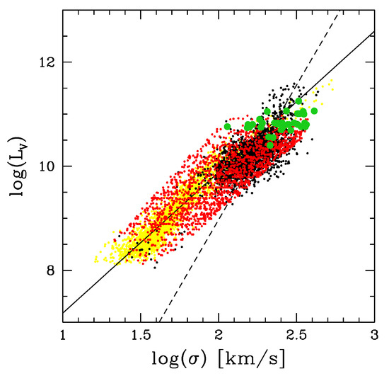
Figure 13.
The classical plane with the simulations in which each galaxy follows its own relation. The red dots are , and the green dots are . The black dots are the data of the classical FJ relation. The green dots are confined in the region of bright ETGs. In our view of the problem, this means that the luminosity is decreasing; in other words, no star formation or mass building is taking place in these galaxies.
In conclusion, these experiments lend strong support to the hypothesis that, masked by the classical relation, there is another relation driving the behavior of each individual galaxy. For the latter, we have assumed the same analytical dependence of the but with the proportionality factor and exponent that vary from galaxy to galaxy. This hypothesis is also supported by the Illustris models of galaxy formation in a hierarchical scheme. Thanks to this hypothesis, the incompatibility between the plane and the standard can be ruled out.
6. Discussion
We have demonstrated above that the and distributions are only mutually compatible if we accept the idea that luminosity and velocity dispersion of each individual galaxy are related by the law, where and vary from galaxy to galaxy and over the course of time. The relation hides the complex interplay between the baryonic and dark matter components of a galaxy and the mass accretion and star formation history experienced by each galaxy. Contrary to the classical , the new relation does not originate from the VT but leads to results that are compatible with it.
The idea behind this new perspective is that the total luminosity of galaxies is essentially the result of the mass assembly, star formation history and temporal evolution of the stellar populations inside. Therefore, the luminosity of a galaxy is expected to be a complex function of all these phenomena. It is worth recalling in this context that long ago, Brosche [75] questioned the simple, largely empirical, star formation law of Schmidt [76], based only on the gas density , and favored a scenario in which the star formation and the rate at which it occurs are functions of several parameters, among which we recall the gas density and the rotation velocity , where may vary from galaxy to galaxy. Stars born in large gas complexes have a characteristic velocity that depends on the physical condition of the galaxy during the star formation event (collapse, shock, merging, etc.). For this reason, the global star formation and galaxy luminosity (the chief fingerprints of stellar activity) ought to keep memory of the gas velocity. The work of Brosche [75] spurred D’Onofrio et al. [50] to introduce the new relation.
To lend support to this idea, we resort again to the Illustris simulations and look at the properties of galaxies at different epochs (redshifts). To this aim, we randomly select a small number of galaxies out of the sample at , for which we know the whole history through the cosmic epochs for the set of redshfits provided by Illustris, i.e., we know the sequence of progenitors that, through a number of mergers, gave origin to the objects seen at . We limit this to the redshifts and . For this small sample of galaxies, we know how the basic quantities , , and L have changed with time. The results for three typical cases are shown in Figure 14, which displays the plane on the left, the plane on the top right and the plane on the bottom right. The color code is blue for models at , green for models at , red for models at and, finally, gray for the observational data at .
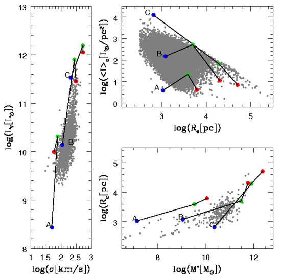
Figure 14.
(Left Panel): The FJ plane. The gray dots are the observational data from the WINGS database. The filled circles of different colors are the three ETGs of the Illustris database taken at different redshift epochs: (blue), (green) and (red). (Right Panels): the plane (upper plot) and the plane (lower plot). The gray dots are again the observational data present in the WINGS database. The samples have different sizes in each plot because the spectroscopic and photometric datasets have different richness.
In relation to our discussion, the models plotted on the plane are particularly enlightening. Let us compare the models to each other at a given redshift with the data at . The three blue circles, green circles and red circles separately draw sequences in which the luminosity grows with the velocity dispersion, i.e., follows the classical relation, the dispersion of which always remains rather small. The sequence of red circles is fully compatible with the present day data (gray dots). In other words, during the cosmic evolution in the hierarchical scheme, the FJ relation is in place, although with a slightly different slope at each redshift. The whole ranges spanned by L, and progressively shift to higher and higher values. This indirectly confirms that the FJ simply mirrors the relation. What is mostly relevant here anyhow is that all the three cases shown here present a decrease in luminosity at nearly constant passing from to (in one case, even decreases), the opposite occurs from to . In general, looking at many other cases not shown here for the sake of clarity, the path of a galaxy in the plane is a combination of different possible trends depending on the accretion history of mass. In brief, the general trend follows the relation, while individual galaxies follow the law.
The distribution of theoretical models in the plane is intriguing and needs some explanation. We start labeling the three groups of models “A, B, C”, as indicated in the panels of Figure 14. With our cosmological parameters, the present age of the universe is Gyr, while at the redshift epochs of the models, it is Gyr and Gyr. Taking ( Gyr) as an indicative redshift for the start of galaxy formation, the age of the model galaxies are Gyr, Gyr and Gyr, with . Along each sequence A, B, C, the radius and mass increase, as indicated in the top and bottom right panels of Figure 14, respectively. Having set the scene, we note that: (i) the most massive and oldest objects (red circles) of each sequence draw a curved line in the plane that nicely coincides with the border of the galaxy distribution in this plane. The other models overlap the data. (ii) As the mass and size of galaxies increase, they move progressively toward the limits imposed by the ZoE, i.e., the limit drawn by galaxies in virial equilibrium and passive evolutionary stage (see [5]). (iii) The tail in the plane corresponds to the tail of the plane (see the bottom right panel of Figure 14). (iv) As already said, the data refer to galaxies at , so the comparison of data with models for and requires that the ages of these latter are suitably rescaled. It is obvious that the age of models born at and seen at , e.g., , is fully equivalent to a model born at and observed now. This allows us to consider all the galaxies in the plane as spanning a wide range of ages from the last episode of star formation dominating the light (and luminosity and surface brightness in turn). Pre-existing stellar populations in each galaxy that were generated by the past merger and star forming activity would determine the stellar mass , radius , velocity dispersion and part of the light. In brief, the large scatter in the plane can be easily accounted for.
Coming back to the characteristics of the and planes, the first interesting feature of both diagrams is the existence of ‘tails’ in correspondence of the most massive systems. These tails are well reproduced by the Illustris models [5]. The plane has also been thoroughly investigated by [56]. The tails are formed by objects with a mass higher than and seem to appear starting from redshift . On the basis of the previous discussion, the formation of the bright family tails in the (and the planes) can be associated with the quenching of the star formation activity (both spontaneous and/or triggered by mergers).
The second relevant characteristic is the existence of two groups. In the plane, the ‘ordinary’ family, in which , and the ‘bright’ family with are well visible. This latter owes their large radii to the variation of the effective radius, possibly induced by minor merger events [5,72]. Such events likely change the whole structure of the galaxies and consequently modify the Sércic index n of the light profiles to values higher than 5. The mergers of stellar systems with no gas should engender systems with dimensions larger than usual for a given total mass because no dissipation of energy can take place with the generation of new stars (see also the discussion in [56] for more details). However, even ignoring the effect of minor mergers, could decrease by natural fading of the luminosity emitted by the stellar populations of a galaxy and the absence of any rejuvenation of the stellar content by the star formation. The inspection of current libraries of stellar populations, e.g., [77,78], shows that the magnitudes and scale linearly with , which means that the total luminosity can easily go down by a large factor past the last significant episode of star formation, thus causing a large decrease in even if remains nearly constant.
In this framework, it is also instructive to examine the following parameters extracted from the Illustris simulation: the stellar mass , the total luminosity L, the star formation rate (in per year) and the stellar velocity dispersion . The results are shown in the four panels of Figure 15. The color code indicates galaxies at different redshifts, namely (blue dots), (green dots) and (black dots). The upper left panel shows the plane. It is evident that at , many galaxies are decreasing their (the rain of dots toward low values of ). The process is also visible at , while it is absent at . The same trend is visible in the plane (the upper right panel). The brightest galaxies, in particular, are those where the is drastically decreasing. Notably, the plane (bottom left panel) shows how the mass-luminosity relation tends to bend with an increasing mass (the luminosity decreases because the decreases). The relation is steep at and much less steep at ; the scatter, however, is quite similar in all cases. Finally, the same trend is visible in the bottom right panel showing the vs. plane.
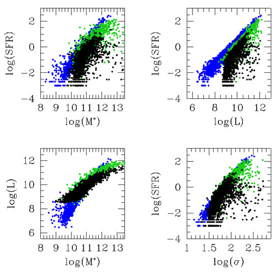
Figure 15.
(Upper Left Panel): the relation at three different redshifts: (blue dots), (green dots) and black dots. (Upper Right Panel): the relation. (Lower Left Panel): the relation. (Lower Right Panel): the relation. Stellar masses are in and are indicated by in the plot, in , luminosities in and velocity dispersions in km/s.
The evolution along the plane has been the subject of many studies using cosmological surveys, compilation of data and fossil records (see, for instance, [79,80] and references therein), while the evolution along this diagram of present-day ETGs was presented by Sánchez et al. [81]. Although the comparison of the Illustris results with those studies is beyond the aims of this study, the mutual agreement is fairly good, securing that the Illustris models can be safely used in our analysis.
The last test using the Illustris data, made to better understand the behavior of galaxies in the and planes, is a simple experiment conducted using the values of predicted by the simulation in correspondence to the changes of , , L and passing from one value of the redshift to another. We compare here the variations in and in luminosity predicted by the simulation between seven pairs of redshift intervals. Figure 16 shows the plane for all these redshift intervals using different colors in the left panel. The right panel shows the possible shifts of a galaxy in the left panel passing from one redshift to another. Each panel is made of four quadrants according to the combinations of positive and negative values of and . The left panel of Figure 16 shows that the galaxy transformations occurring at nearby epochs, marked by gray and brown dots, are preferentially located in the left quadrants of the plot, where and . On the other hand, those at a high redshift are preferentially observed where and . The right panel of Figure 16 schematically sketches the change in the properties of galaxies located in the different quadrants of this diagram. By construction, ); therefore: (i) Galaxies that have and are likely objects that have lost mass and are consequently less luminous, (but the direction of their motion in the plane is that with ). The only process that can give such result is the stripping of a significant amount of stars during galaxy encounters. (ii) Galaxies with and have decreased their luminosity at nearly constant mass, or their mass has moderately increased ()), but the luminosity decrease is very large. (iii) Galaxies where and are still merging with each other so that both the mass and the luminosity increase. (iv) Finally, galaxies with and are those probably rich of gas that have lost stellar mass () during a close encounter. In this case, shocks might induce a burst of star formation increasing the luminosity, but the total mass of the galaxies decreases.
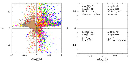
Figure 16.
(Left Panel): the plane. The epochs of different redshifts are marked by dots of different colors: the most remote one, starting at and going to (blue dots), is followed by that from to (green dots), that from to (magenta dots), that from to (yellow dots), that from to (red dots), that from to (gray dots) and that from to (brown dots). (Right Panel): a sketch of the same plane showing the variation of mass, luminosity and velocity dispersion associated to each position of a galaxy in this diagram. The left and right panels are, in turn, made of four quadrants according to the combinations of positive and negative values of and .
According to the values of and each galaxy has its peculiar motion in the plane. The galaxies belonging to the upper part of the diagram with do move along the relation, while those with move perpendicularly to this relation.
Figure 17 now shows the distribution of the for the galaxies belonging to the different quadrants of the left panel of Figure 16 at two values of the redshift: namely (upper panel) and (lower panel). We can see very clearly that the situation significantly changes passing from one redshift to another. At , most of the galaxies fall in the red and blue histograms, i.e., they are galaxies that have lost significant amount of mass and/or are now in a quenched state of star formation (). On the contrary, at , most of the galaxies fall in the green and black histograms, i.e., they are galaxies still undergoing a merger or have formed new stars soon after a close encounter where they have lost part of their mass.
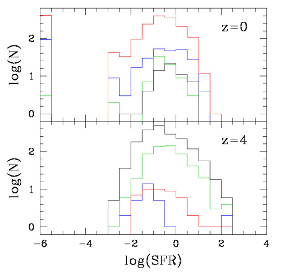
Figure 17.
(Upper Panel): histogram of the SFR at for the galaxies belonging to the four parts of the diagram. Blue lines mark galaxies with and ; green lines mark those with and ; red lines mark those with and ; black lines mark those with and . The galaxies that have have been assigned to the bin . (Lower Panel): the same histogram for the galaxies at .
Finally, we can address the question of the distribution of ETGs in the plane from the point of view of analytical models of galaxy formation and evolution. To this aim, we resort to the simple models developed by Chiosi [82], extended by Tantalo et al. [83] and recently used by Chiosi et al. [73] to study the cosmic star formation rate and by Sciarratta et al. [84] to investigate the galaxy color-magnitude diagram. In brief, a galaxy of total mass is made of baryonic (B) and dark matter (D), with mass and , respectively, and, at any time, satisfies the equation:
The baryonic mass is supposed to be originally in the form of gas to flow in at a suitable rate and, when physical conditions allow it, to transform into stars. With the same rate, dark matter also flows in, together with baryonic matter, to build up the total gravitational potential. A suitable prescription is adopted to describe their spatial distribution (see [83] for more details). Baryonic and dark matter are in proportions fixed by the adopted cosmological model of the Universe. This kind of galaxy model is named ‘infall model’, the essence of which resides in the gas accretion into the central region of the proto-galaxy at a suitable rate (driven by the timescale ) and in the gas consumption by a Schmidt-like law of star formation. The gas accretion and consumption coupled together give rise to a time dependence of the closely resembling the one resulting from the N-body simulations, e.g., [85,86,87,88]. At any time t, the baryonic mass is given by the sum:
where is the gaseous mass and the star mass. At the beginning, both the gas and the star mass in the proto-galaxy are zero . The rate of the baryonic mass (and gas in turn) accretion is driven by the accretion timescale according to
where is the accretion timescale and a constant with the dimensions of (Mass/Time) to be determined by imposing that, at the galaxy age , the total baryonic mass of the galaxy is reached:
Therefore, by integrating the accretion law, the time dependence of is:
The timescale is related to the collapse time and the average rate of gas cooling. Therefore, it is expected to depend on the mass of the system. The gas mass not only increases by infall but also decreases by star formation. The rate of star formation is modeled throughout the whole life of the galaxy with the [76] law:
where k regulates the dependency of on the gas content (classically, it can be linear or quadratic: we fix it as ), and is the efficiency parameter of the star formation process.
In the infall model, because of the interplay between gas accretion and consumption, the starts low, reaches a peak after a time approximately equal to and then declines. The functional form that could mimic this behavior is the time delayed exponentially declining law:
The Schmidt law in Equation (24) is therefore the link between gas accretion by infall and gas consumption by star formation.
As a whole, this kind of approach stands on a number of observational and theoretical arguments, among which we recall: (i) the parameters and can be related to morphology [89] and the presence of ongoing star formation activity inside observed galaxies [90]; (ii) the aforementioned quantities can be easily tuned in order to fit observational data, and complex phenomena that would affect the rate of gas cooling, such as active galactic nuclei (AGN), can also be empirically taken into account without going into detail (see, e.g., [73]). These galaxy models include many important physical phenomena, for instance, gas heating by supernova explosions (both type Ia and type II), stellar winds, gas cooling by radiative emission, galactic winds and the presence of dark matter in shaping the gravitational potential. See the study by Tantalo et al. [83] for all details on these topics. The list of the key model parameters used in this study is given in Table 3.
Table 3.
The key parameters of model galaxies: , and . Masses are in solar units and in Gyr.
A short comment is necessary about the efficiency of star formation , which has been assumed to be independent of the galaxy mass (morphological type) and thermo-dynamical condition of the gas. While this assumption is fully adequate to our present aims, it is not in line with the recent understanding of this parameter. Colombo et al. [91] showed that the depletion time associated with the efficiency depends on the morphology (and mass); the results were later confirmed by Sánchez et al. [92] and Sánchez et al. [93] using direct and indirect estimations of the molecular gas content in galaxies and the distribution of elements in galaxies.
Three series of models are calculated with the same input parameters:
- (i)
- In the first group, there is no constraint on the star formation activity, which never stops in the course of formation and evolution. Although reduced to minimal levels of activity, the star formation is also active at the present age. However, even minimal traces of star formation should be excluded for present ETGs. For this reason, we calculate a second group of models (see below) in which the is zero at the present time. The results indicate that, in practice, there is no effect on our analysis.
- (ii)
- In the second group soon after the activity peak (approximately soon after the age , when the bulk of stars is already in place), star formation is stopped. Consequently, at the present age, the light emitted by the galaxies is free from contamination by newly formed stars. This allows us to evaluate the effect on the luminosity and , in turn, by ongoing star-forming events. As already mentioned, we evaluate the decrease in luminosity in the range 1 to 2. We take the lowest value as a minimum estimate. At each time, we evaluate the radius of the stellar component by means of the mass–radius relation (MRR) proposed by Chiosi et al. [56]. The MRR of Chiosi et al. [56] is:where is in kpc and in . The variable is the ratio of dark to stellar mass and, in principle, can vary with the galaxy mass; here, we assume the typical mean value (see [56] for all details);
- (iii)
- In the third group, we examine the effect of the MRR. While massive galaxies (mass greater than about ) at the present time obey a sharp MRR, this is not the case of less massive galaxies whose and are apparently weakly correlated. They indeed crowd in a cloud on the MR-plane, although a weak correlation can be derived (see [56] for a thorough discussion of this problem). To this aim, we calculate a third group of models in which the MRR for less massive galaxies is taken from Woo et al. [94], which is much flatter (about a factor of two) than the one adopted for the more massive galaxies.4 Finally, the luminosity of the galaxy as a function of time is calculated with the population synthesis technique described in Bressan et al. [95] so that the detailed star formation history is taken into account.
The results are shown in Figure 18, where the blue lines are for the models with the standard MRR and no constraint on the , while the red lines are for those with interrupted . In the same figure, the green and magenta models are the same (green for active star formation and magenta for extinguished star formation) for those with the flatter MRR in the range of low mass objects. The dashed line is the ZoE.
Figure 18.
The plane of the analytical model galaxies with infall. The mass grows from left to right in steps of a factor of 10 from to . The infall time scale and specific efficiency of the star formation are listed in Table 3. The relation is from Chiosi et al. [56]. The blue lines are models with active star formation all over the evolutionary history. The red lines are models in which star formation is quenched off past the age . The green and magenta lines indicate the model with active (green) and quenched off (magenta) star formation, but in which the relation for galaxies with stellar mass in the interval to is that of dwarf galaxies of Woo et al. [94]. See the text for more details. The dashed line is the ZoE.
Looking at the first and second group (models with standard MRR and different SFR), it is worth recalling that a galaxy moves along this line from the top to the bottom at a decreasing speed because the variation in luminosity tends to slow down as the evolution proceeds. The present age is the last point of each line. The distribution of the final stage (present age) mimics the distribution of observational data in the plane. Large radii are reached by massive galaxies thanks to the adopted MR relation. Remarkably, all the final points of the blue lines fall either along or below the ZoE, and those of the red lines are well below this. The obvious implication is that the effect of star formation cannot be ignored when examining the properties of the plane. Passing now to the third group (models with shallower MRR for less massive galaxies), thanks to their larger radii at a given , they greatly shift toward lower and larger . Since from the observational point of view, galaxies in this mass range show radii in the range predicted by Chiosi et al. [56] and Woo et al. [94], the terminal stages of all models presented in Figure 17 encompass all reasonable situations that can be seen at the present time in this diagnostic plane. Furthermore, they provide an idea of the spread to be expected because of a spread in the epoch of galaxy formation (galaxies nowadays detected in different evolutionary stage), different histories and different histories of their dimensions caused by internal (galactic winds) external (mergers) events. They also strongly suggest that the most massive galaxies ceased their star formation histories back in the past. Moreover, these results are in perfect agreement with the observational data in Figure 2. Finally, it lends strong support to the notion that the ZoE is traced by galaxies in virial equilibrium and passive internal evolution.
From an observational perspective, the tails of bright galaxies in the and planes trace the border of the ZoE. When a galaxy reaches the passive state of its stellar content with no star formation activity, no important energy injections by supernova explosions and no significant mergers, it soon relaxes to virial equilibrium.
We name this ideal situation a state of ‘full virial’ condition. In this context, in the various diagnostic planes, such as the and also the so called kappa-space defined by [28,29], there is a special locus populated by galaxies in this ideal state: virialization and passiveness.
As demonstrated by [5], the intersection of the VT equation with the relation naturally explains the origin of the ZoE. Their Tab. 4 indeed shows that the slopes achieved in the and planes are converging to a limit of and 1, respectively, when becomes progressively more negative. Objects beyond this limit cannot exist, as the ZoE is acting as a physical barrier in the (and ) plane. When a ‘bright’ galaxy is in this state, is negative because the luminosity can only decrease. Consequently, the path followed in these diagrams by galaxies in this peculiar state of evolution cannot deviate from the limiting slope fixed by the intersection of the relation with the VT. Such condition preferentially occurs in massive galaxies because they rarely undergo major mergers and are scarcely affected by the minor ones. They are also passive objects since their stellar content indicates that star formation has ceased long time ago. Therefore, massive galaxies are the closest systems to the condition of ‘full virialization’. Consequently, their luminosity must decrease at a nearly constant (high negative values of ). For the objects of the ‘ordinary’ family, the full virial equilibrium is frequently disturbed by mergers with other objects of comparable mass, the removal of stars and gas by interactions with other galaxies and intense star formation activity either continuous or in sporadic episodes. Although virial equilibrium can be reached on dynamical time scales, in reality, these objects are often far from the ideal condition of full virialization and passiveness and therefore far from the ZoE. Consequently, their luminosity can both increase or decrease and so does their velocity dispersion, and their can be positive or negative and low or high.
From the above considerations, we can deduce the following conclusions:
- (i)
- The galaxies that move almost perpendicularly to the FJ relation in the plane are those with , i.e., they are either inactive in forming stars or experiencing a burst of star formation triggered by a close encounter with another galaxy during which they underwent significant mass loss;
- (ii)
- The galaxies while loosing or acquiring mass by close encounters and/or mergers move along the FJ relation. The deviations from the FJ distribution is always small, keeping the scatter observed at .
- (iii)
- The classical FJ relation must be understood as the mean behavior on the present day plane of the path followed by each galaxy with its own values of and . The slope and proportionality factor of the FJ should be given by the mean values of and of the sample under consideration, i.e., and . The problem is that the arrays of s and s are not known, unless one resorts to simulations, such as Illustris. Introducing the distribution has no practical advantage, but it clarifies that the information provided by the classical FJ is not enough to highlight the complexity of physical phenomena hidden in the and relations. It is mandatory to obtain a relationship between the luminosity of a galaxy and not only its stellar mass but also other properties, such as the radius (at least) and the past history of mass assembly and star formation, from general principles.
7. Conclusions
In conclusion, the present work has demonstrated that:
- The distribution observed in the plane originates from the relation, in particular, on the spectrum of values attained by and that each galaxy can experience during its evolution;
- The distribution does not depend on the definition of and (see the arguments by [16]) but only on the history of mass assembly, mass removal, star formation and evolution of the stellar content;
- All the scaling relations based on the effective radius can be interpreted as originating from the combination of the VT and the distribution.
- The law does not replace the FJ relation. They are two different things. The FJ relation mirrors the fundamental and obvious fact that the total light emitted by an assembly of stars is almost proportional to their total mass. In the FJ, the total light is the luminosity, and the total stellar mass is replaced by the velocity dispersion via the VT (some hints on the radius-mass relation is, however, required). Furthermore, the FJ relation is a 2D representation of the 3D space of the FP. Passing from 3D to a 2D space, some degeneracy among two of the three variables is introduced. The distribution intends to remove this degeneracy when going back from the plane to the plane. The task is achieved by looking at the evolutionary history of the quantities L, , and that is reconstructed with the aid of the library of hydrodynamical large-scale simulations of structure formations and evolution in the hierarchical scheme. In this context, each galaxy is characterized by its own and its history, represented by a different path in the plane, a path that varies with time.
- The FJ is a snapshot of the L- plane taken at the present time, and the relation is the average location of all the individual positions of galaxies, as seen at the present time. Thanks the relation and its time variation shown by the Illustris simulations, we can now go deeper into the physical causes generating the FJ relation and the plane.
- In our relation, the terms and resume the history of the mass assembly of galaxies. in particular must depend on the inverse ratio of the stellar populations (see Equation (9)). Luminosity can be expressed as the product of and . If ETGs follow a downsizing trend, then one expects their ratio to increase with the galaxy mass () with the brightest ETGs completing their mass assembly earlier than the lower-mass ETGs and showing the highest ratios (see [88] and references there in). If this is the case, then ordinary ETGs should, on average, be characterized by a lower mass and light-weighted stellar age than brighter ETGs. In other words, the exponent should follow an inverse relation with the light-weighted stellar age (negative s for bright ETGs that have experienced passive photometric evolution since redshift ). Our analysis already lends support to this view that could be better strengthened by detailed spectro-photometric evolutionary descriptions implemented in numerical NB-TSPH models of ETGs.
The last thing to comment on is the problem of the trend observed in the relations and (central surface brightness), which are both linear. Why do we not see any curvature in these relations? Our explanation is that all of them simply mirror the virial relation, which, in turn, has the mass as a driving parameter, i.e., they are not real relations involving the luminosity of galaxies and its history. The real driver of these relations is the mass of the galaxies instead of the luminosity, as is the case of the FJ relation. The luminosity affects the scaling relations when the half-luminosity radius and the effective surface intensity are taken into account as key parameters.
Concerning the relationship, it is likely that is a parameter that does not depend on the past history of a galaxy, made by mergers and star formation, but a local property strongly dependent on the total mass.
In conclusion, we can say that the law proposed by [50] and analyzed by [5] has now a solid empirical evidence because it can easily explain the distribution of real galaxies in the observed and planes (and others projections of the FP) but also a theoretical basis grounded on the numerical simulations. The law must therefore be considered the ‘true’ relation connecting luminosity and velocity dispersion. The parameters and of present-day galaxies encrypt the history of the mass assembly made by mergers and star formation and can likely be derived by combining two or more projections of the FP that turn out to depend on them (D’Onofrio et al. in prep.). Their presence, evolution and significance can be linked to theoretical studies on the star formation and merging activity, for example, by exploring the effects of a star formation depending not only on the gas density but also on the clouds’ velocities or by numerical simulations of merger events. These parameters can also be useful for characterizing the evolutionary status of a cluster of galaxies—their values being a proxy of the galaxy evolution (activity or quenching). This important subject is left to future studies. It is highly desirable that, in the near future, by deciphering the physical processes encoded in the parameters and , we may identify the possible ancestors of present day galaxies.
Author Contributions
Writing–review & editing, M.D. and C.C. All authors have read and agreed to the published version of the manuscript.
Funding
This research received no external funding.
Acknowledgments
We are deeply grateful to our referees for their comments that helped us to improve several points of the manuscript. C.C. thanks the Department of Physics and Astronomy of the Padua University for the hospitality and computing support.
Conflicts of Interest
The authors declare no conflict of interest.
Notes
| 1 | The formal definition of effective surface intensity is . For the sake of simplicity, we drop the notation of the mean value and write . In the whole paper, by the notation we mean the plane versus in suitable units. |
| 2 | This is again the well-known problem of the FP “tilt”. |
| 3 | See, for instance, the three relations for ETGs analyzed by [56] using the data by [29,74], and WINGS. |
| 4 | The MR relation for low mass galaxies (the dwarf galaxies) in the mass interval to of Woo et al. [94] is . See the paper for all details. |
References
- Dressler, A.; Lynden-Bell, D.; Burstein, D.; Davies, R.L.; Faber, S.M.; Terlevich, R.; Wegner, G. Spectroscopy and Photometry of Elliptical Galaxies. I. New Distance Estimator. Astrophys. J. 1987, 313, 42. [Google Scholar] [CrossRef]
- Djorgovski, S.; Davis, M. Fundamental Properties of Elliptical Galaxies. Astrophys. J. 1987, 313, 59. [Google Scholar] [CrossRef]
- Kormendy, J. Brightness distributions in compact and normal galaxies. II. Structure parameters of the spheroidal component. Astrophys. J. 1977, 218, 333–346. [Google Scholar] [CrossRef]
- Capaccioli, M.; Caon, N.; D’Onofrio, M. Families of galaxies in the mu.e-R.e plane. Mon. Not. RAS 1992, 259, 323–327. [Google Scholar] [CrossRef]
- D’Onofrio, M.; Chiosi, C.; Sciarratta, M.; Marziani, P. The parallelism between galaxy clusters and early-type galaxies. II. Clues on the origin of the scaling relations. Astron. Astrophys. 2020, 641, A94. [Google Scholar] [CrossRef]
- Capaccioli, M.; Caon, N.; D’Onofrio, M. The (log re,μe) Plane of Hot Stellar Systems. In Proceedings of the European Southern Observatory Conference and Workshop, Monterey, CA, USA, 25–29 October 1993; Volume 45, p. 43. [Google Scholar]
- Kormendy, J.; Fisher, D.B.; Cornell, M.E.; Bender, R. Structure and Formation of Elliptical and Spheroidal Galaxies. Astrophys. J. Suppl. Ser. 2009, 182, 216–309. [Google Scholar] [CrossRef]
- Kormendy, J.; Bender, R. A Revised Parallel-sequence Morphological Classification of Galaxies: Structure and Formation of S0 and Spheroidal Galaxies. Astrophys. J. Suppl. Ser. 2012, 198, 2. [Google Scholar] [CrossRef]
- Tolstoy, E.; Hill, V.; Tosi, M. Star-Formation Histories, Abundances, and Kinematics of Dwarf Galaxies in the Local Group. Annu. Rev. Astron. Astrophys. 2009, 47, 371–425. [Google Scholar] [CrossRef]
- Somerville, R.S.; Davé, R. Physical Models of Galaxy Formation in a Cosmological Framework. Annu. Rev. Astron. Astrophys. 2015, 53, 51–113. [Google Scholar] [CrossRef]
- Kormendy, J. Elliptical Galaxies and Bulges of Disc Galaxies: Summary of Progress and Outstanding Issues. In Galactic Bulges; Laurikainen, E., Peletier, R., Gadotti, D., Eds.; Springer: Basel, Switzerland, 2016; Volume 418, p. 431. [Google Scholar] [CrossRef]
- Caldwell, N. Structure and stellar content of dwarf elliptical galaxies. Astron. J. 1983, 88, 804–812. [Google Scholar] [CrossRef]
- Binggeli, B.; Sandage, A.; Tarenghi, M. Studies of the Virgo Cluster. I. Photometry of 109 galaxies near the cluster center to serve as standards. Astron. J. 1984, 89, 64–82. [Google Scholar] [CrossRef]
- Bothun, G.D.; Mould, J.R.; Caldwell, N.; MacGillivray, H.T. Comparative photometric parameters of dwarf irregular and elliptical galaxies in the Virgo cluster: Two different classes of dwarf galaxies? Astron. J. 1986, 92, 1007–1019. [Google Scholar] [CrossRef]
- Caldwell, N.; Bothun, G.D. Dwarf Elliptical Galaxies in the Fornax Cluster. II. Their Structure and Stellar Populations. Astron. J. 1987, 94, 1126. [Google Scholar] [CrossRef]
- Graham, A.W. Re. I. Understanding galaxy sizes, associated luminosity densities, and the artificial division of the early-type galaxy population. Publ. Astron. Soc. Aust. 2019, 36, e035. [Google Scholar] [CrossRef]
- Caon, N.; Capaccioli, M.; D’Onofrio, M. On the shape of the light profiles of early-type galaxies. Mon. Not. RAS 1993, 265, 1013–1021. [Google Scholar] [CrossRef]
- D’Onofrio, M.; Capaccioli, M.; Caon, N. On the shape of the light profiles of early-type galaxies—II. The (Dn/Ae)-<mu>e diagram. Mon. Not. RAS 1994, 271, 523–529. [Google Scholar] [CrossRef][Green Version]
- Graham, A.W.; Guzmán, R. HST Photometry of Dwarf Elliptical Galaxies in Coma, and an Explanation for the Alleged Structural Dichotomy between Dwarf and Bright Elliptical Galaxies. Astron. J. 2003, 125, 2936–2950. [Google Scholar] [CrossRef]
- Morgan, W.W. A Preliminary Classification of the Forms of Galaxies According to Their Stellar Population. Publ. Astron. Soc. Pac. 1958, 70, 364. [Google Scholar] [CrossRef]
- Fraser, C.W. Concentration indices of galaxies. Observatory 1972, 92, 51–54. [Google Scholar]
- Kent, S.M. CCD surface photometry of field galaxies. II. Bulge/disk decompositions. Astrophys. J. Suppl. Ser. 1985, 59, 115–159. [Google Scholar] [CrossRef]
- Ichikawa, S.I.; Wakamatsu, K.I.; Okamura, S. Surface Photometry of Dwarf Elliptical Galaxies in the Virgo Cluster. Astrophys. J. Suppl. Ser. 1986, 60, 475. [Google Scholar] [CrossRef]
- Young, C.K.; Currie, M.J. A new extragalactic distance indicator based on the surface brightness profiles of dwarf elliptical galaxies. Mon. Not. RAS 1994, 268, L11–L15. [Google Scholar] [CrossRef]
- Graham, A.; Lauer, T.R.; Colless, M.; Postman, M. Brightest Cluster Galaxy Profile Shapes. Astrophys. J. 1996, 465, 534. [Google Scholar] [CrossRef][Green Version]
- Jerjen, H.; Binggeli, B.; Freeman, K.C. Surface BR Photometry of Newly Discovered Dwarf Elliptical Galaxies in the Nearby Sculptor and Centaurus A Groups. Astron. J. 2000, 119, 593–608. [Google Scholar] [CrossRef]
- Ferrarese, L.; Côté, P.; Jordán, A.; Peng, E.W.; Blakeslee, J.P.; Piatek, S.; Mei, S.; Merritt, D.; Milosavljević, M.; Tonry, J.L.; et al. The ACS Virgo Cluster Survey. VI. Isophotal Analysis and the Structure of Early-Type Galaxies. Astrophys. J. Suppl. Ser. 2006, 164, 334–434. [Google Scholar] [CrossRef]
- Bender, R.; Burstein, D.; Faber, S.M. Dynamically Hot Galaxies. I. Structural Properties. Astrophys. J. 1992, 399, 462. [Google Scholar] [CrossRef]
- Burstein, D.; Bender, R.; Faber, S.; Nolthenius, R. Global Relationships Among the Physical Properties of Stellar Systems. Astron. J. 1997, 114, 1365. [Google Scholar] [CrossRef]
- Secco, L. Galaxy Dynamics: Formation and Virialization of Galaxies within Cosmological Environment. Aracne Editrice 2017. Volume 1. Available online: http://www.aracneeditrice.it/aracneweb/index.php/pubblicazione.html?item=9788825503180 (accessed on 20 December 2021).
- Faber, S.M.; Jackson, R.E. Velocity dispersions and mass-to-light ratios for elliptical galaxies. Astrophys. J. 1976, 204, 668–683. [Google Scholar] [CrossRef]
- Choi, Y.Y.; Park, C.; Vogeley, M.S. Internal and Collective Properties of Galaxies in the Sloan Digital Sky Survey. Astrophys. J. 2007, 658, 884–897. [Google Scholar] [CrossRef]
- Nigoche-Netro, A.; Aguerri, J.A.L.; Lagos, P.; Ruelas-Mayorga, A.; Sánchez, L.J.; Muñoz-Tuñón, C.; Machado, A. The intrinsic dispersion in the Faber-Jackson relation for early-type galaxies as function of the mass and redshift. Astron. Astrophys. 2011, 534, A61. [Google Scholar] [CrossRef]
- Hinshaw, G.; Larson, D.; Komatsu, E.; Spergel, D.N.; Bennett, C.L.; Dunkley, J.; Nolta, M.R.; Halpern, M.; Hill, R.S.; Odegard, N.; et al. Nine-year Wilkinson Microwave Anisotropy Probe (WMAP) Observations: Cosmological Parameter Results. Astrophys. J. Suppl. Ser. 2013, 208, 19. [Google Scholar] [CrossRef]
- Fasano, G.; Marmo, C.; Varela, J.; D’Onofrio, M.; Poggianti, B.M.; Moles, M.; Pignatelli, E.; Bettoni, D.; Kjærgaard, P.; Rizzi, L.; et al. WINGS: A WIde-field Nearby Galaxy-cluster Survey. I. Optical imaging. Astron. Astrophys. 2006, 445, 805–817. [Google Scholar] [CrossRef]
- Varela, J.; D’Onofrio, M.; Marmo, C.; Fasano, G.; Bettoni, D.; Cava, A.; Couch, W.J.; Dressler, A.; Kjærgaard, P.; Moles, M.; et al. WINGS: A WIde-field Nearby Galaxy-cluster Survey. II. Deep optical photometry of 77 nearby clusters. Astron. Astrophys. 2009, 497, 667–676. [Google Scholar] [CrossRef]
- Cava, A.; Bettoni, D.; Poggianti, B.M.; Couch, W.J.; Moles, M.; Varela, J.; Biviano, A.; D’Onofrio, M.; Dressler, A.; Fasano, G.; et al. WINGS-SPE Spectroscopy in the WIde-field Nearby Galaxy-cluster Survey. Astron. Astrophys. 2009, 495, 707–719. [Google Scholar] [CrossRef]
- Valentinuzzi, T.; Woods, D.; Fasano, G.; Riello, M.; D’Onofrio, M.; Varela, J.; Bettoni, D.; Cava, A.; Couch, W.J.; Dressler, A.; et al. WINGS: A WIde-field nearby Galaxy-cluster survey. III. Deep near-infrared photometry of 28 nearby clusters. Astron. Astrophys. 2009, 501, 851–864. [Google Scholar] [CrossRef]
- Moretti, A.; Poggianti, B.M.; Fasano, G.; Bettoni, D.; D’Onofrio, M.; Fritz, J.; Cava, A.; Varela, J.; Vulcani, B.; Gullieuszik, M.; et al. WINGS Data Release: A database of galaxies in nearby clusters. Astron. Astrophys. 2014, 564, A138. [Google Scholar] [CrossRef]
- D’Onofrio, M.; Bindoni, D.; Fasano, G.; Bettoni, D.; Cava, A.; Fritz, J.; Gullieuszik, M.; Kjærgaard, P.; Moretti, A.; Moles, M.; et al. Surface photometry of WINGS galaxies with GASPHOT. Astron. Astrophys. 2014, 572, A87. [Google Scholar] [CrossRef]
- Gullieuszik, M.; Poggianti, B.; Fasano, G.; Zaggia, S.; Paccagnella, A.; Moretti, A.; Bettoni, D.; D’Onofrio, M.; Couch, W.J.; Vulcani, B.; et al. OmegaWINGS: OmegaCAM-VST observations of WINGS galaxy clusters. Astron. Astrophys. 2015, 581, A41. [Google Scholar] [CrossRef]
- Moretti, A.; Gullieuszik, M.; Poggianti, B.; Paccagnella, A.; Couch, W.J.; Vulcani, B.; Bettoni, D.; Fritz, J.; Cava, A.; Fasano, G.; et al. OmegaWINGS: Spectroscopy in the outskirts of local clusters of galaxies. Astron. Astrophys. 2017, 599, A81. [Google Scholar] [CrossRef]
- Cariddi, S.; D’Onofrio, M.; Fasano, G.; Poggianti, B.M.; Moretti, A.; Gullieuszik, M.; Bettoni, D.; Sciarratta, M. Characterization of Omega-WINGS galaxy clusters. I. Stellar light and mass profiles. Astron. Astrophys. 2018, 609, A133. [Google Scholar] [CrossRef]
- Biviano, A.; Moretti, A.; Paccagnella, A.; Poggianti, B.M.; Bettoni, D.; Gullieuszik, M.; Vulcani, B.; Fasano, G.; D’Onofrio, M.; Fritz, J.; et al. The concentration-mass relation of clusters of galaxies from the OmegaWINGS survey. Astron. Astrophys. 2017, 607, A81. [Google Scholar] [CrossRef]
- Pignatelli, E.; Fasano, G.; Cassata, P. GASPHOT: A tool for Galaxy Automatic Surface PHOTometry. Astron. Astrophys. 2006, 446, 373–388. [Google Scholar] [CrossRef]
- D’Onofrio, M.; Fasano, G.; Varela, J.; Bettoni, D.; Moles, M.; Kjærgaard, P.; Pignatelli, E.; Poggianti, B.; Dressler, A.; Cava, A.; et al. The Fundamental Plane of Early-Type Galaxies in Nearby Clusters from the WINGS Database. Astrophys. J. 2008, 685, 875–896. [Google Scholar] [CrossRef]
- Bettoni, D.; Kjærgaard, P.; Milvan-Jensen, B.; D’Onofrio, M.; Moretti, A.; Poggianti, B.M.; Fasano, G.; Cava, A.; Couch, W.; Fritz, J.; et al. The Properties of Faint Galaxies in Nearby Clusters of the WINGS Sample. In The Universe of Digital Sky Surveys; Napolitano, N.R., Longo, G., Marconi, M., Paolillo, M., Iodice, E., Eds.; Springer: Cham, Switzerland, 2016; Volume 42, p. 183. [Google Scholar] [CrossRef]
- Busarello, G.; Capaccioli, M.; Capozziello, S.; Longo, G.; Puddu, E. The relation between the virial theorem and the fundamental plane of elliptical galaxies. Astron. Astrophys. 1997, 320, 415–420. [Google Scholar]
- Busarello, G.; Capaccioli, M.; Longo, G.; Puddu, E. Dynamical Non-Homology and the Tilt of the Fundamental Plane. In The Nature of Elliptical Galaxies; 2nd Stromlo Symposium; Arnaboldi, M., Da Costa, G.S., Saha, P., Eds.; Astronomical Society of the Pacific Conference Series 1997; Volume 116, p. 184. Available online: https://adsabs.harvard.edu/pdf/1997ASPC..116..184B (accessed on 20 December 2021).
- D’Onofrio, M.; Cariddi, S.; Chiosi, C.; Chiosi, E.; Marziani, P. On the Origin of the Fundamental Plane and Faber-Jackson Relations: Implications for the Star Formation Problem. Astrophys. J. 2017, 838, 163. [Google Scholar] [CrossRef]
- D’Onofrio, M.; Sciarratta, M.; Cariddi, S.; Marziani, P.; Chiosi, C. The Parallelism between Galaxy Clusters and Early-type Galaxies. I. The Light and Mass Profiles. Astrophys. J. 2019, 875, 103. [Google Scholar] [CrossRef]
- Vogelsberger, M.; Genel, S.; Springel, V.; Torrey, P.; Sijacki, D.; Xu, D.; Snyder, G.; Bird, S.; Nelson, D.; Hernquist, L. Properties of galaxies reproduced by a hydrodynamic simulation. Nature 2014, 509, 177–182. [Google Scholar] [CrossRef]
- Genel, S.; Vogelsberger, M.; Springel, V.; Sijacki, D.; Nelson, D.; Snyder, G.; Rodriguez-Gomez, V.; Torrey, P.; Hernquist, L. Introducing the Illustris project: The evolution of galaxy populations across cosmic time. Mon. Not. RAS 2014, 445, 175–200. [Google Scholar] [CrossRef]
- Nelson, D.; Pillepich, A.; Genel, S.; Vogelsberger, M.; Springel, V.; Torrey, P.; Rodriguez-Gomez, V.; Sijacki, D.; Snyder, G.F.; Griffen, B.; et al. The illustris simulation: Public data release. Astron. Comput. 2015, 13, 12–37. [Google Scholar] [CrossRef]
- Zahid, H.J.; Sohn, J.; Geller, M.J. Stellar Velocity Dispersion: Linking Quiescent Galaxies to Their Dark Matter Halos. Astrophys. J. 2018, 859, 96. [Google Scholar] [CrossRef]
- Chiosi, C.; D’Onofrio, M.; Merlin, E.; Piovan, L.; Marziani, P. The parallelism between galaxy clusters and early-type galaxies. III. The mass-radius relationship. Astron. Astrophys. 2020, 643, A136. [Google Scholar] [CrossRef]
- García-Benito, R.; González Delgado, R.M.; Pérez, E.; Cid Fernandes, R.; Cortijo-Ferrero, C.; López Fernández, R.; de Amorim, A.L.; Lacerda, E.A.D.; Vale Asari, N.; Sánchez, S.F. The spatially resolved star formation history of CALIFA galaxies. Cosmic time scales. Astron. Astrophys. 2017, 608, A27. [Google Scholar] [CrossRef]
- García-Benito, R.; González Delgado, R.M.; Pérez, E.; Cid Fernandes, R.; Sánchez, S.F.; de Amorim, A.L. Spatially resolved mass-to-light from the CALIFA survey. Mass-to-light ratio vs. color relations. Astron. Astrophys. 2019, 621, A120. [Google Scholar] [CrossRef]
- García-Benito, R.; González Delgado, R.M.; Pérez, E.; Cid Fernandes, R.; Sánchez, S.F.; de Amorim, A.L. Spatially-resolved color-mass-to-light ratio relations in the CALIFA survey. In Highlights on Spanish Astrophysics X, Proceedings of the XIII Scientific Meeting of the Spanish Astronomical Society, Salamanca, Spain, 16–20 July 2018; Montesinos, B., Asensio Ramos, A., Buitrago, F., Schödel, R., Villaver, E., Pérez-Hoyos, S., Ordóñez-Etxeberria, I., Eds.; 2019; pp. 128–133. ISBN 978-84-09-09331-1. [Google Scholar]
- López Fernández, R.; González Delgado, R.M.; Pérez, E.; García-Benito, R.; Cid Fernandes, R.; Schoenell, W.; Sánchez, S.F.; Gallazzi, A.; Sánchez-Blázquez, P.; Vale Asari, N.; et al. Cosmic evolution of the spatially resolved star formation rate and stellar mass of the CALIFA survey. Astron. Astrophys. 2018, 615, A27. [Google Scholar] [CrossRef]
- Bluck, A.F.L.; Maiolino, R.; Sánchez, S.F.; Ellison, S.L.; Thorp, M.D.; Piotrowska, J.M.; Teimoorinia, H.; Bundy, K.A. Are galactic star formation and quenching governed by local, global, or environmental phenomena? Mon. Not. RAS 2020, 492, 96–139. [Google Scholar] [CrossRef]
- Sánchez, S.F. Spatially Resolved Spectroscopic Properties of Low-Redshift Star-Forming Galaxies. Annu. Rev. Astron. Astrophys. 2020, 58, 99–155. [Google Scholar] [CrossRef]
- Camps-Fariña, A.; Sanchez, S.F.; Lacerda, E.A.D.; Carigi, L.; García-Benito, R.; Mast, D.; Galbany, L. Evolution of the chemical enrichment and the mass-metallicity relation in CALIFA galaxies. Mon. Not. RAS 2021, 504, 3478–3493. [Google Scholar] [CrossRef]
- Feigelson, E.D.; Babu, G.J. Linear Regression in Astronomy. II. Astrophys. J. 1992, 397, 55. [Google Scholar] [CrossRef]
- Zhu, L.; van de Ven, G.; van den Bosch, R.; Rix, H.W.; Lyubenova, M.; Falcón-Barroso, J.; Martig, M.; Mao, S.; Xu, D.; Jin, Y.; et al. The stellar orbit distribution in present-day galaxies inferred from the CALIFA survey. Nat. Astron. 2018, 2, 233–238. [Google Scholar] [CrossRef]
- Aquino-Ortíz, E.; Valenzuela, O.; Sánchez, S.F.; Hernández-Toledo, H.; Ávila-Reese, V.; van de Ven, G.; Rodríguez-Puebla, A.; Zhu, L.; Mancillas, B.; Cano-Díaz, M.; et al. Kinematic scaling relations of CALIFA galaxies: A dynamical mass proxy for galaxies across the Hubble sequence. Mon. Not. RAS 2018, 479, 2133–2146. [Google Scholar] [CrossRef]
- Aquino-Ortíz, E.; Sánchez, S.F.; Valenzuela, O.; Hernández-Toledo, H.; Jin, Y.; Zhu, L.; van de Ven, G.; Barrera-Ballesteros, J.K.; Avila-Reese, V.; Rodríguez-Puebla, A.; et al. A Universal Fundamental Plane and the Mdyn-M★ Relation for Galaxies with CALIFA and MaNGA. Astrophys. J. 2020, 900, 109. [Google Scholar] [CrossRef]
- Cappellari, M. Structure and Kinematics of Early-Type Galaxies from Integral Field Spectroscopy. Annu. Rev. Astron. Astrophys. 2016, 54, 597–665. [Google Scholar] [CrossRef]
- Carollo, C.M.; Danziger, I.J. Colours, line strengths and stellar kinematics of NGC 2663 and 5018. Mon. Not. RAS 1994, 270, 743–768. [Google Scholar] [CrossRef]
- Carollo, C.M.; Danziger, I.J. Dynamics and stellar populations in early-type galaxies. Mon. Not. RAS 1994, 270, 523–569. [Google Scholar] [CrossRef]
- White, S.D.M.; Rees, M.J. Core condensation in heavy halos: A two-stage theory for galaxy formation and clustering. Mon. Not. RAS 1978, 183, 341–358. [Google Scholar] [CrossRef]
- Naab, T.; Johansson, P.H.; Ostriker, J.P. Minor Mergers and the Size Evolution of Elliptical Galaxies. Astrophys. J. Lett. 2009, 699, L178–L182. [Google Scholar] [CrossRef]
- Chiosi, C.; Sciarratta, M.; D’Onofrio, M.; Chiosi, E.; Brotto, F.; De Michele, R.; Politino, V. Cosmic Star Formation: A Simple Model of the SFRD(z). Astrophys. J. 2017, 851, 44. [Google Scholar] [CrossRef]
- Bernardi, M.; Shankar, F.; Hyde, J.B.; Mei, S.; Marulli, F.; Sheth, R.K. Galaxy luminosities, stellar masses, sizes, velocity dispersions as a function of morphological type. Mon. Not. RAS 2010, 404, 2087–2122. [Google Scholar] [CrossRef]
- Brosche, P. The Manifold of Galaxies. Galaxies with known Dynamical Parameters. Astron. Astrophys. 1973, 23, 259–268. [Google Scholar]
- Schmidt, M. The Rate of Star Formation. Astrophys. J. 1959, 129, 243. [Google Scholar] [CrossRef]
- Bertelli, G.; Bressan, A.; Chiosi, C.; Fagotto, F.; Nasi, E. Theoretical isochrones from models with new radiative opacities. Astron. Astrophys. Suppl. 1994, 106, 275–302. [Google Scholar]
- Girardi, L.; Grebel, E.K.; Odenkirchen, M.; Chiosi, C. Theoretical isochrones in several photometric systems. II. The Sloan Digital Sky Survey ugriz system. Astron. Astrophys. 2004, 422, 205–215. [Google Scholar] [CrossRef][Green Version]
- Speagle, J.S.; Steinhardt, C.L.; Capak, P.L.; Silverman, J.D. A Highly Consistent Framework for the Evolution of the Star-Forming “Main Sequence” from z ~0-6. Astrophys. J. Suppl. Ser. 2014, 214, 15. [Google Scholar] [CrossRef]
- Rodríguez-Puebla, A.; Primack, J.R.; Avila-Reese, V.; Faber, S.M. Constraining the galaxy-halo connection over the last 13.3 Gyr: Star formation histories, galaxy mergers and structural properties. Mon. Not. RAS 2017, 470, 651–687. [Google Scholar] [CrossRef]
- Sánchez, S.F.; Avila-Reese, V.; Rodríguez-Puebla, A.; Ibarra-Medel, H.; Calette, R.; Bershady, M.; Hernández-Toledo, H.; Pan, K.; Bizyaev, D. SDSS-IV MaNGA—An archaeological view of the cosmic star formation history. Mon. Not. RAS 2019, 482, 1557–1586. [Google Scholar] [CrossRef]
- Chiosi, C. Chemical evolution of the galactic disk: The inflow problem. Astron. Astrophys. 1980, 83, 206–216. [Google Scholar]
- Tantalo, R.; Chiosi, C.; Bressan, A.; Marigo, P.; Portinari, L. Spectro-photometric evolution of elliptical galaxies. III. Infall models with gradients in mass density and star formation. Astron. Astrophys. 1998, 335, 823–846. [Google Scholar]
- Sciarratta, M.; Chiosi, C.; D’Onofrio, M.; Cariddi, S. Cosmological Interpretation of the Color-Magnitude Diagrams of Galaxy Clusters. Astrophys. J. 2019, 870, 70. [Google Scholar] [CrossRef]
- Chiosi, C.; Carraro, G. Formation and evolution of elliptical galaxies. Mon. Not. RAS 2002, 335, 335–357. [Google Scholar] [CrossRef]
- Merlin, E.; Chiosi, C. Formation and evolution of early-type galaxies. II. Models with quasi-cosmological initial conditions. Astron. Astrophys. 2006, 457, 437–453. [Google Scholar] [CrossRef]
- Merlin, E.; Chiosi, C. Simulating the formation and evolution of galaxies: Multi-phase description of the interstellar medium, star formation, and energy feedback. Astron. Astrophys. 2007, 473, 733–745. [Google Scholar] [CrossRef]
- Merlin, E.; Chiosi, C.; Piovan, L.; Grassi, T.; Buonomo, U.; La Barbera, F. Formation and evolution of early-type galaxies - III. Dependence of the star formation history on the total mass and initial overdensity. Mon. Not. RAS 2012, 427, 1530–1554. [Google Scholar] [CrossRef]
- Buzzoni, A. Ultraviolet Properties of Primeval Galaxies: Theoretical Models from Stellar Population Synthesis. Astron. J. 2002, 123, 1188–1199. [Google Scholar] [CrossRef]
- Cassarà, L.P.; Maccagni, D.; Garilli, B.; Scodeggio, M.; Thomas, R.; Le Fèvre, O.; Zamorani, G.; Schaerer, D.; Lemaux, B.C.; Cassata, P.; et al. Effect of the star formation histories on the SFR-M∗ relation at z ≥ 2. Astron. Astrophys. 2016, 593, A9. [Google Scholar] [CrossRef]
- Colombo, D.; Kalinova, V.; Utomo, D.; Rosolowsky, E.; Bolatto, A.D.; Levy, R.C.; Wong, T.; Sanchez, S.F.; Leroy, A.K.; Ostriker, E.; et al. The EDGE-CALIFA survey: The influence of galactic rotation on the molecular depletion time across the Hubble sequence. Mon. Not. RAS 2018, 475, 1791–1808. [Google Scholar] [CrossRef]
- Sánchez, S.F.; Walcher, C.J.; Lopez-Cobá, C.; Barrera-Ballesteros, J.K.; Mejía-Narváez, A.; Espinosa-Ponce, C.; Camps-Fariña, A. From Global to Spatially Resolved in Low-Redshift Galaxies. Rev. Mex. Astron. Astrofis. 2021, 57, 3–38. [Google Scholar] [CrossRef]
- Sánchez, S.F.; Espinosa-Ponce, C.; Carigi, L.; Morisset, C.; Barrera-Ballesteros, J.K.; Walcher, C.J.; García-Benito, R.; Camps-Fariña, A.; Galbany, L. [α/Fe] traced by H II regions from the CALIFA survey. The connection between morphology and chemical abundance patterns. Astron. Astrophys. 2021, 652, 10. [Google Scholar] [CrossRef]
- Woo, J.; Courteau, S.; Dekel, A. Scaling relations and the fundamental line of the local group dwarf galaxies. Mon. Not. RAS 2008, 390, 1453–1469. [Google Scholar] [CrossRef]
- Bressan, A.; Chiosi, C.; Fagotto, F. Spectrophotometric Evolution of Elliptical Galaxies. I. Ultraviolet Excess and Color-Magnitude-Redshift Relations. Astrophys. J. Suppl. Ser. 1994, 94, 63. [Google Scholar] [CrossRef]


Publisher’s Note: MDPI stays neutral with regard to jurisdictional claims in published maps and institutional affiliations. |
© 2021 by the authors. Licensee MDPI, Basel, Switzerland. This article is an open access article distributed under the terms and conditions of the Creative Commons Attribution (CC BY) license (https://creativecommons.org/licenses/by/4.0/).