Simple Summary
We briefly review the problem of time in quantum cosmology and present two possible solutions.
Abstract
Time in quantum gravity is not a well-defined notion despite its central role in the very definition of dynamics. Using the formalism of quantum geometrodynamics, we briefly review the problem and illustrate it with two proposed solutions. Our main application is quantum cosmology—the application of quantum gravity to the Universe as a whole.
1. Problem of Time
The problem of time in quantum gravity [1,2,3,4,5,6] has been with us for more than fifty years, having been originally discussed by Peter Bergmann and his group and by Paul Dirac in the late 1950s.1 It consists of various issues and questions regarding the representation of time in both the classical canonical theory (General Relativity—GR) and its quantization. It is interesting to note that this ongoing debate on the time issue can be traced back to Newton and his absolute time and Leibniz’s critique of it (see Refs. [8,9]). In short, time in quantum theory is absolute, whereas it is dynamical in GR. This “incompatibility” a priori renders complicated the intertwining of both theories into a working quantum theory of gravity, which is indeed yet to be formulated. We emphasize that the primary distinction here is between absolute (background) and dynamical variables, not so much between absolute and relative (e.g., in special relativity) variables; it is the dynamical variables [10] onto which the superposition principle is being applied in the quantum theory.
So far, no generally accepted theory of quantum gravity exists. The reasons for this state of affairs are conceptual and mathematical as well as experimental, because the effects of quantum gravity are believed to be small in most situations [4]. Still, various approaches exist, from which one may get insights into aspects of the full theory. One can distinguish between two broad classes of approaches. In the first class, more or less heuristic rules are employed to transform a classical gravitational theory into a corresponding quantum version. A more proper wording would be “to guess a theory of quantum gravity from its classical limit”; this is, in fact, the method that guided Erwin Schrödinger to his famous wave equation in 1926. Such rules can be applied to any gravity theory, but the most common case is to apply it to GR. In the second class, attempts are made to directly construct a fundamental quantum theory (possibly a unified theory of all interactions) from which quantum gravity, and finally GR, can be derived. The main example is the string (or M-) theory, in which quantum gravity is emergent.
Here, we shall restrict our discussion to the first class, and moreover, to quantum GR in the Hamiltonian approach with metric variables (quantum geometrodynamics). This is for two reasons. First, this approach makes conceptual issues (notably the problem of time) most transparent. Second, it is a very conservative approach, at which one straightforwardly arrives when quantizing GR. Hence, even if that theory is eventually superseded by a more comprehensive theory at the most fundamental level (which is likely to be the case), it can serve as a blueprint for understanding the concept of time in any quantum gravity theory.
Our paper is organized as follows. In Section 2, we review the main features of classical and quantum geometrodynamics. Section 3 will then focus on the problem of time and its possible solution at the fundamental quantum level. There, we will make a careful distinction between the problem of time at the classical and at the quantum level. At the classical level, this is also called background independence and is not really a problem—it is a feature of any classical theory that has a spacetime diffeomorphism invariance. The quantum level is characterized by the absence of spacetime, in analogy to the absence of trajectories in quantum mechanics. We review two possible solutions to the problem of time at the quantum level. Finally, Section 4 contains a brief summary and the conclusions.
2. Classical and Quantum Geometrodynamics
Quantizing gravity can be performed in a covariant way or through a formulation of GR in a canonical (Hamiltonian) form (for example, see Ref. [4] and the references therein). The latter approach, on which we will focus our attention in what follows, begins with a foliation of spacetime into three-dimensional hypersurfaces, thereby breaking the manifest four-dimensional diffeomorphism invariance. This is illustrated in Figure 1, in which two infinitesimally close leaves and are shown together with the various relevant geometric quantities.
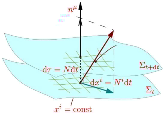
Figure 1.
Spacetime is split into three-dimensional hypersurfaces labeled by a time parameter t, with the orthonormal vector . The figure illustrates the various quantities involved in the split of the metric expansion (1).
2.1. Space and Time Decomposition: The 3 + 1 Split
In a space + time () decomposition of spacetime, the general four-dimensional metric has ten independent components, which are decomposed into a lapse function N, a shift vector , and the three-dimensional hypersurface- (-) induced metric (first fundamental form) through the following equation:2
from which one builds the second fundamental form
which is also called the extrinsic curvature of the hypersurfaces. The relevant action for GR reads, integrated over the manifold , as follows:
where , , and as Newton’s constant. This is the Einstein–Hilbert action, including in the most general situation a possible cosmological constant . We also wrote, for the sake of generality, the Gibbon–Hawking surface term3 (integrated over the boundary ), introduced by Einstein in 1916. In what follows, however, we shall restrict attention to compact hypersurfaces , for which this term identically vanishes. In (3), we also consider the possibility of a matter component, encoded as , with dynamics driven by generic fields labeled as , which is undetermined at this stage.
In terms of the decomposition stemming from (1), this action can be transformed into its Arnowitt–Deser–Misner (ADM) [12] form given by the following:
where is the Ricci scalar derived from the three-dimensional metric . The Lagrangian L thus defined permits the calculation of the canonical momenta corresponding to the underlying variables presented above in (1) and (2). These are the following:
for the purely gravitational part, and
in the case of actually representing a minimally coupled scalar field; we also used the decomposition (e.g., see Ref. [4]). We note that explicitly occurs in (5), which is why it will already appear in the vacuum equation for quantum gravity (see (15) below).
Since neither the shift vector nor the lapse time derivatives enter the Lagrangian appearing in (4), their associated momenta are vanishing and merely set the following primary constraints:
where ≈ denotes Dirac’s weak equality. With the momenta at hand, one thus finds the gravitational part of the Hamiltonian (i.e., setting ):
where
and
When adding the matter part, picks a part proportional to the energy density , while contains the current . It is then clear from (8) that Hamilton’s equations imply the Hamiltonian and the diffeomorphism (momentum) constraints, which, together with the six dynamical equations for , provide the canonical form of GR that is entirely equivalent to the ten Einstein equations.
The constraints (9) and (10) obey a certain algebra which is closed but not a Lie algebra [4]. The reason why this is not a Lie algebra is the explicit occurrence of the (inverse) three-metric in the Poisson bracket between (9) evaluated at different space points, which in turn originates from the constraint algebra not being the algebra of spacetime diffeomorphisms. Generators for those diffeomorphisms necessarily employ the lapse and the shift functions (for example, see Ref. [13]). For this reason, observables in GR (and in other diffeomorphism-invariant theories) are supposed to commute (in the sense of Poisson brackets) with a gauge generator that consists of a tuned sum of all constraints, including the primary constraints (7) together with lapse and shift [13,14]. This is why observables in GR are not necessarily constants of motion because they do not need to commute separately with the Hamiltonian and momentum constraints (as is sometimes claimed in the literature).
2.2. Superspace and Canonical Quantization
The most straightforward way to quantization once the Hamiltonian formalism has been established consists, first of all, in defining the relevant configuration space. In the case of GR, we have seen that the relevant dynamical variables are the three-metric components and the matter fields jointly described by a single symbol . All these depend on a coordinate parameterization on the three-surface , labeled by . In other words, we begin with the space:
The space is, however, too large as it contains many equivalent configurations, namely those that can be related by (three-dimensional) diffeomorphisms. Denoting by the set of all such possible diffeomorphisms, one ends up taking into account GR-invariance by reducing it to the configuration space as the quotient:
an actual configuration consisting in the equivalence class of the three-dimensional metric and field . With these configurations, one can consider a set of states of the space “Conf”, called superspace, onto which one can project a relevant state to yield the equivalent of the “position” representation for the wave function, here replaced by the wave functional:
It is not clear whether the ensemble can actually be built explicitly or even defined, and the above definition is merely suggestive in order to draw an analogy with ordinary quantum mechanics [15]. For a detailed discussion of these concepts, we refer the reader to Ref. [16].
The equations satisfied by the wave function are then obtained by applying the Dirac quantization procedure, in which the metric and fields are merely multiplicative operators, and the momenta read as follows:
for the relevant degrees of freedom, and for the primary constraints, the latter reading on the following state:
expressing, as anticipated in Equation (11), that depends neither on the lapse N nor on the shift .4 With the prescription (12), one transforms the momentum constraint (10)—now including the matter part—into the following equation:
which can be understood to mean that configurations related by a coordinate transformation yield similar wave functionals; more precisely, wave functionals remain invariant under three-dimensional diffeomorphisms connected with the identity and acquire a phase for non-connected (“large”) ones. Finally, the Hamiltonian constraint (9)—also including the matter part—yields the equation below:
with the DeWitt metric given by the following:
Equation (15) is called the Wheeler–DeWitt equation. In the way it is written here, it only has formal significance because we do not give a mathematical definition for the second functional derivatives with respect to the three-metric. This is connected to the factor-ordering problem and requires employing a regularization and (perhaps) renormalization. There is no consensus on how this can be achieved, although there are concrete proposals in the literature [17]. Only if these technical problems are solved can we also investigate whether an anomaly-free version of the classical constraint algebra mentioned above can be formulated.
The Wheeler–DeWitt Equation (15) takes the form of a stationary Schrödinger equation with an energy value of zero. This points to the absence of time at the most fundamental level and will be discussed in the next section. An important remark concerning the structure of (15) is the fact that the signature of its kinetic term is indefinite. More precisely, the DeWitt metric can be interpreted as a symmetric matrix (at each space point), which can be diagonalized to finding the signature . The minus sign is unrelated to the Lorentzian structure of classical spacetime; it is a consequence of the attractive nature of gravity [4,16]. The minus sign is connected to the local scale (“local volume”) and gives Equation (15) the structure of a locally hyperbolic (Klein–Gordon type of) equation. The variable connected to this sign may thus be interpreted as an intrinsic time—time that is entirely constructed from components of the three-metric. Julian Barbour has emphasized the analogy of such an intrinsic time with the ephemeris time used by astronomers in the past [18].
We emphasize again that the formalism of quantum geometrodynamics is a very conservative one. The Wheeler–DeWitt equation and the momentum constraints follow in a straightforward way when we take Schrödingers route of 1926, that is, “guessing” wave equations that, in the classical limit, lead back to Einstein equations in Hamilton–Jacobi form.
3. The Question of Time
It is common knowledge that the physicists’ view of time evolved in 1905 when Einstein made it relative to each observer, that is, when he introduced the notion of proper time. But special relativistic time is still an absolute concept as it relies on a set of privileged inertial frames stemming from the existence of Killing vectors in Minkowski space, which provides a fixed (non-dynamical) background. In contrast, spacetime is dynamical in GR, and an arbitrary spacetime does not possess any timelike Killing vector. In that sense, it seriously departs from what is needed in quantum mechanics.
3.1. Classical Time
A major feature of GR is its background independence. This means that all variables are dynamical, and absolute structures have disappeared. In Einstein’s words [19], here in Jürgen Ehlers’ translation [10]:5
It is contrary to the scientific mode of understanding to postulate a thing that acts, but which cannot be acted upon.
This background independence is sometimes referred to as the problem of time in the classical theory, although in our opinion, it is not a problem but a main, if not the main, feature of GR.
The canonical form of GR is very much suited to explicitly exhibit its dynamical structure. This is achieved by formulating “interconnection theorems” that demonstrate how equations on three-dimensional hypersurfaces are connected with spacetime equations (for example, see Ref. [20] and references therein).
One theorem states the following connection: the constraints and (which are four out of the ten Einstein equations), as imposed on an “initial hypersurface”, are preserved in time if and only if the energy–momentum tensor of matter has vanishing covariant divergence. This has a nice analogy in electrodynamics: the Gauss constraint is preserved if and only if there is charge conservation. A second theorem states that Einstein equations are the unique propagation law consistent with the constraints, that is, if the constraints are imposed on every hypersurface, the connection between the hypersurfaces must be through the remaining six dynamical Einstein equations. Again, there is an analogy in electrodynamics: Maxwell’s equations are the unique propagation law consistent with the Gauss constraint.
Let us consider a classical system with n variables , , depending on time t. One can formulate the canonical equations in a parametric form by setting the classical time variable as and adding an external parameter such that , with , and . The action integral then transforms into the following:
where is a homogeneous function in , so that
(with implicit summation over ), that is, the Hamiltonian associated with the system including time as a variable vanishes identically. Switching back to the original variables t and its associated momentum , one finds that implies , where H is the original Hamiltonian derived from the Lagrangian L. Interpreting this equation as a constraint equation on the full (unconstrained) phase space, one can reformulate it using Dirac’s weak equality: . In the next subsection, we shall see that the quantum version of this constraint is just the Schrödinger equation.
In GR, one could hope that through a canonical transformation, the six geometric variables can be split into four embedding coordinates of the hypersurface , say, and two actual gravitational degrees of freedom (which in the linearized limit could be interpreted as the two helicity states of weak gravitational waves). Similarly to the parametric form above, one could hope that the vanishing Hamiltonian (9) could be expanded to a form similar to , with H depending only on the relevant degrees of freedom; in that case, the Wheeler–DeWitt Equation (15) would exhibit a time structure similar to the one in the Schrödinger equation, with time interpreted as an internal degree of freedom. It so happens that in some simple cases (e.g., a Friedmann universe with matter content dominated by a barotropic perfect fluid or a Bianchi I model in vacuum), one may identify some variable to serve as such clocks. Unfortunately, in general, such a separation is not globally feasible as time in GR is very much intertwined with all other variables; this is called the global problem of time [1]. Even if such a separation can be shown to exist in particular cases, it is hard to perform it explicitly, and even if it can be accomplished, the resulting equations can hardly be solved. This is why this “reduced approach” has not proven to be a viable one in dealing with the problem of time.
This is different from the situation in classical mechanics. There, one can artificially re-write the equations in a reparametrization-invariant way. The standard Newtonian time t then follows the demand to have the equations as simple as possible. Or, in the words of Henri Poincaré [21] (our translation from French):6
Time must be defined in such a way that the equations of mechanics are as simple as possible. In other words, there is no way to measure time that is more true than any other; the one that is usually adopted is only more convenient.
This is not possible in GR—there is no distinguished time that renders the equations simple in a similar way.
3.2. Time and the Quantum
As we have seen in the last subsection, treating mechanics as a parametrized system leads to the constraint where H is the usual Hamiltonian and the momentum conjugate to t, here elevated formally to a dynamical variable. The application of Dirac’s formal quantization rules, including in particular, then leads to the Schrödinger equation:
In the standard view of quantum mechanics, t is interpreted as an external parameter (Newton’s absolute time). That the interpretation of t as an operator (“q-number”) leads to problems was already recognized by the pioneers of the theory. Wolfgang Pauli, in his textbook on quantum mechanics, emphasizes that the presence of an operator t obeying a canonical commutation rule with the Hamiltonian would lead to having a spectrum from to . He writes [22], p. 60 (our translation from German):7
We thus conclude that one must completely go without the introduction of an operator t and that the time t in wave mechanics must necessarily be considered as an ordinary number (“c-number”).
Erwin Schrödinger, in Ref. [23], p. 243, emphasizes (our translation from German):8
One can arrive at an empirical knowledge of the time variable by no other means than by a real reading of a really existing clock. This clock is a physical system like any other, and the reading of the pointer is a physical measurement like any other. It is not acceptable to put this particular physical system and this particular kind of measurements, as we may say, hors concours, and to apply the principles of quantum mechanics only to all others but not to the determination of time.
Schrödinger then proceeds to show that it is impossible to construct a time operator whose eigenvalues monotonically correlate with t if one demands a bounded Hamiltonian. In more recent years, the conclusions by Pauli and Schrödinger were re-formulated and strengthened, e.g., in Ref. [24].
One can, of course, try to re-formulate quantum mechanics by replacing the Schrödinger Equation (16) with an equation that does not refer to the external t, but to a variable describing a real clock [25]. Such an approach is realized in the “Montevideo interpretation” of quantum theory [26]. One finds in this way a master equation of the Lindblad type for an effective density matrix, which does not evolve unitarily.
Schrödinger claimed that this conceptual problem can only be solved by developing a relativistic framework. As we have seen, the background independence of GR brings this discussion to a new level and leads, after quantization, to the quantum version of the problem of time, to which we now turn.
3.3. The Problem
We have seen that one can understand GR as that which provides (generalized) trajectories of three-dimensional space, in much the same way as usual classical mechanics provides particle trajectories. Spacetime can be interpreted as a class of trajectories in the space . Since the classical particle trajectories are absent in quantum mechanics, one expects that the same applies to spacetime in quantum gravity. In fact, this is what the application of the standard quantization rules, as reviewed above, gives. Figure 2, which is a modified and extended version of Box 43.1 in Ref. [27], presents a comparison of geometrodynamics with particle dynamics, from which it becomes clear that the quantum states can be represented by wave functionals on the space of three-geometries, not four-geometries.
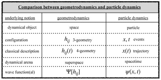
Figure 2.
Geometrodynamics shares many properties with particle dynamics, and the relevant notions in both can be compared as shown. Modified and extended version of Box 43.1 in Ref. [27].
Therefore, at the fundamental level, spacetime (and with it, time) has disappeared, and only space remains. This consequence holds for any theory that is reparametrization-invariant at the classical level. As mentioned above, it is generally not possible to consistently rewrite the constraint equations of GR in a form similar to . All momenta in the Wheeler–DeWitt Equation (15) appear quadratically, and there is no distinguished part of the momenta that may serve as being conjugate to a distinguished time. In this sense, the classical “problem of time” (background independence) leaves its imprint on quantum theory.
The discussion presented here is based on the canonical (Hamiltonian) formalism of quantum GR. Alternatively, one can use the covariant (path-integral) formulation. At the formal level, that is, neglecting field-theoretic subtleties, the two formulations are equivalent: the path integral satisfies the Wheeler–DeWitt equation and the momentum constraints ([4], Section 5.3.4). For this reason, all issues related to the problem of time hold equally well in the covariant formulation.
In quantum mechanics, the evolution with respect to the external time t is unitary for closed systems, that is, probabilities are conserved. If time is absent, the question arises whether the concepts of probability and unitarity still make sense. These issues are always included, at least implicitly, when addressing the problem of time.
The absence of spacetime, and with it the absence of any external time variable at the most fundamental level, is usually what is meant when one talks about the problem of time in quantum gravity and quantum cosmology. What are the suggestions for its solution?
3.4. Two Solutions
We present here two main solutions to address the problem of time. For a comprehensive review on potential solutions, we recommend Ref. [6] and the 933 references therein.
3.4.1. Intrinsic Time
The most straightforward approach is to accept the absence of spacetime at the fundamental level and to search for an interpretation that is solely based on three-metrics (and -geometries). The standard concept of time then only emerges at an appropriate semiclassical limit (see Section 3.5 below). The semiclassical limit is in any case demanded for consistency and is all that is presently available for experimental or observational tests.
As we have already mentioned above, the Wheeler–DeWitt Equation (15) is of a locally hyperbolic form, with the local scale coming with a different sign in the kinetic term. One could then call the local scale a local intrinsic time. Intrinsic time is entirely constructed from spatial degrees of freedom (e.g., see Ref. [28]).
Most discussions in quantum cosmology deal, in fact, with simplified models that assume a model of a homogeneous universe. Since most degrees of freedom of the full theory are absent then (there are, in particular, no gravitational waves), one calls them minisuperspace models [29]. For simplicity, let us choose a closed Friedmann–Lemaître universe with scale factor a, containing a homogeneous massive scalar degree of freedom ; this gives a two-dimensional configuration space. Classically, the line element reads as follows:
where is the standard line element on the three-sphere. The quantum version invokes a wave function depending on the two variables, . The momentum constraints are identically fulfilled, and the Wheeler–DeWitt equation reads as follows (in units where ):
Here, the factor ordering is chosen in order to achieve covariance in minisuperspace.
The hyperbolic structure is obvious from (18): the kinetic term for the scale factor has a different sign. That this sign is connected with a and not with can be recognized by adding further degrees of freedom, for example, shape degrees and additional matter fields.
The structure of (18) gives rise to two drastically different types of determinism in the classical and quantum theory [4,30] (see Figure 3 below, taken from [4]). In the classical theory, we have a trajectory in the -configuration space found by imposing initial conditions at one side of the trajectory (e.g., near the “big bang”). For a recollapsing universe, the collapsing part of the trajectory can be considered as the deterministic successor of the expanding part; “big crunch” is different from “big bang”.
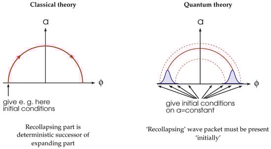
Figure 3.
Comparison between classical trajectory and the quantum wavefunction for a classically expanding and collapsing universe.
It is not so in quantum theory. For the wave Equation (18), initial conditions must be formulated at constant a. In order to construct a wave packet following the classical trajectory as a narrow tube, the initial condition at constant has to include both the “big bang” piece and the “big crunch” piece; in configuration space, they are both part of constant. The quantum determinism acts from small a to large a, not along a classical trajectory (which is absent).
This new type of determinism in quantum cosmology has important consequences when discussing the origin of the arrow of time [30]. For an initial condition of small entropy at small scale factor, the arrow of time would formally reverse at the classical turning point [31]. The reason for this is that small entropy at small a would refer to both the “big bang” piece and the “big crunch” piece of the wave packet; entropy would increase with increasing a and not along a classical trajectory (classical spacetime). A low initial entropy could come from a quantum version of Penrose’s Weyl curvature hypothesis [32]. Quantum geometrodynamics is able to implement the avoidance of cosmic singularities by invoking DeWitt’s criterion [33]: regions in configuration space are avoided in quantum gravity if the wave function vanishes there. This criterion can be generalized to accommodate the conformal structure of the configuration space [34]. With this, singularity avoidance has been shown for isotropic and anisotropic models (for example, see Refs. [34,35] and the references therein). These insights demonstrate the importance of a thorough understanding of the concept of time in quantum cosmology.
As is well known, there is still an ongoing debate about the interpretation of quantum theory. The situation becomes especially demanding in quantum cosmology, where by definition we are dealing with a quantum theory of a closed system, with no reference to external observers or measurement agencies. Accepting the linear nature of quantum theory and the universal validity of the superposition principle, one natural way would be to invoke the Everett or “many worlds” interpretation.9 Bryce DeWitt, in his pioneering paper on canonical quantum theory, writes [33]:
Everett’s view of the world is a very natural one to adopt the quantum theory of gravity, where one is accustomed to speak without embarassment of the ‘wave function of the universe.’ It is possible that Everett’s view is not only natural but essential.
It has indeed become possible to speak without embarassment of the wave function of the universe [15]. It is no coincidence that Everett’s interpretation became more wildly known only after DeWitt had made use of it in quantum cosmology. In the next subsection, we discuss a different approach to interpreting quantum cosmology and the problem of time.
3.4.2. The Trajectory Approach
As one way to understand the problem of time consists in arguing that one cannot reconstruct a four-dimensional spacetime from a given three-dimensional initial hypersurface because of the lack of dynamical equations, it is natural to think that having such dynamical equations at the quantum level could actually solve the problem (note that it can also lead to new effects that could potentially be observed in a cosmological setup [36]). In the case of the Schrödinger equation, this implies particle trajectories, although not the classical ones, as suggested in 1927 by de Broglie [37] and further completed 25 years later by Bohm [38,39]. Similarly, actual functions could be obtained.
In quantum mechanics, this works as follows. By making the amplitude and phase of the wave function explicit through and setting in the Schrödinger Equation (16), one gets the following continuity equation:
and a modified Hamilton–Jacobi equation:
by splitting (16) into its real and imaginary parts. Equation (19) leads to the usual Born probability density , while the momentum can be identified with ; the classical potential is then seen to be corrected by a quantum potential Q given by the following:
Assuming now an actual trajectory , the momentum can be written as , thereby defining a velocity that satisfies the following guidance equation:
which induces a quantum correction to the classical evolution. Note that it also naturally provides a clear distinction between the classical and the quantum regimes, the former being recovered in the limit , a well-defined and state-dependent statement.
Let us restrict our attention to a minisuperspace model, in which one formally replaces with a simpler three-metric , including symmetries (e.g., homogeneity and/or isotropy) and matter content in a set standing collectively for the geometric degrees of freedom that are relevant to encode the symmetries and the variables that describe matter; in the case of (17), for instance, one would have . In terms of these variables, the DeWitt metric is reduced from to , and writing the last term in (15) containing the intrinsic scalar curvature and the 00 component of the stress tensor as a mere function V of the , the Wheeler–DeWitt equation becomes [40]:
By expanding the wave functional into amplitude and phase S once again, one gets the modified Hamilton–Jacobi equation:
whose solution yields the function , and
hence, one can identify the “velocity” through
This gives , that is, a full reconstruction of a four-dimensional spacetime. Note that with Equation (26), being invariant under time reparametrization, the resulting spacetime geometry is independent of the choice of the lapse function N, as required.
In general, however, the trajectory approach cannot really come to an absolute conclusion as to whether there exists a satisfying solution to the problem of time in quantum gravity, even though it is the case for at least the quantum cosmological setup in which one restricts attention to minisuperspace. We refer the reader to Ref. [40] and the references given therein, in which a detailed discussion of the possible wave functional configurations and their consequences is presented.
3.5. Time from Semiclassical Gravity
Since the early days of quantum theory, scientists have already speculated about the meaning of the t in the Schrödinger Equation (16). We have already referred to the work of Pauli and Schrödinger. In 1931, Neville Mott made another important contribution [41]. He proposed that it is not the time-dependent but the time-independent Schrödinger equation, , that is fundamental. The time-dependent version emerges from a correlation between subsystems in the total time-independent system.
As a concrete example, Mott considered an electron, described by position , interacting with an alpha-particle, described by position . By making the following ansatz:
he was able to derive an effective time-dependent Schrödinger equation for the electron, with time t constructed from the Z-coordinate of the alpha-particle. In this, he explicitly referred to the approximation introduced by Born and Oppenheimer in 1927. Time is thus defined by the alpha-particle. The general idea of deriving evolution entirely from internal clock readings was elaborated on in detail by Ref. [42].
A similar mechanism is at work in quantum cosmology. There, a semiclassical time can emerge from the timeless Wheeler–DeWitt equation by dividing the total system into subsystems, with one of these subsystems capable of providing a time variable in reference to which the other subsystems evolve. To be more concrete, the limit of quantum field theory in an external spacetime can be obtained by a Born–Oppenheimer type of expansion scheme with respect to the Planck-mass squared, [43]. One starts with the following ansatz for the total wave function(al) of gravity and matter:
and expands the exponent in powers of ,
This is then inserted into the full Wheeler–DeWitt equation, and different powers of are compared. The highest orders, and , lead to a -independent , for which the gravitational Hamilton–Jacobi equation holds. In this way, (vacuum) GR is recovered.10
At the order , one obtains an equation for that can be simplified by introducing the following equation:
and demanding the standard “WKB prefactor equation” for D, which is actually similar to (25). Next, one can define a local “bubble” (Tomonaga–Schwinger) time functional by:
with this, we obtain the following Tomonaga–Schwinger (local Schrödinger) equation:
where is the matter Hamiltonian density. We note that is not a scalar function because the commutator of at different space points does not vanish [44]. Nevertheless, one can integrate (30) over with a chosen lapse function to yield a (functional) Schrödinger equation with respect to a “WKB time” t and the non-gravitational part of the full Hamiltonian. This equation describes the limit of quantum field theory in curved spacetime. The next order, , gives genuine quantum-gravitational correction terms to the matter Hamiltonian.
There has been a debate about whether the Schrödinger equation with the quantum-gravitational corrections evolves unitarily or not with respect to WKB time. Since this equation is derived from the Wheeler–DeWitt equation, one would not expect that it does. One can, however, construct a physical inner product by an intricate construction in reference to which there is a unitary evolution [35]. Using these correction terms, one can unambiguously calculate quantum-gravitational corrections to the CMB power spectrum [45]. These are observable in principle but not in practice because the factor in the denominator makes them too small.
The derivation of the Schrödinger equation from the timeless Wheeler–DeWitt Equation (15) works only for complex solutions of the form (at the highest order) , with a real . The there is the same that occurs in the Schrödinger equation with respect to WKB time. It is only for such complex states that standard quantum (field) theory can be derived as an approximation from timeless quantum gravity.11 For such states, one can invoke the standard notions of probability and unitarity. In light of the full Wheeler–DeWitt equation, these are only approximate (“phenomenological”, in the words of DeWitt) notions. Such states occur in the BO-approximation discussed above, but can also be introduced beyond it [35]. One can also argue from the trajectory approach that the probability interpretation in the form of the Born rule can only emerge in the semiclassical limit [36].
General states can be found in these complex states by the application of the superposition principle. Superposing, particularly with its complex conjugate, one obtains a real (approximate) solution to the Wheeler–DeWitt equation. The notions of WKB time and unitarity can only be employed for the two complex components in this superposition provided these components decohere. Decoherence comes from the interaction between relevant and irrelevant degrees of freedom and guarantees that in most (but not all) situations usually dealt with in cosmology, the classical appearance of (most) gravitational degrees of freedom holds (for example, see Ref. [4], Chap. 10, and the references therein). The time concept discussed in Section 3.4.1 above, together with the recovery of time from semiclassical gravity discussed here, provides a minimal solution to the problem of time and is in accordance with all observations made so far.
Some final remarks are in order for isolated quantum-gravitational systems such as (quantum) black holes. For such systems, one can derive an effective Schrödinger equation in which t is the WKB time of the (semiclassical) Universe in which the black holes are embedded, but where the Hamiltonian is the Wheeler–DeWitt Hamiltonian for the quantum black hole [48]. For such isolated systems, therefore, there is no problem of time, and the standard notions of probability and unitarity apply. The problem of time is a problem for closed quantum-gravitational systems such as the Universe as a whole.
4. Conclusions
The question of time in quantum cosmology represents a serious challenge to be understood fully in order to build a complete quantum gravity theory from which the observed world, based on the classical theory of general relativity, can be derived. The ability to produce a consistent four-dimensional spacetime must indeed be ensured, a highly nontrivial task within all the known setups or approximations that have been proposed to implement its quantization. Here, we have discussed the case of canonical GR through the Wheeler–DeWitt equation, and we have shown but a few plausible solutions among many [6,49].
In spite of this restriction, we believe that aspects of the problem of time discussed in this article as well as their possible solutions can be found for a large class of quantum-gravity approaches, definitely for those approaches that arise heuristically from a formal quantization of a classically diffeomorphism-invariant theory. This is evident for all generalized geometrodynamic theories of gravity, such as -theories, which can be re-formulated as Einstein gravity plus a scalar field. An explicitly discussed example is conformal (Weyl) gravity where a concept of shape time emerges [50]. The situation is somewhat different in loop quantum gravity, which is a theory that follows from a quantization of GR, but which makes use of different variables. For this reason, the concept of time exhibits subtleties in addition to the ones discussed here for geometrodynamics (see [51] and the references therein). The situation is really different in string theory, because this is not a direct quantization of GR but a fundamental quantum theory of all interactions from where quantum gravity arises as an emergent theory. However, it is also claimed there that spacetime is not fundamental; instead, it must be constructed from a holographic, dual theory [52]. A detailed discussion of time in these more generalized theories is beyond the scope of our paper.
Author Contributions
Writing—review and editing, C.K. and P.P. All authors have read and agreed to the published version of the manuscript.
Funding
This research received no external funding.
Institutional Review Board Statement
Not applicable.
Informed Consent Statement
Not applicable.
Data Availability Statement
Not applicable.
Conflicts of Interest
The authors declare no conflict of interest.
Notes
| 1 | The origin of this discussion can, in fact, be traced back to the pioneering work of Léon Rosenfeld in 1930, see the detailed account by Salisbury in Ref. [7]. |
| 2 | We use units in which . |
| 3 | For a recent discussion of boundary terms, see Ref. [11]. |
| 4 | In the following we shall set . |
| 5 | The German original reads: “Es widerstrebt dem wissenschaftlichen Verstande, ein Ding zu setzen, das zwar wirkt, aber auf das nicht gewirkt werden kann”. |
| 6 | The French original reads: “Le temps doit être défini de telle façon que les équations de la mécanique soient aussi simples que possible. En d’autres termes, il n’y a pas une manière de mesurer le temps qui soit plus vraie qu’ une autre; celle qui est généralement adoptée est seulement plus commode”. |
| 7 | The German original reads: “Wir schließen also, daß auf die Einführung eines Operators t grundsätzlich verzichtet und die Zeit t in der Wellenmechanik notwendig als gewöhnliche Zahl (‘c-Zahl’) betrachtet werden muß”. |
| 8 | The German original reads: “Zur empirischen Kenntnis der Zeitvariablen kann man auf keine andere Weise als durch wirkliche Ablesung einer wirklich existierenden Uhr gelangen. Diese Uhr ist ein physikalisches System wie jedes andere, die Ablesung ihres Zeigerstandes eine physikalische Messung wie jede andere. Es geht nicht an, dieses eine physikalische System und diese eine Art von Messungen sozusagen hors concours zu stellen und bloß auf alle übrigen die Grundsätze der Quantenmechanik anzuwenden, auf die Zeitbestimmung aber nicht”. |
| 9 | The name “many worlds” may, strictly speaking, be inappropriate because one deals with one quantum world. In fact, Everett himself used the term “relative states”. |
| 10 | Non-vacuum GR can be recovered by adding some of the -degrees of freedom to . |
| 11 | A general discussion of why we need complex quantum states and where they come from can be found in the twin papers [46,47] and the references therein. |
References
- Kuchař, K. Time and interpretations of quantum gravity. Int. J. Mod. Phys. D 2011, 20, 3–86. [Google Scholar] [CrossRef]
- Isham, C. Canonical quantum gravity and the problem of time. In Integrable Systems, Quantum Groups, and Quantum Field Theories; Springer: Berlin, Germany, 1993; Volume 409, pp. 157–287. [Google Scholar]
- Halliwell, J. The Interpretation of quantum cosmology and the problem of time. In Proceedings of the Workshop on Conference on the Future of Theoretical Physics and Cosmology in Honor of Stephen Hawking’s 60th Birthday, Cambridge, UK, 7–10 January 2002; pp. 675–692. [Google Scholar]
- Kiefer, C. Quantum Gravity, 3rd ed.; Oxford University Press: New York, NY, USA, 2012. [Google Scholar]
- Kiefer, C. Conceptual Problems in Quantum Gravity and Quantum Cosmology. ISRN Math. Phys. 2013, 2013, 509316. [Google Scholar] [CrossRef]
- Anderson, E. The Problem of Time; Springer: Berlin, Germany, 2017; Volume 190. [Google Scholar] [CrossRef]
- Salisbury, D. Leon Rosenfeld and the challenge of the vanishing momentum in quantum electrodynamics. Stud. Hist. Philos. Sci. B 2009, 40, 363–373. [Google Scholar] [CrossRef]
- Arthur, R.T.W. Leibniz’s Theory of Time. In The Natural Philosophy of Leibniz; The University of Western Ontario Series in Philosophy of Science; Springer: Berlin, Germany, 1985; Volume 29, pp. 263–313. [Google Scholar]
- Barbour, J. Absolute or Relative Motion? Cambridge University Press: Cambridge, UK, 1989. [Google Scholar]
- Ehlers, J. Machian Ideas and General Relativity. From Newton’s Bucket to Quantum Gravity; Barbour, J., Pfister, H., Eds.; Birkhäuser: Boston, MA, USA, 1995. [Google Scholar]
- Feng, J.C.; Chakraborty, S. Weiss variation for general boundaries. arXiv 2021, arXiv:2111.06897. [Google Scholar]
- Arnowitt, A.; Deser, S.; Misner, C.W. The dynamics of general relativity. In Gravitation: An Introduction to Current Research; Witten, L., Ed.; Wiley: New York, NY, USA, 1962; pp. 227–265. [Google Scholar]
- Pons, J.M.; Salisbury, D.C.; Sundermeyer, K.A. Observables in classical canonical gravity: Folklore demystified. J. Phys. Conf. Ser. 2010, 222, 012018. [Google Scholar] [CrossRef]
- Pitts, J.B. Equivalent Theories Redefine Hamiltonian Observables to Exhibit Change in General Relativity. Class. Quantum Gravity 2017, 34, 055008. [Google Scholar] [CrossRef]
- Hartle, J.B.; Hawking, S.W. Wave Function of the Universe. Phys. Rev. D 1983, 28, 2960–2975. [Google Scholar] [CrossRef]
- Giulini, D. The Superspace of Geometrodynamics. Gen. Relativ. Gravit. 2009, 41, 785–815. [Google Scholar] [CrossRef]
- Feng, J.C. Volume average regularization for the Wheeler-DeWitt equation. Phys. Rev. D 2018, 98, 026024. [Google Scholar] [CrossRef]
- Barbour, J. The Nature of Time. arXiv 2009, arXiv:0903.3489. [Google Scholar]
- Einstein, A. Grundzüge der Relativitätstheorie; Friedrich Vieweg und Sohn: Braunschweig, Germany, 1922. [Google Scholar]
- Giulini, D.; Kiefer, C. The Canonical approach to quantum gravity: General ideas and geometrodynamics. In Approaches to Fundamental Physics; Springer: Berlin, Germany, 2007; Volume 721, pp. 131–150. [Google Scholar] [CrossRef]
- Poincaré, H. La Valeur de la Science; Flammarion: Paris, France, 1970. [Google Scholar]
- Pauli, W. Die allgemeinen Prinzipien der Wellenmechanik; Springer: Berlin, Germany, 1990. [Google Scholar]
- Schrödinger, E. Spezielle Relativitätstheorie und Quantenmechanik. Sitzungsberichte Preuss. Akad. Wiss. Phys.-Math. Kl. 1931, XII, 238–247. [Google Scholar]
- Unruh, W.G.; Wald, R.M. Time and the Interpretation of Canonical Quantum Gravity. Phys. Rev. D 1989, 40, 2598. [Google Scholar] [CrossRef]
- Małkiewicz, P.; Miroszewski, A. Internal clock formulation of quantum mechanics. Phys. Rev. D 2017, 96, 046003. [Google Scholar] [CrossRef]
- Gambini, R.; Pullin, J. The Montevideo Interpretation: How the inclusion of a Quantum Gravitational Notion of Time Solves the Measurement Problem. Universe 2020, 6, 236. [Google Scholar] [CrossRef]
- Misner, C.W.; Thorne, K.S.; Wheeler, J.A. Gravitation; W. H. Freeman: San Francisco, CA, USA, 1973. [Google Scholar]
- Małkiewicz, P.; Peter, P.; Vitenti, S.D.P. Quantum empty Bianchi I spacetime with internal time. Phys. Rev. D 2020, 101, 046012. [Google Scholar] [CrossRef]
- Misner, C.W. Minisuperspace. In Magic without Magic: John Archibald Wheeler; Klauder, J.R., Ed.; Freeman: San Francisco, CA, USA, 1972; pp. 441–473. [Google Scholar]
- Zeh, H.D. The Physical Basis of the Direction of Time, 5th ed.; Springer: Berlin, Germany, 2007. [Google Scholar]
- Kiefer, C.; Zeh, H. Arrow of time in a recollapsing quantum universe. Phys. Rev. D 1995, 51, 4145–4153. [Google Scholar] [CrossRef] [PubMed]
- Kiefer, C. On a Quantum Weyl Curvature Hypothesis. arXiv 2021, arXiv:2111.02137. [Google Scholar]
- DeWitt, B.S. Quantum Theory of Gravity. 1. The Canonical Theory. Phys. Rev. 1967, 160, 1113–1148. [Google Scholar] [CrossRef]
- Kiefer, C.; Kwidzinski, N.; Piontek, D. Singularity avoidance in Bianchi I quantum cosmology. Eur. Phys. J. C 2019, 79, 686. [Google Scholar] [CrossRef]
- Chataignier, L. Construction of quantum Dirac observables and the emergence of WKB time. Phys. Rev. D 2020, 101, 086001. [Google Scholar] [CrossRef]
- Valentini, A. Quantum gravity and quantum probability. arXiv 2021, arXiv:2104.07966. [Google Scholar]
- De Broglie, L. La mécanique ondulatoire et la structure atomique de la matière. J. Phys. Radium 1927, 8, 225–241. [Google Scholar] [CrossRef]
- Bohm, D. A Suggested interpretation of the quantum theory in terms of hidden variables. 1. Phys. Rev. 1952, 85, 166–179. [Google Scholar] [CrossRef]
- Bohm, D. A Suggested interpretation of the quantum theory in terms of hidden variables. 2. Phys. Rev. 1952, 85, 180–193. [Google Scholar] [CrossRef]
- Pinto-Neto, N.; Struyve, W. Bohmian quantum gravity and cosmology. arXiv 2018, arXiv:1801.03353. [Google Scholar]
- Mott, N.F. On the theory of excitation by collision with heavy particles. Proc. Camb. Philos. Soc. 1931, 27, 553–560. [Google Scholar] [CrossRef]
- Page, D.N.; Wootters, W.K. Evolution without evolution: Dynamics described by stationary observables. Phys. Rev. D 1983, 27, 2885. [Google Scholar] [CrossRef]
- Kiefer, C.; Singh, T.P. Quantum gravitational corrections to the functional Schrödinger equation. Phys. Rev. D 1991, 44, 1067–1076. [Google Scholar] [CrossRef]
- Giulini, D.; Kiefer, C. Consistency of semiclassical gravity. Class. Quantum Gravity 1995, 12, 403–412. [Google Scholar] [CrossRef][Green Version]
- Chataignier, L.; Krämer, M. Unitarity of quantum-gravitational corrections to primordial fluctuations in the Born-Oppenheimer approach. Phys. Rev. D 2021, 103, 066005. [Google Scholar] [CrossRef]
- Barbour, J.B. Time and complex numbers in canonical quantum gravity. Phys. Rev. D 1993, 47, 5422–5429. [Google Scholar] [CrossRef]
- Kiefer, C. Topology, decoherence, and semiclassical gravity. Phys. Rev. D 1993, 47, 5414–5421. [Google Scholar] [CrossRef]
- Kiefer, C.; Marto, J.; Vargas Moniz, P. Indefinite oscillators and black-hole evaporation. Ann. Phys. 2009, 18, 722–735. [Google Scholar] [CrossRef][Green Version]
- Oriti, D. The complex timeless emergence of time in quantum gravity. arXiv 2021, arXiv:2110.08641. [Google Scholar]
- Kiefer, C.; Nikolic, B. Notes on semiclassical Weyl gravity. Fundam. Theor. Phys. 2017, 187, 127–143. [Google Scholar] [CrossRef]
- Rovelli, C. Space and Time in Loop Quantum Gravity. In Beyond Spacetime; Huggett, N., Matsubara, K., Wüthrich, C., Eds.; Cambridge University Press: Cambridge, UK, 2020; pp. 117–132. [Google Scholar] [CrossRef]
- Horowitz, G.T. Spacetime in string theory. New J. Phys. 2005, 7, 201. [Google Scholar] [CrossRef][Green Version]
Publisher’s Note: MDPI stays neutral with regard to jurisdictional claims in published maps and institutional affiliations. |
© 2022 by the authors. Licensee MDPI, Basel, Switzerland. This article is an open access article distributed under the terms and conditions of the Creative Commons Attribution (CC BY) license (https://creativecommons.org/licenses/by/4.0/).