The CMB, Preferred Reference System, and Dragging of Light in the Earth Frame

Abstract

The dominant CMB dipole anisotropy is a Doppler effect due to a particular motion of the solar system with a velocity of 370 km/s. Since this derives from peculiar motions and local inhomogeneities, one could meaningfully consider a fundamental frame of rest $\mathsf{\Sigma }$ associated with the Universe as a whole. From the group properties of Lorentz transformations, two observers, individually moving within $\mathsf{\Sigma }$, would still be connected by the relativistic composition rules. However, the ultimate implications could be substantial. Physical interpretation is thus traditionally demanded in order to correlate some of the dragging of light observed in the laboratory with the direct CMB observations. Today, the small residuals—from those of Michelson–Morley to present experiments with optical resonators—are just considered instrumental artifacts. However, if the velocity of light in the interferometers is not the same parameter “c” of Lorentz transformations, nothing would prevent a non-zero dragging. Furthermore, the observable effects would be much smaller than what is classically expected and would most likely be of an irregular nature. We review an alternative reading of experiments that leads to remarkable correlations with the CMB observations. Notably, we explain the irregular ${10}^{-15}$ fractional frequency shift presently measured with optical resonators operating in vacuum and solid dielectrics. For integration times of about 1 s and a typical Central European latitude, we also predict daily variations of the Allan variance in the range $(5÷12)·{10}^{-16}$.

1. Introduction

Soon after the discovery [1] of the Cosmic Microwave Background (CMB), it was realized that the observed temperature of the radiation should exhibit a small anisotropy as a consequence of the Doppler effect associated with the motion of the Earth [2,3] ($\beta =V/c)$:

$$T\left(\theta \right)=\frac{T_o\sqrt{1-{\beta }^2}}{1-\beta cos\theta }$$

(1)

Accurate observations with satellites in space [4,5] have shown that the measured temperature variations correspond to a motion of the solar system described by an average velocity $V\sim 370$ km/s, a right ascension $\alpha \sim {168}^{\circ }$, and a declination $\gamma \sim -7^{\circ }$, pointing approximately in the direction of the constellation Leo. This means that, if one sets $T_o\sim$ 2.725 K and $\beta \sim 0.00123$, there are angular variations of a few millikelvin:

$$\mathsf{\Delta }{T}^{\mathrm{CMB}}\left(\theta \right)\sim T_o\beta cos\theta \sim \pm 3.36\mathrm{mK}$$

(2)

These variations represent by far the largest contributions to the CMB anisotropy and are usually denoted as the kinematic dipole [6].

With this interpretation, it is natural to wonder about the reference frame in which this CMB dipole vanishes exactly, i.e., could it represent a fundamental system for relativity, as in the original Lorentzian formulation? The standard answer is that one should not confuse these two concepts. The CMB is a definite medium and sets a rest frame where the dipole anisotropy is zero. There is nothing strange in that our motion with respect to this system can be detected. In this sense, there would be no contradiction with special relativity.

However, to a good approximation, this kinematic dipole arises from the vector combination of the various forms of peculiar motion that are involved (rotation of the solar system around the center of the Milky Way, motion of the Milky Way toward the center of the Local Group, motion of the Local Group of galaxies in the direction of the Great Attractor, etc.) [5]. Therefore, since the observed CMB dipole reflects local inhomogeneities, it becomes natural to imagine a global frame of rest associated with the Universe as a whole. The isotropy of the CMB could then just indicate the existence of this fundamental system $\mathsf{\Sigma }$ that we may conventionally decide to call “ether”, but the cosmic radiation itself would not coincide with this form of ether1. Due to the group properties of Lorentz transformations, two observers S’ and S”, moving individually with respect to $\mathsf{\Sigma }$, would still be connected by a Lorentz transformation with a relative velocity parameter fixed by the standard relativistic composition rule 2. However, the ultimate consequences could be far reaching, even considering just the implications for the interpretation of non-locality in the quantum theory3.

The idea of a preferred frame finds further motivation in the modern picture of the vacuum, which is intended as the lowest-energy state of the theory. This is not trivial emptiness, but is believed to arise from the macroscopic Bose condensation process of Higgs quanta, quark-antiquark pairs, gluons, etc.; see, e.g., [15,16,17,18,19]. The hypothetical global frame could then reflect a vacuum structure that has a certain substantiality and can determine the type of relativity physically realized in nature.

Since the answer cannot be found with theoretical arguments only, the physical role of $\mathsf{\Sigma }$ is thus traditionally postponed to the experimental observation, in the Earth frame $S^{\prime }$, of some dragging of light: the effect of an “ether drift”. This would require: (i) the detection of a small angular dependence $\frac{\mathsf{\Delta }{\overline{c}}_{\theta }}{c}\ne 0$ of the two-way velocity of light in the laboratory and (ii) the correlation this angular dependence with the direct CMB observations with satellites in space.

Of course, experimental evidence for both the undulatory and corpuscular aspects of radiation has substantially modified the consideration of an ether and its logical need for the physical theory. However, the existence of a rest frame that is tight with respect to the underlying energy structure of the vacuum does not contradict the basic tenets of general relativity, where the off-diagonal components $g_{0i}$ of the metric play the role of a velocity field and, as such, are the most natural way to introduce effects associated with the state of motion of the observer, such as, for instance, a small angular dependence of the velocity of light4.

So far, it is generally believed that no genuine ether drift has ever been observed. In this traditional view, which dates back to the end of 19th century, when one was still comparing with Maxwell’s classical predictions for the orbital velocity $v_{\mathrm{orb}}=$ 30 km/s, all measurements (from Michelson–Morley to the most recent experiments with optical resonators) are seen as a long sequence of null results, i.e., typical instrumental effects in experiments with better and better systematics (see, e.g., Figure 1 of Ref. [25]).

However, upon closer inspection, things are not so simple for at least three reasons:

(i) In the old experiments (Michelson–Morley, Miller, Tomaschek, Kennedy, Illingworth, Piccard–Stahel, Michelson–Pease–Pearson, Joos) [26,27,28,29,30,31,32,33,34,35], light was propagating in gaseous media, air, or helium at room temperature and atmospheric pressure. In these systems with a refractive index of $\mathcal{N}=1+ϵ$, the velocity of light in the interferometers, say $c_{\gamma }$, is not the same parameter c of Lorentz transformations. Hence, nothing prevents a non-zero effect because, when light is absorbed and re-emitted, the small fraction of refracted light could keep track of the velocity of matter with respect to the hypothetical $\mathsf{\Sigma }$ and produce a direction-dependent refractive index. Then, from symmetry arguments valid in the $ϵ\to 0$ limit [36,37,38,39,40], one would expect $\frac{|\mathsf{\Delta }{\overline{c}}_{\theta }|}{c}\sim ϵ(v^2/c^2)$, which is much smaller than the classical expectation $\frac{|\mathsf{\Delta }{\overline{c}}_{\theta }{|}_{\mathrm{class}}}{c}\sim (v^2/2c^2)$. For instance, in the old experiments in air (at room temperature and atmospheric pressure, where $ϵ\sim 2.8·{10}^{-4}$), a typical value was $\frac{|\mathsf{\Delta }{\overline{c}}_{\theta }{|}_{\exp }}{c}\sim 3·{10}^{-10}$. This was classically interpreted as a velocity of 7.3 km/s, but would now correspond to 310 km/s. Analogously, in the old experiment in gaseous helium (at room temperature and atmospheric pressure, where $ϵ\sim 3.3·{10}^{-5}$), a typical value was $\frac{|\mathsf{\Delta }{\overline{c}}_{\theta }{|}_{\exp }}{c}\sim 2.2·{10}^{-11}$. This was classically interpreted as a velocity of 2 km/s, but would now correspond to 240 km/s. Those old measurements could thus become consistent with the motion of the Earth in the CMB.

(ii) Differently from those old measurements, in modern experiments, light now propagates in a high vacuum or in solid dielectrics, often in the cryogenic regime. Then, the more stringent limits of the present might not depend only on the technological progress, but also on the media that are tested, thus preventing a straightforward comparison.

(iii) In the analysis of the data, the hypothetical signal of the drift was always assumed to be a regular phenomenon—namely, with only smooth time modulations that depend deterministically on the rotation of the Earth (and its orbital revolution). The data, instead, always had an irregular behavior, with statistical averages much smaller than the individual measurements, inducing one to interpret the measurements as typical instrumental artifacts. However, a relation, if any, between the macroscopic motion of the Earth and the microscopic propagation of light in the laboratory depends ultimately on the nature of the physical vacuum. By comparing with the motion of a body in a fluid, this traditional view corresponds to the form of regular (“laminar”) flow in which global and local velocity fields coincide. Some general arguments (see [41,42]) suggest instead that the physical vacuum might behave as a stochastic medium that resembles a turbulent fluid in which large-scale and small-scale flows are only indirectly related. This means that the projection of the global velocity field at the site of the experiment, say ${\tilde{v}}_{\mu }\left(t\right)$, could differ non-trivially from the local field $v_{\mu }\left(t\right)$, which determines the direction and magnitude of the drift in the plane of the interferometer. In particular, if turbulence becomes isotropic at the small scale of the experiment, a genuine non-zero signal can coexist with vanishing statistical averages for all vector quantities. Thus, one should Fourier analyze the data for $\frac{\mathsf{\Delta }{\overline{c}}_{\theta }\left(t\right)}{c}$ and extract the (second-harmonic) phase ${\theta }_2\left(t\right)$ and amplitude $A_2\left(t\right)$, which give, respectively, the direction and magnitude of the local drift, and concentrate on the amplitude, which, being positive definite, remains non-zero under any averaging procedure. By correlating the local $v_{\mu }\left(t\right)$ with the global ${\tilde{v}}_{\mu }\left(t\right)$, the time modulations of the statistical average ${\langle A_2\left(t\right)\rangle }_{\mathrm{stat}}$ will then give information on the magnitude, right ascension, and declination of the cosmic motion. Depending on the type of correlation, there are various implications. For instance, in a uniform-probability model, where the kinematic parameters of the global ${\tilde{v}}_{\mu }\left(t\right)$ are just used to fix the typical boundaries for a local random $v_{\mu }\left(t\right)$, one finds ${\langle A_2\left(t\right)\rangle }_{\mathrm{stat}}=({\pi }^2/18){\tilde{A}}_2\left(t\right)$, where ${\tilde{A}}_2\left(t\right)$ is the amplitude in the deterministic picture. With such smaller statistical averages, one will obtain a velocity that is larger by $\sqrt{18/{\pi }^2}\sim$ 1.35 from the same data. Therefore, by returning to those old measurements—$\frac{|\mathsf{\Delta }{\overline{c}}_{\theta }{|}_{\exp }}{c}\sim 3·{10}^{-10}$ and $\frac{|\mathsf{\Delta }{\overline{c}}_{\theta }{|}_{\exp }}{c}\sim 2.2·{10}^{-11}$, respectively, for air or gaseous helium at atmospheric pressure—the data can be interpreted in three different ways: (a) as 7.3 and 2 km/s in a classical picture, (b) as 310 and 240 km/s in a modern scheme and in a smooth picture of the drift, or (c) as 418 and 324 km/s in a modern scheme, but now allowing for irregular fluctuations of the signal. In this third interpretation, the average of the two values agrees very well with the CMB velocity of 370 km/s.

After having illustrated why the evidences for $\mathsf{\Sigma }$ may be much more subtle than usually believed, in Section 2, we will review the basics of these experiments and, in Section 3 and Section 4, we will review the alternative theoretical framework of [37,38,39,40]. This will be applied in Section 5 to the old experiments in gaseous media, where $\frac{\mathsf{\Delta }{\overline{c}}_{\theta }}{c}$ was extracted from the fringe shifts in Michelson interferometers. As we will show, our scheme leads to a consistent description of the data and to remarkable correlations with the direct CMB observations with satellites in space.

Still, the simple relation $\frac{|\mathsf{\Delta }{\overline{c}}_{\theta }|}{c}\sim ϵ(v^2/c^2)$ leaves unexplained the physical mechanisms producing the observed anisotropy in gaseous systems. As a first possibility, we have thus considered that the electromagnetic field of the incoming light could determine different polarizations in different directions in the dielectric depending on its state of motion. However, if this works in weakly bound gaseous matter, the same mechanism should also work in a strongly bound solid dielectric, where the refractivity is $({\mathcal{N}}_{\mathrm{solid}}-1)=O\left(1\right)$, and thus, it should produce a much larger $\frac{|\mathsf{\Delta }{\overline{c}}_{\theta }|}{c}\sim ({\mathcal{N}}_{\mathrm{solid}}-1)(v^2/c^2)\sim {10}^{-6}$. This is in contrast with the Shamir–Fox [43] experiment in perspex, where the observed value was smaller by orders of magnitude. Then, as an alternative possibility, in Section 6, we review the traditional thermal interpretation [44,45] of the residuals in gaseous media. The idea was that, in a weakly bound system as a gas, a small temperature difference $\mathsf{\Delta }{T}^{\mathrm{gas}}\left(\theta \right)$ of a millikelvin or so between the optical arms could induce convective currents in the gas and, in turn, angular differences in the refractive index proportional to ${ϵ}_{\mathrm{gas}}\mathsf{\Delta }{T}^{\mathrm{gas}}\left(\theta \right)/T$, where $T\sim$ 300 K is the temperature of the laboratory. In our scheme, the overall consistency of different experiments would now indicate that such $\mathsf{\Delta }{T}^{\mathrm{gas}}\left(\theta \right)$ must have a non-local origin as if the interactions with the background radiation could transfer a part of $\mathsf{\Delta }{T}^{\mathrm{CMB}}\left(\theta \right)$ in Equation (2) and bring the gas out of equilibrium. However, those old estimates were slightly too large because our analysis gave $\mathsf{\Delta }{T}^{\mathrm{gas}}\left(\theta \right)=(0.2÷0.3)$ mK. Thus, these interactions were so weak that, on average, the temperature differences induced in the optical paths were only 1/10 of the $\mathsf{\Delta }{T}^{\mathrm{CMB}}\left(\theta \right)$ in Equation (2). Nevertheless, whatever its precise value is, this typical magnitude can help with intuition. In fact, it can explain the quantitative reduction of the effect in the vacuum limit, where ${ϵ}_{\mathrm{gas}}\to 0$ and the qualitative difference with strongly bound solid dielectrics, and where such small temperature differences would mainly dissipate through heat conduction without producing any particle motion and directional refraction in the rest frame of the medium.

Most significantly, this thermal argument has an interesting predictive power. In fact, it implies that if some tiny fundamental signal were definitely detected in vacuum, then, with very precise measurements, the same signal should also show up in a solid dielectric where the non-local thermal gradient is ineffective. In Section 7, this expectation will be compared with the modern experiments, where $\frac{\mathsf{\Delta }{\overline{c}}_{\theta }}{c}$ is now extracted from the frequency shift of two optical resonators. Here, after the vector average of many observations, the present limit is a residual $\langle \frac{\mathsf{\Delta }{\overline{c}}_{\theta }}{c}\rangle ={10}^{-18}÷{10}^{-19}$. However, this just reflects the very irregular nature of the signal because its typical magnitude has a value $\frac{|\mathsf{\Delta }{\overline{c}}_{\theta }\left(t\right)|}{c}\sim {10}^{-15}$, which is about 1000 times larger. This ${10}^{-15}$ magnitude is found with vacuum resonators [46,47,48,49,50,51] made of different materials and operating at room temperature and/or in the cryogenic regime, as well as in the most precise experiment ever performed in a solid dielectric [25]. As such, it could hardly be interpreted as a spurious effect. In the same model discussed above, we are then led to the concept of a refractive index ${\mathcal{N}}_v$ for the physical vacuum, which is established in an apparatus placed on the Earth’s surface. This ${\mathcal{N}}_v$ should differ from unity at the ${10}^{-9}$ level in order to give $\frac{|\mathsf{\Delta }{\overline{c}}_{\theta }{\left(t\right)|}_v}{c}\sim ({\mathcal{N}}_v-1)(v^2\left(t\right)/c^2)\sim {10}^{-15}$, and thus, it would fit with [52], where a vacuum refractivity ${ϵ}_v=({\mathcal{N}}_v-1)\sim {10}^{-9}$ was considered. 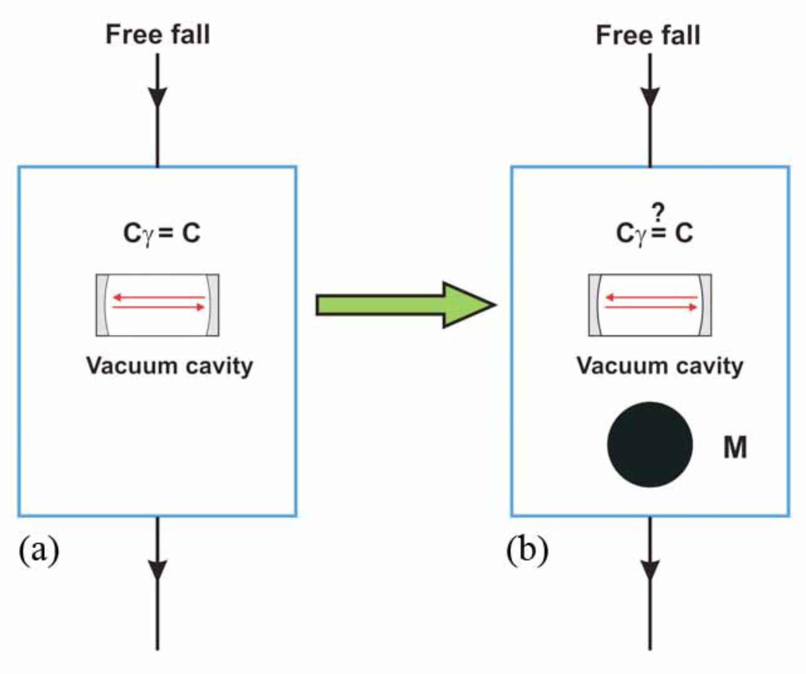Indeed, if the curvature observed in a gravitational field reflects local deformations of the physical space-time units, for an apparatus on the Earth’s surface, there might be a tiny refractivity ${ϵ}_v\sim (2G_{N}M/c^{2}R)\sim 1.4·{10}^{-9}$, where $G_N$ is the Newton constant and M and R are the mass and radius of the Earth. This could make a difference with the ideal free-fall environment, which is always assumed to operationally define the parameter c of Lorentz transformations in the presence of gravitational effects. Then, for a typical daily projection of 250 km/s $\lesssim \tilde{v}\left(t\right)\lesssim$ 370 km/s and in the same uniform-probability model that was used successfully for the classical experiments, we would expect a fundamental signal with an average magnitude of $(8.5\pm 3.5)·{10}^{-16}$. 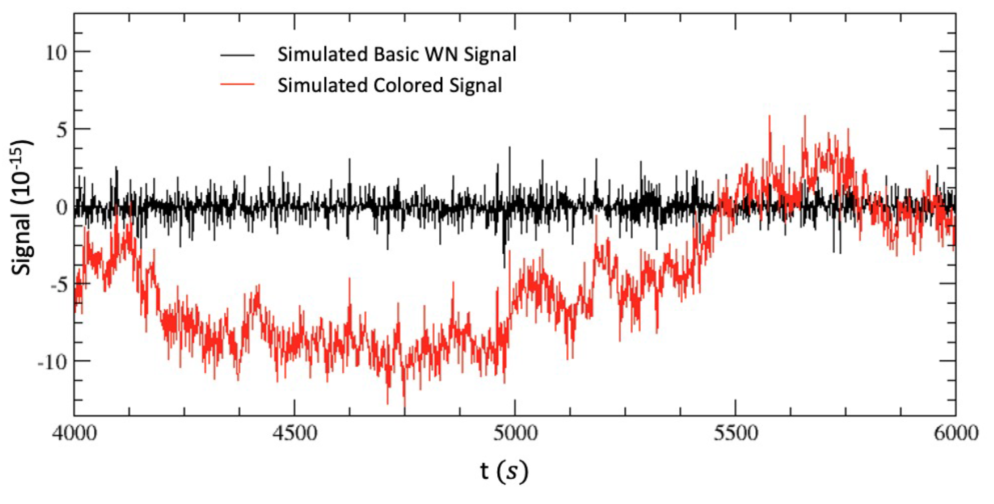This is a genuine signal, which would pose an intrinsic limitation to the precision of measurements and, according to our numerical simulations, can be approximated as white noise. Thus, it should be compared with the frequency shift of two optical resonators at the largest integration time (typically 1 s) where the pure white-noise branch is as small as possible, but other types of noise are not yet important.

As emphasized in the conclusive Section 8, the consistency of this prediction with the most precise measurements in vacuum and solid dielectrics that operate at room temperature and in the cryogenic regime and the satisfactory description of the old experiments should therefore induce one to perform an ultimate experimental check: detecting the expected, periodic, and daily variations in the range $(5÷12)·{10}^{-16}$.

2. Basics of the Ether-Drift Experiments

Let us start with some basic notions. As anticipated, old and modern experiments adopt different technologies, but, in the end, have the same scope: looking for the hypothetical $\mathsf{\Sigma }$ through a tiny angular dependence of the two-way velocity of light ${\overline{c}}_{\gamma }\left(\theta \right)$. This quantity can be measured unambiguously and is defined through the one-way velocity $c_{\gamma }\left(\theta \right)$ as

$${\overline{c}}_{\gamma }\left(\theta \right)=\frac{2c_{\gamma }\left(\theta \right)c_{\gamma }(\pi +\theta )}{c_{\gamma }\left(\theta \right)+c_{\gamma }(\pi +\theta )}$$

(3)

where $\theta$ indicates the angle between the direction where light propagates and the velocity with respect to $\mathsf{\Sigma }$. By defining the anisotropy

$$\mathsf{\Delta }{\overline{c}}_{\theta }={\overline{c}}_{\gamma }(\pi /2+\theta )-{\overline{c}}_{\gamma }\left(\theta \right)$$

one finds a simple relation with $\mathsf{\Delta }t\left(\theta \right)$, the difference in time for light propagating back and forth along perpendicular rods of length D (see Figure 1), and one finds

$$\mathsf{\Delta }t\left(\theta \right)=\frac{2D}{{\overline{c}}_{\gamma }\left(\theta \right)}-\frac{2D}{{\overline{c}}_{\gamma }(\pi /2+\theta )}\sim \frac{2D}{c}\frac{\mathsf{\Delta }{\overline{c}}_{\theta }}{c}$$

(4)

This relation was at the base of the original Michelson interferometer, but is also valid today when we assume Lorentz transformations. In this case, in fact, in the $S^{\prime }$ frame where the rod is at rest, the length D does not depend on the orientation (in the last relation, we are assuming the propagation of light in a medium with a refractive index $\mathcal{N}=1+ϵ$, and $ϵ\ll 1$). We thus get the fringe patterns ($\lambda$ being the wavelength of light)

$$\frac{\mathsf{\Delta }\lambda \left(\theta \right)}{\lambda }\sim \frac{2D}{\lambda }\frac{\mathsf{\Delta }{\overline{c}}_{\theta }}{c}$$

(5)

which were measured in the old experiments.

Instead, nowadays, an angular dependence of ${\overline{c}}_{\gamma }\left(\theta \right)$ is extracted from the frequency shift $\mathsf{\Delta }\nu \left(\theta \right)$ of two optical resonators; see Figure 2. The particular type of laser-cavity coupling used in the experiments is known in the literature as the Pound–Drever–Hall system [53,54]. The details of this technique go beyond our scope. However, the main ideas are simple and beautifully explained in Black’s tutorial article [55]. A laser beam is sent into a Fabry–Perot cavity, which acts as a filter. Then, a part of the output of the cavity is fed back to the laser to suppress its frequency fluctuations. This method provides a very narrow bandwidth and has been crucial for the precision measurements that we are going to describe.

The frequency of the resonators is proportional to ${\overline{c}}_{\gamma }\left(\theta \right)$ through an integer number m, while fixing the cavity mode and the cavity length L measured in the laboratory $S^{\prime }$ frame:

$$\nu \left(\theta \right)=\frac{{\overline{c}}_{\gamma }\left(\theta \right)m}{2L}$$

(6)

Again, by assuming Lorentz transformations, the length of the cavity in its rest frame $S^{\prime }$ does not depend on the orientation in space, so that

$$\frac{\mathsf{\Delta }\nu \left(\theta \right)}{{\nu }_0}\sim \frac{\mathsf{\Delta }{\overline{c}}_{\theta }}{c}$$

(7)

where ${\nu }_0$ is the reference frequency of the resonators. These relations have always been assumed in the interpretation of the experiments.

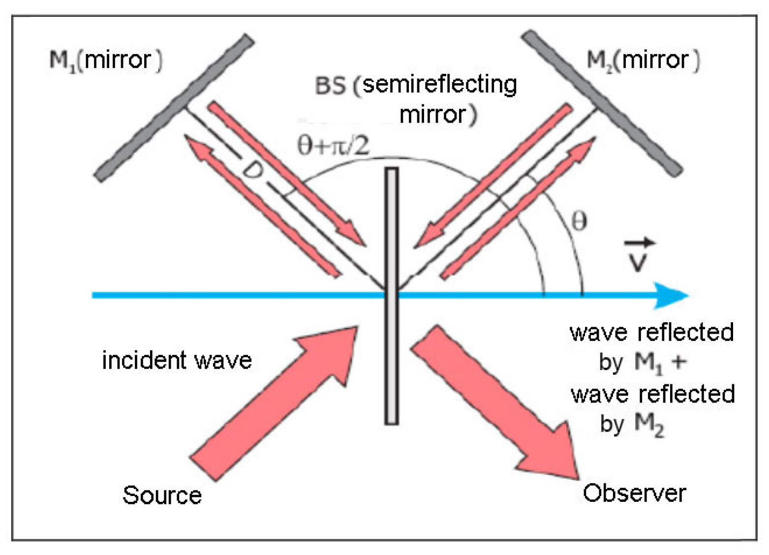
3. A Modern Version of Maxwell Calculation

For a quantitative analysis, let us consider a medium of refractive index $\mathcal{N}=1+ϵ$ with $0\le ϵ\ll 1$. This medium fills an optical cavity at rest in the laboratory $S^{\prime }$ frame in motion with velocity v with respect to $\mathsf{\Sigma }$. If we assume (a) that ${\overline{c}}_{\gamma }\left(\theta \right)$ is isotropic when $S^{\prime }\equiv \mathsf{\Sigma }$ and (b) that Lorentz transformations are valid, then any anisotropy in $S^{\prime }$ should vanish identically either for $v=0$ or for the ideal vacuum limit, i.e., when the velocity of light tends to the basic parameter c of Lorentz transformations5. Therefore, one can perform an expansion in powers of the two small parameters $ϵ$ and $\beta =v/c$. Since, by its definition, ${\overline{c}}_{\gamma }\left(\theta \right)$ is invariant under the replacement $\beta \to -\beta$ and, at fixed $\beta$, is invariant when replacing $\theta \to \pi +\theta$, the lowest non-trivial angular dependence is found to be $\mathcal{O}\left(ϵ{\beta }^2\right)$ and can be expressed in the general form [17,18,19]:

$$\begin{array}{c}\hfill {\overline{c}}_{\gamma }\left(\theta \right)\sim \frac{c}{\mathcal{N}}\left[1-ϵ{\beta }^2\sum _{n=0}^{\infty }{\zeta }_{2n}{P}_{2n}(cos\theta )\right]\end{array}$$

(8)

In the above relation, the invariance under $\theta \to \pi +\theta$ is achieved by expanding in even-order Legendre polynomials with arbitrary coefficients ${\zeta }_{2n}=\mathcal{O}\left(1\right)$. These coefficients vanish identically in Einstein’s special relativity with no preferred system, but should not vanish a priori in a “Lorentzian” formulation.

If we retain the first few $\zeta$s as free parameters, Equation (8) could already be useful for fitting experimental data. In any case, independently of their numerical values, one should appreciate the substantial difference introduced with respect to the classical prediction. As an example, by assuming, for simplicity, $v=$ 300 km/s and $ϵ\sim 2.8·{10}^{-4}$ for air at room temperature and atmospheric pressure, we find the following difference:

$$\frac{\mathsf{\Delta }{\overline{c}}_{\theta }\left(0\right)}{c}\sim 2.8·{10}^{-10}\left[\frac{3}{2}{\zeta }_2+\frac{5}{8}{\zeta }_4+\dots \right]$$

(9)

This would be about three orders of magnitude smaller than the classical estimate ${\beta }^2={10}^{-6}$ that would be expected from Maxwell’s calculation [57] for the same $v=$ 300 km/s. However, depending on the actual $\zeta$s, Equation (9) would also be about 10 ÷ 20 times smaller than the old standard value for the much lower orbital velocity $v_{\mathrm{orb}}=$ 30 km/s:

$$\frac{\mathsf{\Delta }{\overline{c}}_{\theta }\left(0\right)}{c}{|}_{\mathrm{class}}=\frac{v_{\mathrm{orb}}^2}{c^2}={10}^{-8}$$

(10)

For experiments in gaseous helium at room temperature and atmospheric pressure, where $ϵ\sim 3.3·{10}^{-5}$, the equivalent of Equation (9) would even be $100÷200$ times smaller than this old standard. The above elementary arguments suggest that the old ether-drift experiments in gaseous media might have been overlooked. So far, they have been considered as null results. However, this may just depend on a comparison with the wrong classical formula.

However, the dependence on the unknown $\zeta$s is unpleasant because it prevents a straightforward comparison with the data. For this reason, according to other symmetry arguments [37,39,40], we will further sharpen our analysis with another derivation of the $ϵ\to 0$ limit. This additional derivation makes use of the effective space-time metric $g^{\mu \nu }=g^{\mu \nu }\left(\mathcal{N}\right)$, which should be substituted into the relation $g^{\mu \nu }{p}_{\mu }{p}_{\nu }=0$ to describe light in a medium with refractive index $\mathcal{N}$; see, e.g., [58]. At the quantum level, this metric was derived by Jauch and Watson [59] when quantizing the electromagnetic field in a dielectric. They realized that the formalism introduces a preferred reference system where the photon energy $E_{\gamma }$ does not depend on the angle $\theta$ of light propagation. They observed that this is “usually taken as the system for which the medium is at rest”, a conclusion that is obvious in special relativity, where there is no preferred system, but it is less obvious in our case. We will therefore adapt their results and consider a different limit where the photon energy $E_{\gamma }$ is $\theta$—independent only when both the medium and observer are at rest in some frame $\mathsf{\Sigma }$.

To see how this works, we will consider two identical optical resonators—namely, resonator 1, which is at rest in $\mathsf{\Sigma }$, and resonator 2, which is at rest in $S^{\prime }$. We will also introduce ${\pi }_{\mu }\equiv (\frac{E_{\pi }}{c}, \mathsf{ß})$ to indicate the light 4-momentum for $\mathsf{\Sigma }$ in its cavity 1 and $p_{\mu }\equiv (\frac{E_p}{c}, \mathbf{p})$ to indicate the analogous 4-momentum of light for $S^{\prime }$ in its cavity 2. Finally, we will denote by $g^{\mu \nu }$ the space-time metric used by $S^{\prime }$ in the relation $g^{\mu \nu }{p}_{\mu }{p}_{\nu }=0$ and by

$${\gamma }^{\mu \nu }=\mathrm{diag}({\mathcal{N}}^2, -1, -1, -1)$$

(11)

the metric that $\mathsf{\Sigma }$ adopts in the analogous relation ${\gamma }^{\mu \nu }{\pi }_{\mu }{\pi }_{\nu }=0$ and that produces the isotropic velocity $c_{\gamma }=E_{\pi }/\left|\mathsf{ß}\right|=\frac{c}{\mathcal{N}}$.

We emphasize the peculiar view of special relativity where no observable difference can exist between $\mathsf{\Sigma }$ and $S^{\prime }$. In our perspective, instead, this physical equivalence is only assumed in the ideal $\mathcal{N}=1$ vacuum limit. Indeed, as anticipated in the introduction, in the presence of matter, where light is absorbed and then re-emitted, the fraction of refracted light could keep track of the particular motion of matter with respect to $\mathsf{\Sigma }$ and produce a $\mathsf{\Delta }{\overline{c}}_{\theta }\ne 0$.

By first considering the $\mathcal{N}=1$ limit, the frame-independence of the velocity of light requires one to impose

$$g^{\mu \nu }(\mathcal{N}=1)={\gamma }^{\mu \nu }(\mathcal{N}=1)={\eta }^{\mu \nu }$$

(12)

where ${\eta }^{\mu \nu }$ is the Minkowski tensor. This standard equality amounts to the introduction of a transformation matrix, say $A_{\nu }^{\mu }$, such that, for $\mathcal{N}=1$,

$$g^{\mu \nu }(\mathcal{N}=1)=A_{\rho }^{\mu }{A}_{\sigma }^{\nu }{\gamma }^{\rho \sigma }(\mathcal{N}=1)=A_{\rho }^{\mu }{A}_{\sigma }^{\nu }{\eta }^{\rho \sigma }={\eta }^{\mu \nu }$$

(13)

This relation is strictly valid for $\mathcal{N}=1$. However, by continuity, one is driven to conclude that an analogous relation between $g^{\mu \nu }$ and ${\gamma }^{\mu \nu }$ should also hold in the $ϵ\to 0$ limit. The only subtlety is that relation (13) does not uniquely fix $A_{\nu }^{\mu }$. In fact, it is fulfilled either by choosing the identity matrix, i.e., $A_{\nu }^{\mu }={\delta }_{\nu }^{\mu }$, or by choosing a Lorentz transformation, i.e., $A_{\nu }^{\mu }={\mathsf{\Lambda }}_{\nu }^{\mu }$. It thus follows that $A_{\nu }^{\mu }$ is a two-valued function when $\mathcal{N}\to 1$.

This gives two possible solutions for the metric in $S^{\prime }$. In fact, when $A_{\nu }^{\mu }$ is the identity matrix, we find

$${\left[g^{\mu \nu }\left(\mathcal{N}\right)\right]}_1={\delta }_{\rho }^{\mu }{\delta }_{\sigma }^{\nu }{\gamma }^{\rho \sigma }={\gamma }^{\mu \nu }\sim {\eta }^{\mu \nu }+2ϵ{\delta }_0^{\mu }{\delta }_0^{\nu }$$

(14)

while, when $A_{\nu }^{\mu }$ is a Lorentz transformation, we obtain

$${\left[g^{\mu \nu }\left(\mathcal{N}\right)\right]}_2={\mathsf{\Lambda }}_{\rho }^{\mu }{\mathsf{\Lambda }}_{\sigma }^{\nu }{\gamma }^{\rho \sigma }\sim {\eta }^{\mu \nu }+2ϵv^{\mu }{v}^{\nu }$$

(15)

where $v_{\mu }$ is the $S^{\prime }$ 4-velocity, and $v_{\mu }\equiv (v_0, \mathbf{v}/c)$ with $v_{\mu }{v}^{\mu }=1$. As a consequence, the equality ${\left[g^{\mu \nu }\left(\mathcal{N}\right)\right]}_1={\left[g^{\mu \nu }\left(\mathcal{N}\right)\right]}_2$ can only hold for $v^{\mu }={\delta }_0^{\mu }$, i.e., for $\mathbf{v}=0$ when $S^{\prime }\equiv \mathsf{\Sigma }$.

Notice that by choosing the first solution ${\left[g^{\mu \nu }\left(\mathcal{N}\right)\right]}_1$, which is implicitly assumed in special relativity to preserve isotropy in all reference frames, as well as for $\mathcal{N}\ne 1$, we are considering a transformation matrix $A_{\nu }^{\mu }$ that is discontinuous for any $ϵ\ne 0$. In fact, it is the non-trivial peculiarity of Lorentz transformations to enforce Equation (13) for $A_{\nu }^{\mu }={\mathsf{\Lambda }}_{\nu }^{\mu }$ so that ${\mathsf{\Lambda }}^{\mu \sigma }{\mathsf{\Lambda }}_{\sigma }^{\nu }={\eta }^{\mu \nu }$, and the Minkowski metric, if valid in one frame, will then apply to all equivalent frames.

On the other hand, if one inserts ${\left[g^{\mu \nu }\left(\mathcal{N}\right)\right]}_2$ into the relation $p_{\mu }{p}_{\nu }{g}^{\mu \nu }=0$, the photon energy $E\left(\right|\mathbf{p}|, \theta )$ will now depend on the direction of propagation. This gives the one-way velocity $c_{\gamma }\left(\theta \right)=\frac{E\left(\right|\mathbf{p}|,\theta )}{\left|\mathbf{p}\right|}$, which, to $\mathcal{O}\left(ϵ\right)$ and $\mathcal{O}\left({\beta }^2\right)$, is

$$c_{\gamma }\left(\theta \right)\sim \frac{c}{\mathcal{N}}\left[1-2ϵ\beta cos\theta -ϵ{\beta }^2(1+{cos}^2\theta )\right]$$

(16)

with a two-way combination:

$${\overline{c}}_{\gamma }\left(\theta \right)=\frac{2c_{\gamma }\left(\theta \right)c_{\gamma }(\pi +\theta )}{c_{\gamma }\left(\theta \right)+c_{\gamma }(\pi +\theta )}\sim \frac{c}{\mathcal{N}}\left[1-ϵ{\beta }^2(1+{cos}^2\theta )\right]$$

(17)

This final form, which corresponds to the setting in Equation (8) (${\zeta }_0=4/3$, ${\zeta }_2=2/3$, and all ${\zeta }_{2n}=0$ for $n>1$), could be considered the modern version of Maxwell’s calculation [57] and will be adopted in the analysis of experiments near the $ϵ=0$ limit, as for gaseous systems.

For the sake of clarity, let us return to the definition of the gas refractive index $\mathcal{N}$ in Equation (11). How is this quantity related to the experimental value ${\mathcal{N}}_{\exp }$ obtained from the two-way velocity measured in the Earth laboratory? This can be easily understood by first introducing an angle-dependent $\overline{\mathcal{N}}\left(\theta \right)$ through ${\overline{c}}_{\gamma }\left(\theta \right)\equiv c/\overline{\mathcal{N}}\left(\theta \right)$ with

$$\overline{\mathcal{N}}\left(\theta \right)\sim \mathcal{N}\left[1+(\mathcal{N}-1){\beta }^2(1+{cos}^2\theta )\right]$$

(18)

and then defining the isotropic experimental value after an angular averaging—namely,

$$\frac{c}{{\mathcal{N}}_{\exp }}\equiv {\langle \frac{c}{\overline{\mathcal{N}}\left(\theta \right)}\rangle }_{\theta }=\frac{c}{\mathcal{N}}\left[1-\frac{3}{2}(\mathcal{N}-1){\beta }^2\right]$$

(19)

One could therefore obtain the unknown value $\mathcal{N}\equiv \mathcal{N}\left(\mathsf{\Sigma }\right)$ (as if the cavity with the gas were at rest in $\mathsf{\Sigma }$) from the experimental ${\mathcal{N}}_{\exp }\equiv \mathcal{N}\left(earth\right)$ and v. As an example, the most precise determinations for air are at a level ${10}^{-7}$, say ${\mathcal{N}}_{\exp }=1.0002924\dots$, for $\lambda =$ 589 nm, 0 ${}^{°}$C, and atmospheric pressure. Therefore, for $v\sim$ 370 km/s, the difference between $\mathcal{N}\left(\mathsf{\Sigma }\right)$ and $\mathcal{N}\left(earth\right)$ is smaller than ${10}^{-9}$ and can be ignored. Analogous considerations apply to other gaseous media (such as N, CO${}_2$, helium, etc.) where the precision in ${\mathcal{N}}_{\exp }$ is, at best, at the level of a few ${10}^{-7}$. Finally, whatever v is, the relation $\mathcal{N}\left(\mathsf{\Sigma }\right)={\mathcal{N}}_{\exp }$ becomes more and more accurate in the low-pressure limit where $({\mathcal{N}}_{\exp }-1)\to 0$.

To conclude, from Equation (17), the fractional anisotropy is found to be

$$\frac{\mathsf{\Delta }{\overline{c}}_{\theta }}{c}=\frac{{\overline{c}}_{\gamma }(\pi /2+\theta )-{\overline{c}}_{\gamma }\left(\theta \right)}{c}\sim ϵ\frac{v^2}{c^2}cos2(\theta -{\theta }_2)$$

(20)

and is suppressed by the small factor $2ϵ$ with respect to the classical estimate $\frac{\mathsf{\Delta }{\overline{c}}_{\theta }}{c}\sim \frac{v^2}{2c^2}$. Here, v and ${\theta }_2$ indicate the magnitude and the direction of the drift in the interferometer’s plane, and, from Equation (5), one obtains the fringe pattern

$$\frac{\mathsf{\Delta }\lambda \left(\theta \right)}{\lambda }=\frac{2D}{\lambda }\frac{\mathsf{\Delta }{\overline{c}}_{\theta }}{c}\sim \frac{2D}{\lambda }ϵ\frac{v^2}{c^2}cos2(\theta -{\theta }_2)$$

(21)

In this way, the dragging of light in the Earth frame is described as a pure second-harmonic effect that is periodic in the range $[0, \pi ]$. This is the same as in the classical theory (see, e.g., [60]), with the exception of its amplitude,

$$A_2=\frac{2D}{\lambda }ϵ\frac{v^2}{c^2}$$

(22)

which is suppressed by the factor $2ϵ$ relative to the classical amplitude $A_2^{\mathrm{class}}=\frac{D}{\lambda }\frac{v^2}{c^2}$. This difference could then be re-absorbed into an observable velocity,

$$A_2=\frac{D}{\lambda }\frac{v_{\mathrm{obs}}^2}{c^2}$$

(23)

which depends on the gas refractive index

$$v_{\mathrm{obs}}^2\sim 2ϵv^2$$

(24)

This $v_{\mathrm{obs}}$ is the very small velocity traditionally extracted from the classical analysis of the experiments through the relation

$$v_{\mathrm{obs}}\sim 30\mathrm{km}/\mathrm{s}\sqrt{\frac{A_2^{\mathrm{EXP}}}{A_2^{\mathrm{class}}}}$$

(25)

when one was still comparing with the standard classical prediction $A_2^{\mathrm{class}}=\frac{D}{\lambda }{\left(\frac{30\mathrm{km}/\mathrm{s}}{c}\right)}^2$ for the orbital velocity.

However, before a more detailed comparison with experiments, additional considerations are needed about the physical nature of the ether drift as an irregular phenomenon. Some general motivations and a simple stochastic model will be illustrated in the following section.

4. Dragging of Light as an Irregular Phenomenon

Aside from the magnitude of the signal, the other important aspect of the experiments concerns the time dependence of the data. As anticipated in the introduction, it was always assumed that, for short-term observations of a few days where there are no sizable changes in the orbital velocity of the Earth, a genuine physical signal should reproduce the regular modulations induced by its rotation. Instead, in both classical and modern experiments, the data have always shown a very irregular behavior with statistical averages that are much smaller than the instantaneous values. This was always a strong argument for interpreting the data as instrumental artifacts. However, in principle, a definite instantaneous value $\frac{\mathsf{\Delta }{\overline{c}}_{\theta }\left(t\right)}{c}\ne 0$ could also coexist with a vanishing statistical average.

This possibility was considered in [37,38,39,40,41,42] by assuming that the observed signal is determined by a local velocity field, say $v_{\mu }\left(t\right)$, which does not coincide with the projection of the global Earth motion, say ${\tilde{v}}_{\mu }\left(t\right)$, at the observation site. By comparing with the motion of a body in a fluid, the equality $v_{\mu }\left(t\right)={\tilde{v}}_{\mu }\left(t\right)$ amounts to the assumption of a form of regular, laminar flow where global and local velocity fields coincide. Instead, in the case of a turbulent fluid, large-scale and small-scale flows would only be indirectly related.

An intuitive motivation for this turbulent-fluid analogy derives from the comparison of the vacuum to a fluid with vanishing viscosity. Then, within the Navier-Stokes equation, a laminar flow is by no means obvious due to the subtlety of the zero-viscosity (or infinite Reynolds number) limit; see, for instance, the discussion given by Feynman in Section 41.5, Volume II of his Lectures [61]. The reason is that the velocity of such a hypothetical fluid cannot be a differentiable function [62], and one should think, instead, in terms of a continuous velocity field that is not differentiable anywhere [63]. This analogy leads to the idea of a signal with a fundamental stochastic nature, such as when turbulence, at small scales, becomes homogeneous and isotropic.

With this in mind, let us return to Equation (20) and make explicit the time dependence of the signal by re-writing it as

$$\frac{\mathsf{\Delta }{\overline{c}}_{\theta }\left(t\right)}{c}\sim ϵ\frac{v^2\left(t\right)}{c^2}cos2(\theta -{\theta }_2\left(t\right))$$

(26)

where $v\left(t\right)$ and ${\theta }_2\left(t\right)$ indicate, respectively, the instantaneous magnitude and direction of the drift in the plane of the interferometer. This can also be re-written as

$$\frac{\mathsf{\Delta }{\overline{c}}_{\theta }\left(t\right)}{c}\sim 2S\left(t\right)sin2\theta +2C\left(t\right)cos2\theta$$

(27)

with

$$2C\left(t\right)=ϵ\frac{v_x^2\left(t\right)-v_y^2\left(t\right)}{c^2}2S\left(t\right)=ϵ\frac{2v_x\left(t\right)v_y\left(t\right)}{c^2}$$

(28)

and $v_x\left(t\right)=v\left(t\right)cos{\theta }_2\left(t\right)$, $v_y\left(t\right)=v\left(t\right)sin{\theta }_2\left(t\right)$.

The standard analysis is based on a cosmic velocity of the Earth characterized by a magnitude V, a right ascension $\alpha$, and an angular declination $\gamma$. These parameters can be considered constant for short-term observations of a few days so that, with the traditional identifications $v\left(t\right)\equiv \tilde{v}\left(t\right)$ and ${\theta }_2\left(t\right)\equiv {\tilde{\theta }}_2\left(t\right)$, the only time dependence should be due to the Earth’s rotation. Here, $\tilde{v}\left(t\right)$ and ${\tilde{\theta }}_2\left(t\right)$ are derived from the simple application of spherical trigonometry [64]:

$$cosz\left(t\right)=sin\gamma sin\varphi +cos\gamma cos\varphi cos(t^{\prime }-\alpha )$$

(29)

$$\tilde{v}\left(t\right)=Vsinz\left(t\right)$$

(30)

$${\tilde{v}}_x\left(t\right)=\tilde{v}\left(t\right)cos{\tilde{\theta }}_2\left(t\right)=V\left[sin\gamma cos\varphi -cos\gamma sin\varphi cos(t^{\prime }-\alpha )\right]$$

(31)

$${\tilde{v}}_y\left(t\right)=\tilde{v}\left(t\right)sin{\tilde{\theta }}_2\left(t\right)=Vcos\gamma sin(t^{\prime }-\alpha )$$

(32)

In the above relations, $z=z\left(t\right)$ is the zenithal distance of $\mathbf{V}$, $\varphi$ is the latitude of the laboratory, $t^{\prime }={\omega }_{\mathrm{sid}}t$ is the sidereal time of the observation in degrees (${\omega }_{\mathrm{sid}}\sim \frac{2\pi }{{23}^h{56}^{\prime }}$), and the angle ${\tilde{\theta }}_2\left(t\right)$ is counted conventionally from North through East so that North is ${\tilde{\theta }}_2=0$ and East is ${\tilde{\theta }}_2={90}^{\circ }$. With the identifications $v\left(t\right)\equiv \tilde{v}\left(t\right)$ and ${\theta }_2\left(t\right)\equiv {\tilde{\theta }}_2\left(t\right)$ (or, equivalently, $v_x\left(t\right)={\tilde{v}}_x\left(t\right)$ and $v_y\left(t\right)={\tilde{v}}_y\left(t\right)$), one thus arrives at the simple Fourier decomposition

$$S\left(t\right)\equiv \tilde{S}\left(t\right)=S_0+S_{s1}sin{t}^{\prime }+S_{c1}cos{t}^{\prime }+S_{s2}sin\left(2t^{\prime }\right)+S_{c2}cos\left(2t^{\prime }\right)$$

(33)

$$\begin{array}{c}\hfill C\left(t\right)\equiv \tilde{C}\left(t\right)=C_0+C_{s1}sin{t}^{\prime }+C_{c1}cos{t}^{\prime }+C_{s2}sin\left(2t^{\prime }\right)+C_{c2}cos\left(2t^{\prime }\right)\end{array}$$

(34)

where the $C_k$ and $S_k$ Fourier coefficients depend on the three parameters $(V,\alpha ,\gamma )$ and are given explicitly in [37,40].

Instead, we will consider an alternative scenario where $v_x\left(t\right)\ne {\tilde{v}}_x\left(t\right)$ and $v_y\left(t\right)\ne {\tilde{v}}_y\left(t\right)$. In particular, the local velocity components, $v_x\left(t\right)$ and $v_y\left(t\right)$, will be assumed to be non-differentiable functions expressed in terms of random Fourier series [62,65,66]. The simplest model corresponds to a turbulence, which, at small scales, appears homogeneous and isotropic. The analysis of the previous section can then be embodied in an effective space-time metric for light propagation

$$g^{\mu \nu }\left(t\right)\sim {\eta }^{\mu \nu }+2ϵv^{\mu }\left(t\right)v^{\nu }\left(t\right)$$

(35)

where $v_{\mu }\left(t\right)$ is a random 4-velocity field that describes the drift and whose boundaries depend on the smooth ${\tilde{v}}_{\mu }\left(t\right)$ determined by the average motion of the Earth. If this corresponds to the actual physical situation, a genuine stochastic signal can easily become consistent with average values ${\left(C_k\right)}^{\mathrm{avg}}={\left(S_k\right)}^{\mathrm{avg}}=0$ obtained by fitting the data with Equations (33) and (34).

For homogeneous turbulence, a series representation that is suitable for numerical simulations of a discrete signal can be expressed in the form:

$$v_x\left(t_k\right)=\sum _{n=1}^{\infty }\left[x_n\left(1\right)cos{\omega }_n{t}_k+x_n\left(2\right)sin{\omega }_n{t}_k\right]$$

(36)

$$v_y\left(t_k\right)=\sum _{n=1}^{\infty }\left[y_n\left(1\right)cos{\omega }_n{t}_k+y_n\left(2\right)sin{\omega }_n{t}_k\right]$$

(37)

Here, ${\omega }_n=2n\pi /T$, and T is the common period of all Fourier components. Furthermore, $t_k=(k-1)\mathsf{\Delta }t$, with $k=1,2\dots$, and $\mathsf{\Delta }t$ is the sampling time. Finally, $x_n(i=1,2)$ and $y_n(i=1,2)$ are random variables with the dimension of a velocity and vanishing mean.

In our simulations, the value $T=T_{\mathrm{day}}$ = 24 h and a sampling step $\mathsf{\Delta }t=$ 1 s were adopted. However, the results would remain unchanged by any rescaling of $T\to sT$ and $\mathsf{\Delta }t\to s\mathsf{\Delta }t$.

In general, we define $[-d_x\left(t\right), d_x\left(t\right)]$ as the range for $x_n(i=1,2)$ and $[-d_y\left(t\right), d_y\left(t\right)]$ as the corresponding range for $y_n(i=1,2)$. By assuming statistical isotropy, we should impose $d_x\left(t\right)=d_y\left(t\right)$. However, to see the difference, we will first consider the more general case of $d_x\left(t\right)\ne d_y\left(t\right)$. If we assume that $x_n(i=1,2)$ and $y_n(i=1,2)$ vary with uniform probability within their ranges $[-d_x\left(t\right), d_x\left(t\right)]$ and $[-d_y\left(t\right), d_y\left(t\right)]$, the only non-vanishing (quadratic) statistical averages are

$${\langle x_n^2(i=1,2)\rangle }_{\mathrm{stat}}=\frac{d_x^2\left(t\right)}{3n^{2\eta }}{\langle y_n^2(i=1,2)\rangle }_{\mathrm{stat}}=\frac{d_y^2\left(t\right)}{3n^{2\eta }}$$

(38)

Here, the exponent $\eta$ ensures finite statistical averages ${\langle v_x^2\left(t\right)\rangle }_{\mathrm{stat}}$ and ${\langle v_y^2\left(t\right)\rangle }_{\mathrm{stat}}$ for an arbitrarily large number of Fourier components. In our simulations, between the two possible alternatives $\eta =5/6$ and $\eta =1$ of [66], we have chosen $\eta =1$, which corresponds to the Lagrangian picture in which the point where the fluid velocity is measured is a wandering material point in the fluid.

In the end, the cosmic motion of the Earth enters through the identifications $d_x\left(t\right)={\tilde{v}}_x\left(t\right)$ and $d_y\left(t\right)={\tilde{v}}_y\left(t\right)$, as defined in Equations (29)–(32) with $V=$ 370 km/s, $\alpha =168$ degrees, and $\gamma =-$ 7 degrees, as fixed from our motion within the CMB.

On the other hand, by assuming statistical isotropy, from the relation

$${\tilde{v}}_x^2\left(t\right)+{\tilde{v}}_y^2\left(t\right)={\tilde{v}}^2\left(t\right)$$

(39)

we obtain the identification

$$d_x\left(t\right)=d_y\left(t\right)=\frac{\tilde{v}\left(t\right)}{\sqrt{2}}$$

(40)

For this isotropic model, from Equations (36)–(40), we find

$$\begin{array}{c}\hfill {\langle v_x^2\left(t\right)\rangle }_{\mathrm{stat}}={\langle v_y^2\left(t\right)\rangle }_{\mathrm{stat}}=\frac{{\tilde{v}}^2\left(t\right)}{2}\frac{1}{3}\sum _{n=1}^{\infty }\frac{1}{n^2}=\frac{{\tilde{v}}^2\left(t\right)}{2}\frac{{\pi }^2}{18}\\ \hfill {\langle v_x\left(t\right)v_y\left(t\right)\rangle }_{\mathrm{stat}}=0\end{array}$$

(41)

with statistical averages for the functions of Equations (28):

$${\langle C\left(t\right)\rangle }_{\mathrm{stat}}=0{\langle S\left(t\right)\rangle }_{\mathrm{stat}}=0$$

(42)

which vanish at any time t. Therefore, this model describes a definite non-zero signal, but, if this signal were now fitted with Equations (33) and (34), it would produce vanishing averages ${\left(C_k\right)}^{\mathrm{avg}}=0$, ${\left(S_k\right)}^{\mathrm{avg}}=0$ for all Fourier coefficients. In other words, with this physical signal, these statistical averages will become smaller and smaller by simply increasing the number of observations.

5. The Classical Experiments in Gaseous Media

To understand how radical the modification produced by Equations (42) in the analysis of the data is, let us now consider the traditional procedure adopted in the classical experiments. One would measure the fringe shifts at some given sidereal time on consecutive days so that changes in the orbital velocity were negligible. Then (see Equations (21) and (27)), the measured shifts at the various angles $\theta$ were averaged:

$${\langle \frac{\mathsf{\Delta }\lambda (\theta ;t)}{\lambda }\rangle }_{\mathrm{stat}}=\frac{2D}{\lambda }\left[2sin2\theta {\langle S\left(t\right)\rangle }_{\mathrm{stat}}+2cos2\theta {\langle C\left(t\right)\rangle }_{\mathrm{stat}}\right]$$

(43)

and finally, these average values were compared with models for the Earth’s cosmic motion.

However, if, following the arguments of the previous section, the signal is so irregular that, by increasing the number of measurements, ${\langle C\left(t\right)\rangle }_{\mathrm{stat}}\to 0$ and ${\langle S\left(t\right)\rangle }_{\mathrm{stat}}\to 0$, the averages in Equation (43) would have no meaning. In fact, these averages would be non-vanishing just because the statistics are finite. In particular, the direction ${\theta }_2\left(t\right)$ of the drift (defined by the relation $tan2{\theta }_2\left(t\right)=S\left(t\right)/C\left(t\right)$) would vary randomly with no definite limit.

Therefore, we should concentrate the analysis on the second-harmonic amplitudes,

$$A_2\left(t\right)=\frac{2D}{\lambda }2\sqrt{S^2\left(t\right)+C^2\left(t\right)}\sim \frac{2D}{\lambda }ϵ\frac{v_x^2\left(t\right)+v_y^2\left(t\right)}{c^2}$$

(44)

which are positive-definite and remain non-zero under the averaging procedure. Moreover, these are rotational-invariant quantities, and their statistical properties would remain unchanged in the isotropic model in Equation (40) or with the alternative choice of $d_x\left(t\right)\equiv {\tilde{v}}_x\left(t\right)$ and $d_y\left(t\right)\equiv {\tilde{v}}_y\left(t\right)$. In this way, in a smooth deterministic model and using Equation (30), we obtain

$${\tilde{A}}_2\left(t\right)\sim \frac{2D}{\lambda }·ϵ\frac{{\tilde{v}}^2\left(t\right)}{c^2}\sim \frac{2D}{\lambda }·ϵ\frac{V^2}{c^2}·{sin}^{2}z\left(t\right)$$

(45)

while, with a full statistical average, from Equation (41),

$${\langle A_2\left(t\right)\rangle }_{\mathrm{stat}}\sim \frac{{\pi }^2}{18}·{\tilde{A}}_2\left(t\right)$$

(46)

By comparing these two expressions, it is evident that, from the same data, one would now get a velocity that is larger by a factor of $\sqrt{18/{\pi }^2}\sim$ 1.35. In addition, from Equation (30), aside from the average magnitude ${\langle {\tilde{v}}^2\left(t\right)\rangle }_{\mathrm{day}}=V^2{\langle {sin}^{2}z\left(t\right)\rangle }_{\mathrm{day}}$, one could determine the angular parameters $\alpha$ and $\gamma$ from the time modulations of the amplitude.

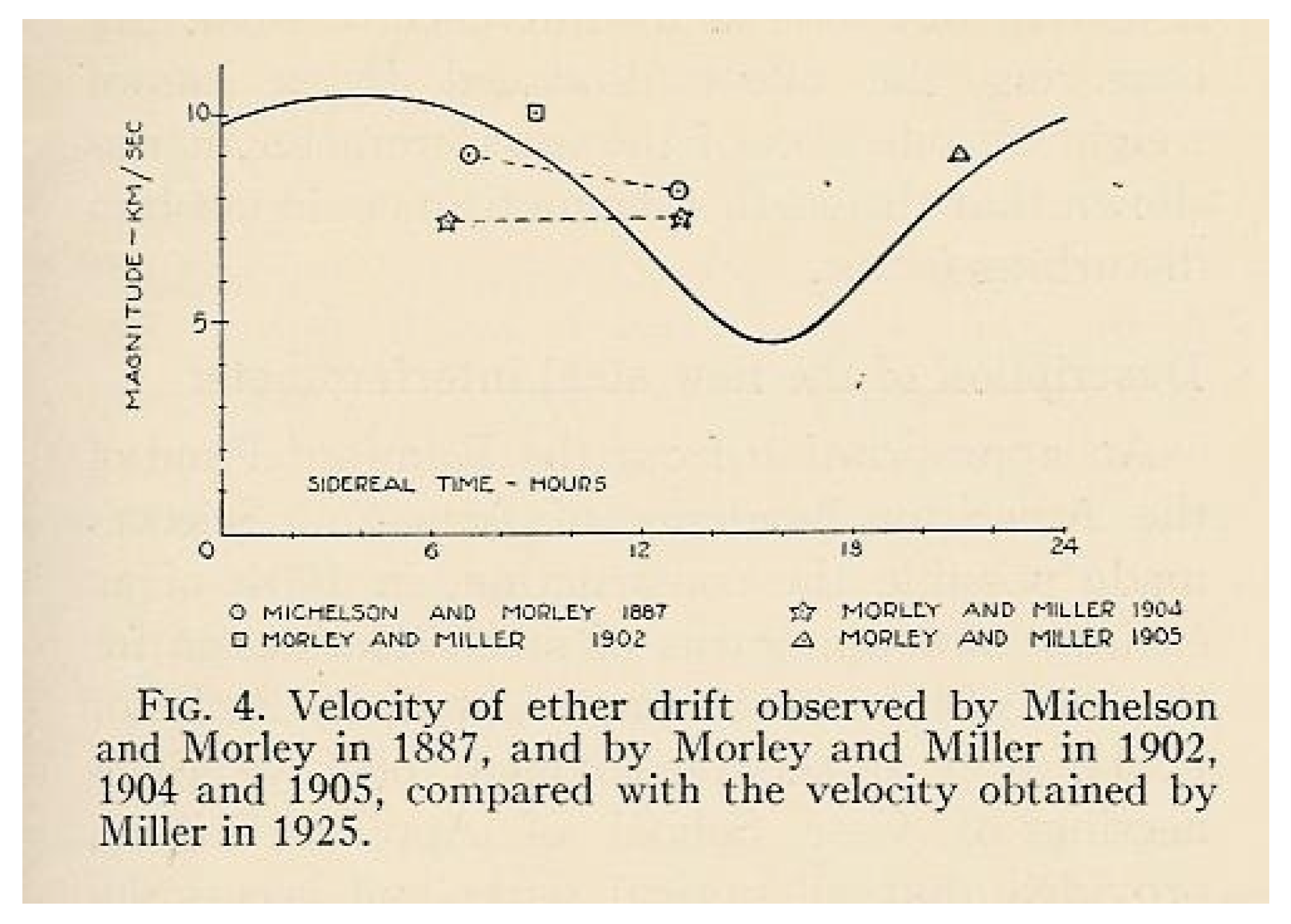
As an example, let us consider the second-harmonic amplitudes for the Michelson–Morley experiment; see

Table 1. The second-harmonic amplitudes for the six experimental sessions of the Michelson–Morley experiment. The table is taken from [37].

SESSION	${\mathit{A}}_2^{\mathbf{EXP}}$
8 July (noon)	$0.010\pm 0.005$
9 July (noon)	$0.015\pm 0.005$
11 July (noon)	$0.025\pm 0.005$
8 July (evening)	$0.014\pm 0.005$
9 July (evening)	$0.011\pm 0.005$
12 July (evening)	$0.024\pm 0.005$

. From these data, by computing the mean and variance, one finds $\langle A_2^{\mathrm{EXP}}\rangle \sim 0.016\pm 0.006$, so that by comparing with the classical prediction $A_2^{\mathrm{class}}=\frac{D}{\lambda }\frac{{\left(30\mathrm{km}/\mathrm{s}\right)}^2}{c^2}\sim 0.20$ and using Equation (25), we find an observable velocity $v_{\mathrm{obs}}\sim (8.4\pm 1.6)$ km/s, which is in good agreement with Miller’s analysis; see Figure 3. However, for air at atmospheric pressure where $ϵ\sim 2.8·{10}^{-4}$, the true kinematical value would instead be $\tilde{v}\sim (355\pm 70)$ km/s from Equation (45) or $\tilde{v}\sim (480\pm 95)$ km/s from Equation (46).

Let us then consider Miller’s very extensive observations. After the re-analysis of his work by the Shankland team [45], there is now the average second harmonic $\langle A_2^{\mathrm{EXP}}\rangle =0.044\pm 0.022$ for all epochs of the year (see Table III of [45]). By comparing this amplitude with the classical prediction for Miller’s apparatus $A_2^{\mathrm{class}}=\frac{D}{\lambda }\frac{{\left(30\mathrm{km}/\mathrm{s}\right)}^2}{c^2}\sim 0.56$, we find $v_{\mathrm{obs}}\sim (8.4\pm 2.2)$ km/s. However, the true kinematical velocity is instead $\tilde{v}\sim (355\pm 70)$ km/s according to Equation (45) or $\tilde{v}\sim (480\pm 95)$ km/s according to Equation (46).

Note the agreement of the two determinations obtained in very different conditions (the basement of the Cleveland laboratory or the top of Mount Wilson). This shows that the traditional interpretation [44,45] of the residuals as temperature differences in the optical paths is only acceptable provided that these temperature differences have a non-local origin. We will return to this point in Section 6.

There is no space for the details of all classical experiments. For that, we address the reader to our book [40], which also contains many historical notes and references to previous works. Here, we will limit ourselves to a brief description of Joos’ 1930 experiment [35] in Jena (sensitivity of about 1/3000 of a fringe), which is, by far, the most precise of the classical repetitions of the Michelson–Morley experiment and is considered the definitive disproof of Miller’s claims of a non-zero effect6.

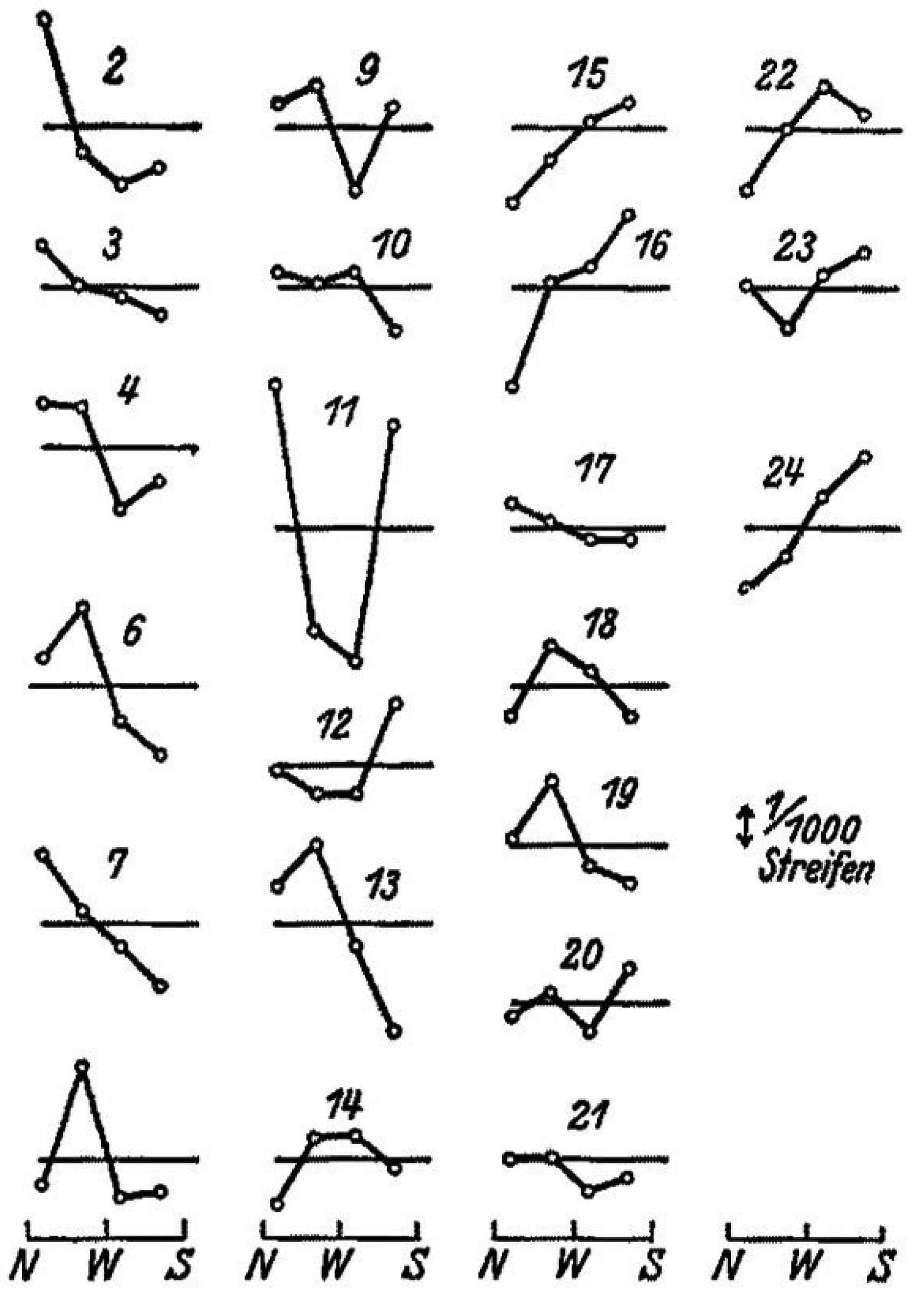
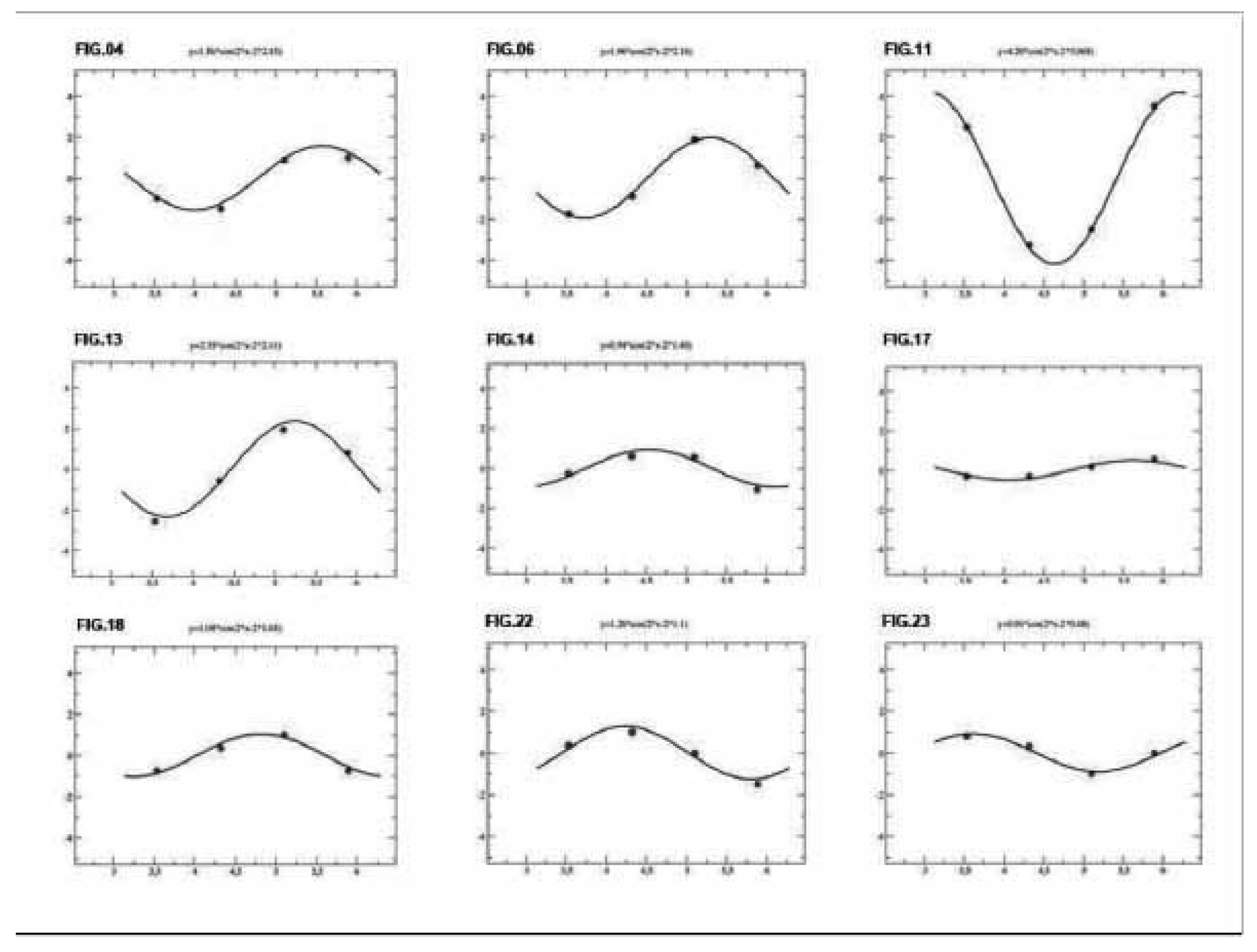
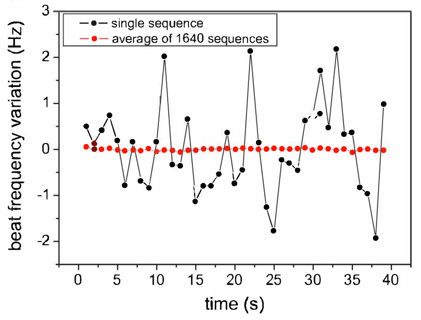
The data were taken at intervals of one hour during the sidereal day and recorded photographically with an automatic procedure; see Figure 4. From this picture, Joos adopted 1/1000 of a wavelength as the upper limit and deduced the bound of $v_{\mathrm{obs}}\lesssim 1.5$ km/s. To this end, he was comparing with the classical expectation that, for his apparatus, a velocity of 30 km/s should have produced a second-harmonic amplitude of 0.375 wavelengths. However, since it is apparent that some fringe displacements were certainly larger than 1/1000 of a wavelength, we performed second-harmonic fits for Joos’ data; see Figure 5. 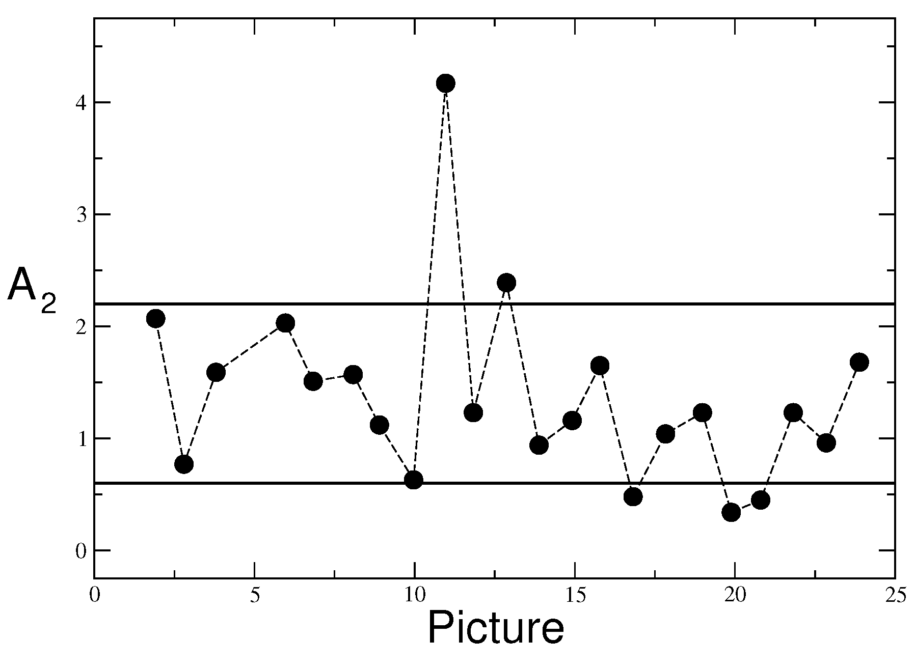The resulting amplitudes are reported in Figure 6.

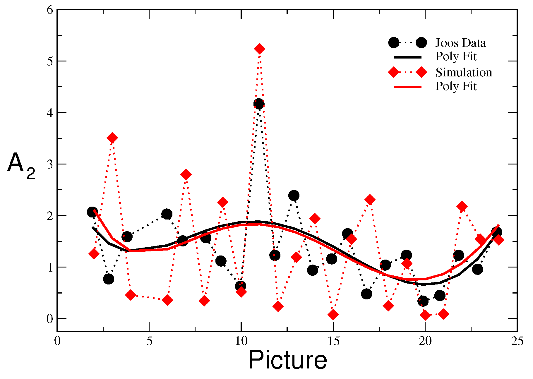
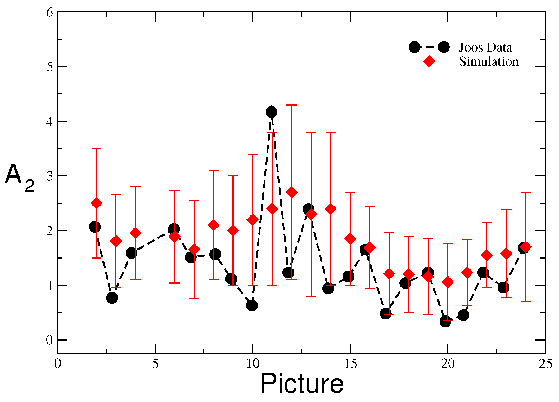
We note that the second-harmonic fit to the large fringe shifts in picture 11 has a very good chi-square, which is comparable and often better than those of other observations with smaller values; see Figure 5. Therefore, there is no reason to delete observation 11. Its amplitude, however, is more than ten times larger than the amplitudes from observations 20 and 21. This difference cannot be understood in a smooth model of the drift, where the projected velocity squared at the observation site can, at most, differ by a factor of two, as for the CMB motion at a typical Central European latitude, where ${\left(\tilde{v}\right)}_{\min }\sim 250$ km/s and ${\left(\tilde{v}\right)}_{\max }$ ∼ 370 km/s. To understand these characteristic fluctuations, we thus performed various numerical simulations of these amplitudes [37,40] in our stochastic model. To this end, Equations (36) and (37) were replaced in Equation (44), and the random velocity components were bounded by the kinematical parameters ${(V,\alpha ,\gamma )}_{\mathrm{CMB}}$, as explained in Section 4. Two simulations are shown in Figure 7 and Figure 8.

We would like to emphasize two aspects. First, Joos’ average amplitude $\langle A_2^{\mathrm{EXP}}\rangle =(1.4\pm 0.8)·{10}^{-3}$, when compared with the classical prediction for his interferometer $A_2^{\mathrm{class}}=\frac{D}{\lambda }\frac{{\left(30\mathrm{km}/\mathrm{s}\right)}^2}{c^2}\sim 0.375$, gives indeed an observable velocity $v_{\mathrm{obs}}\sim (1.8\pm 0.5)$ km/s, which is very close to the $1.5$ km/s value quoted by Joos. However, when comparing this with our prediction in the stochastic model in Equation (46), one would now find a true kinematical velocity of $\tilde{v}={305}_{-100}^{+85}$ km/s. Second, when fitting the smooth black curve of the Joos data in Figure 7 with Equations (29) and (30), one finds [37] a right ascension of $\alpha \left(\mathrm{fit}-\mathrm{Joos}\right)=(168\pm 30)$ degrees and an angular declination of $\gamma \left(\mathrm{fit}-\mathrm{Joos}\right)=(-13\pm 14)$ degrees, which are consistent with the present values of $\alpha \left(\mathrm{CMB}\right)\sim$ 168 degrees and $\gamma \left(\mathrm{CMB}\right)\sim -$7 degrees. This confirms that, when studied at different sidereal times, the measured amplitude can also provide precious information on the angular parameters.

Finally, all experiments are compared with our stochastic model in Equation (46) in

Table 2. The average second-harmonic amplitudes of classical ether-drift experiments. These were extracted from the original papers by averaging the amplitudes of the individual observations and assuming the direction of the local drift to be completely random (i.e., no vector averaging of different sessions). These experimental values were then compared with the full statistical average in Equation (46) for a projection of the velocity of 250 km/s $\le \tilde{v}\left(t\right)\le$ 370 km/s and refractivities of $ϵ=2.8·{10}^{-4}$ for air and $ϵ=3.3·{10}^{-5}$ for gaseous helium. The experimental value for the Morley–Miller experiment was taken from the observed velocities reported in Miller’s Figure 4 and, here, our Figure 3. The experimental value for the Michelson–Pease–Pearson experiment refers to the only known session for which the fringe shifts were reported explicitly [34] and where the optical path was still fifty-five feet. The symbol $\pm \dots .$ means that the experimental uncertainty cannot be determined from the available information.

Experiment	Gas	${\mathit{A}}_2^{\mathbf{EXP}}$	$\frac{2\mathit{D}}{\mathit{\lambda }}$	${\langle {\mathit{A}}_2\left(\mathit{t}\right)\rangle }_{\mathbf{stat}}$
Michelson (1881)	air	$(7.8 \pm \dots .)·{10}^{-3}$	$4·{10}^6$	$(0.7\pm 0.2)·{10}^{-3}$
Michelson–Morley (1887)	air	$(1.6\pm 0.6)·{10}^{-2}$	$4·{10}^7$	$(0.7\pm 0.2)·{10}^{-2}$
Morley–Miller (1902–1905)	air	$(4.0\pm 2.0)·{10}^{-2}$	$1.12·{10}^8$	$(2.0\pm 0.7)·{10}^{-2}$
Miller (1921–1926)	air	$(4.4\pm 2.2)·{10}^{-2}$	$1.12·{10}^8$	$(2.0\pm 0.7)·{10}^{-2}$
Tomaschek (1924)	air	$(1.0\pm 0.6)·{10}^{-2}$	$3·{10}^7$	$(0.5\pm 0.2)·{10}^{-2}$
Kennedy (1926)	helium	$<0.002$	$7·{10}^6$	$(1.4\pm 0.5)·{10}^{-4}$
Illingworth (1927)	helium	$(2.2\pm 1.7)·{10}^{-4}$	$7·{10}^6$	$(1.4\pm 0.5)·{10}^{-4}$
Piccard–Stahel (1928)	air	$(2.8\pm 1.5)·{10}^{-3}$	$1.28·{10}^7$	$(2.2\pm 0.8)·{10}^{-3}$
Mich.–Pease–Pearson (1929)	air	$(0.6 \pm \dots .)·{10}^{-2}$	$5.8·{10}^7$	$(1.0\pm 0.4)·{10}^{-2}$
Joos (1930)	helium	$(1.4\pm 0.8)·{10}^{-3}$	$7.5·{10}^7$	$(1.5\pm 0.6)·{10}^{-3}$

. Notice the substantial difference from the analogous summary in Table I of [45], where the authors compared with the classical relation $A_2^{\mathrm{class}}=\frac{D}{\lambda }\frac{{\left(30\mathrm{km}/\mathrm{s}\right)}^2}{c^2}$ and emphasized the much smaller magnitude of the experimental data. The opposite is the case here. In fact, our theoretical estimates are often smaller than the experimental results, indicating, most likely, the presence of systematic effects in the measurements. At the same time, however, by adopting Equation (46), the experiments in air give ${\tilde{v}}_{\mathrm{air}}\sim 418 \pm$ 62 km/s, and the two experiments in gaseous helium give ${\tilde{v}}_{\mathrm{helium}}\sim 323\pm 70$ km/s, with a global average of $\langle \tilde{v}\rangle \sim 376\pm 46$ km/s, which agrees well with the 370 km/s from the direct CMB observations. Moreover, from the most precise Piccard–Stahel and Joos experiments, we find two determinations, $\tilde{v}={360}_{-110}^{+85}$ km/s and $\tilde{v}={305}_{-100}^{+85}$ km/s, respectively, whose average of $\langle \tilde{v}\rangle \sim {332}_{-80}^{+60}$ km/s reproduces with high accuracy the projection of the CMB velocity at a typical Central European latitude7.

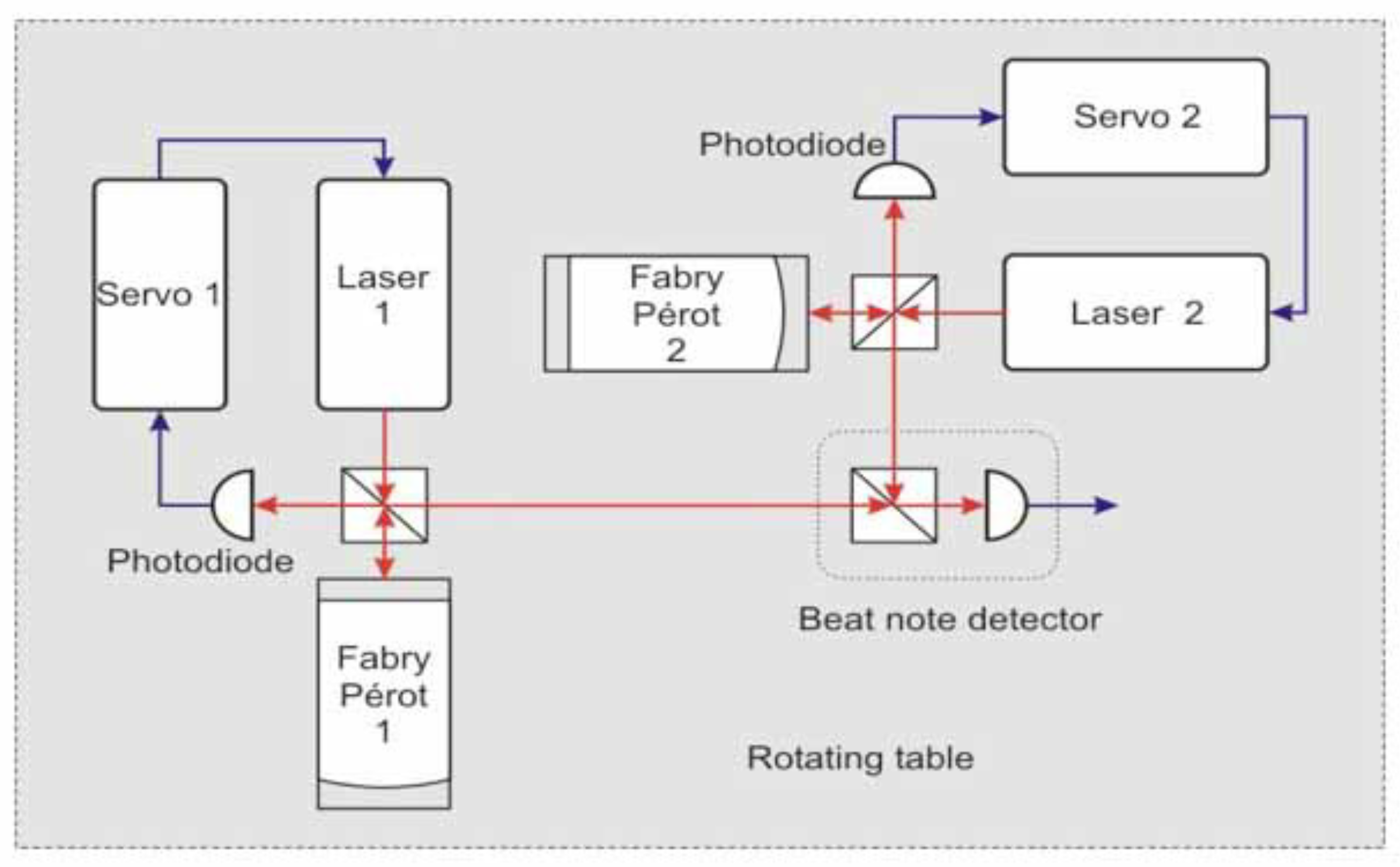
These non-trivial checks confirm the overall consistency of our picture with the classical experiments and should induce one to perform new and dedicated experiments where the optical resonators, which are coupled to lasers (see Figure 2), are filled with gaseous media. In this case, from Equation (7), one should compare the data with the prediction

$$\frac{\mathsf{\Delta }\nu \left(\theta \right)}{{\nu }_0}=\frac{\mathsf{\Delta }{\overline{c}}_{\theta }}{c}\sim ϵ\frac{v^2}{c^2}cos2(\theta -{\theta }_2)$$

(47)

However, precise measurements of the frequency shift in the gas mode are not so simple [70]. For this reason, it is unclear if there will be a definite improvement with respect to the classical experiments—in particular, with respect to Piccard–Stahel and Joos.

At present, a rough check of Equation (47) can, however, be obtained from the variations in the signal observed in the only modern experiment that was performed in these conditions: the 1963 experiment by Jaseja et al. [71] with He-Ne lasers. Actually, at that time, optical resonators were not yet used, and thus, they directly compared the frequencies of two orthogonal He-Ne lasers under 90-degree rotations of the apparatus. However, the light from the lasers emerged from a He-Ne gas mixture, and thus, the laser frequencies provided a measure of the two-way velocity of light in that environment. As a matter of fact, for a laser frequency of ${\nu }_0\sim 2.6·{10}^{14}$ Hz, after subtracting a large systematic effect of about 270 kHz due to magnetostriction, the residual variations of a few kHz are roughly consistent with the refractive index ${\mathcal{N}}_{\mathrm{He}-\mathrm{Ne}}\sim 1.00004$ and the typical change in the cosmic velocity of the Earth for the latitude of Boston. For more details, see the discussion given in [38,40].

6. Experiments in Gases vs. Vacuum and Solid Dielectrics

The results in Table 2 support the idea of a tiny $\frac{\mathsf{\Delta }{\overline{c}}_{\theta }}{c}$ at the level of ${10}^{-10}$ for the experiments in air and ${10}^{-11}$ for those in gaseous helium. Simple symmetry arguments suggest the relation $\frac{\mathsf{\Delta }{\overline{c}}_{\theta }}{c}\sim ({\mathcal{N}}_{\mathrm{gas}}-1)\frac{v^2}{c^2}$ so that, from the data, we find the typical velocity of $v\sim$ 300 km/s expected from our motion within the CMB. However, one could ask: Apart from symmetry arguments, what are the physical mechanisms producing this small observed anisotropy?

As a hint, we recall that Equation (8) was originally deduced in [18] as the most general angular dependence of the refractive index in the presence of convective currents of the gas molecules generated by an Earth velocity v. This idea of convection with respect to the container of the gas at rest in the laboratory leads to the reconsideration of the traditional explanation of the small residuals in terms of tiny temperature differences of a millikelvin or so [44,45]. The interesting aspect is that, aside from helping our intuition, this thermal interpretation will, in the end, be useful in analyzing the complementary region of the refractive index $\mathcal{N}$, which is very different from unity, as in solid dielectrics.

In principle, with angular differences $\mathsf{\Delta }{T}^{\mathrm{CMB}}\left(\theta \right)=\pm$ 3.36 mK in the background radiation Equation (2), temperature differences of a millikelvin could reflect the collisions of the gas molecules—at a mean velocity of 370 km/s—with the CMB photons. These collisions could bring the gas out of equilibrium and induce a temperature difference $\mathsf{\Delta }{T}^{\mathrm{gas}}\left(\theta \right)$ along the optical paths. In general, one expects $\mathsf{\Delta }{T}^{\mathrm{gas}}\left(\theta \right)\le \mathsf{\Delta }{T}^{\mathrm{CMB}}\left(\theta \right)$, and the two extreme cases $\mathsf{\Delta }{T}^{\mathrm{gas}}\left(\theta \right)=0$ and $\mathsf{\Delta }{T}^{\mathrm{gas}}\left(\theta \right)=\mathsf{\Delta }{T}^{\mathrm{CMB}}\left(\theta \right)$ correspond, respectively, to the limits of vanishing interactions or the complete thermalization of the two systems.

In view of the complexity of the calculation, we have not attempted a full microscopic derivation of the effect, but just limited ourselves to a much simpler thermodynamic analysis [39,40]. This just assumes the existence of some $\mathsf{\Delta }{T}^{\mathrm{gas}}\left(\theta \right)$ to derive a corresponding difference in the refractive index in the optical paths. Consistency with the idea of a non-local effect will then require the same average $\langle \mathsf{\Delta }{T}^{\mathrm{gas}}\left(\theta \right)\rangle$ from different experiments.

This type of analysis starts from the Lorentz–Lorentz equation:

$$\begin{array}{c}\hfill \frac{{\mathcal{N}}^2-1}{{\mathcal{N}}^2+2}=A_R\rho +B_R{\rho }^2\dots \end{array}$$

(48)

where $\rho$ is the molar density and $A_R=(4/3)\pi N_A\alpha$ is the product of the Avogadro number $N_A$ and the molecular polarizability $\alpha$ (see, e.g., [70]). The coefficient $B_R$ takes into account two-body interactions, which, for air and helium at atmospheric pressure, can be ignored. For $\mathcal{N}\sim 1$, we thus obtain the relation for the gas refractivity:

$$\begin{array}{c}\hfill ϵ=\mathcal{N}-1\sim \frac{3}{2}{A}_R\rho \end{array}$$

(49)

In the ideal-gas approximation, the molar density at STP (atmospheric pressure and $T=$ 273.15 K) has the value

$$\begin{array}{c}\hfill \rho \left(STP\right)=\frac{P}{RT}=\frac{101325}{\left(8.314\right)\left(273.15\right)}\mathrm{mol}·{\mathrm{m}}^{-3}\sim 4.46·{10}^{-5}\mathrm{mol}·{\mathrm{cm}}^{-3}\end{array}$$

(50)

As an example, for helium and a wavelength of $\lambda =$ 633 nm, where $\alpha \sim$ $0.52{\mathrm{mol}}^{-1}·{\mathrm{cm}}^3$ [70], this gives $ϵ\sim 3.5·{10}^{-5}$. Thus, in this simple approximation, where the temperature dependence of $ϵ$ is

$$\begin{array}{c}\hfill -\frac{\partial ϵ}{\partial T}\sim \frac{3}{2}{A}_R\frac{P}{R{T}^2}\sim \frac{ϵ\left(T\right)}{T}\end{array}$$

(51)

and from the relation ${\overline{c}}_{\gamma }\left(\theta \right)\equiv \frac{c}{\overline{\mathcal{N}}\left(\theta \right)}$, a difference $\mathsf{\Delta }{T}^{\mathrm{gas}}\left(\theta \right)$ is seen to induce a typical angular difference

$$\frac{|\mathsf{\Delta }{\overline{c}}_{\theta }|}{c}\sim |\overline{\mathcal{N}}\left(\theta \right)-\overline{\mathcal{N}}(\pi /2+\theta )|\sim \frac{ϵ\left(T\right)|\mathsf{\Delta }{T}^{\mathrm{gas}}\left(\theta \right)|}{T}$$

(52)

which should be visible in the fringe shifts with a second-harmonic amplitude of

$$A_2^{\exp }\sim \frac{2D}{\lambda }\frac{ϵ\left(T\right)|\mathsf{\Delta }{T}^{\mathrm{gas}}\left(\theta \right)|}{T}$$

(53)

For the average room temperature of $T\sim 288÷293$ K in the experiments, the values of $|\mathsf{\Delta }{T}^{\mathrm{gas}}\left(\theta \right)|$ are reported in

Table 3. The average second-harmonic amplitude observed in various classical ether-drift experiments and the resulting temperature differences (in mK) from Equation (53).

Experiment	Gas	${\mathit{A}}_2^{\mathbf{EXP}}$	$\frac{2\mathit{D}}{\mathit{\lambda }}$	$|\mathbf{\Delta }{\mathit{T}}^{\mathbf{gas}}\left(\mathit{\theta }\right)|$
Michelson–Morley (1887)	air	$(1.6\pm 0.6)·{10}^{-2}$	$4·{10}^7$	$0.40\pm 0.15$
Miller (1925–1926)	air	$(4.4\pm 2.2)·{10}^{-2}$	$1.12·{10}^8$	$0.39\pm 0.20$
Illingworth (1927)	helium	$(2.2\pm 1.7)·{10}^{-4}$	$7·{10}^6$	$0.29\pm 0.22$
Tomaschek (1924)	air	$(1.0\pm 0.6)·{10}^{-2}$	$3·{10}^7$	$0.33\pm 0.20$
Piccard–Stahel (1928)	air	$(2.8\pm 1.5)·{10}^{-3}$	$1.28·{10}^7$	$0.22\pm 0.12$
Joos (1930)	helium	$(1.4\pm 0.8)·{10}^{-3}$	$7.5·{10}^7$	$0.17\pm 0.10$

for the cases in which one can determine a meaningful experimental uncertainty.

The very good chi-square, 2.4/(6 − 1) = 0.48, shows that all experiments can become consistent with the same average value,

$$\langle \mathsf{\Delta }{T}^{\exp }\left(\theta \right)\rangle =(0.26\pm 0.06)\mathrm{mK}$$

(54)

so that the residuals observed in the old experiments could also be interpreted as thermal effects of non-local origin.

This previous analysis suggests two considerations. First, the old estimates of about 1 mK by Kennedy, Shankland, and Joos (see [44,45]) were slightly too large. Within our present view, this may indicate that the interactions of the gas molecules with the CMB photons are so weak that, on average, only less than 1/10 of $\mathsf{\Delta }{T}^{\mathrm{CMB}}\left(\theta \right)$ is transferred to the gas in the optical paths. Second, with the thermal mechanism discussed above, in Equation (18), one could replace ${ϵ}_{\mathrm{gas}}=({\mathcal{N}}_{\mathrm{gas}}-1)\equiv {ϵ}_{\mathrm{thermal}}+{ϵ}_v$ and re-write

$$\begin{array}{c}\hfill \frac{{\overline{\mathcal{N}}}_{\mathrm{gas}}\left(\theta \right)}{{\mathcal{N}}_{\mathrm{gas}}}\sim 1+({ϵ}_{\mathrm{thermal}}+{ϵ}_v){\beta }^2(1+{cos}^2\theta )\end{array}$$

(55)

where ${ϵ}_{\mathrm{thermal}}\equiv ({\mathcal{N}}_{\mathrm{gas}}-{\mathcal{N}}_v)$, ${ϵ}_v\equiv ({\mathcal{N}}_v-1)$. In this way, we have introduced an extremely small quantity ${ϵ}_v$, which, in principle, could still account for a difference between the velocity of light $c_{\gamma }\equiv c/{\mathcal{N}}_v$ as measured in a vacuum on the earth’s surface and the ideal parameter c of Lorentz transformations.

To roughly estimate a possible non-zero ${ϵ}_v$, let us first recall that, today, the (isotropic) speed of light in a vacuum is a reference standard with zero error—namely, $c_{\mathrm{ref}}=$ 299,792,458 m/s—and that the last precision measurements performed before fixing this reference value had an error of about 1 m/s at the 3-sigma level [72]. Therefore, assuming $|c - c_{\mathrm{ref}}| \lesssim$ 1 m/s, we would tentatively estimate ${ϵ}_v\lesssim {10}^{-9}$. As such, at room temperature and atmospheric pressure, where this ${ϵ}_v$ is numerically irrelevant, ${ϵ}_{\mathrm{thermal}}$ is practically the same as the refractive index considered so far, i.e., ${ϵ}_{\mathrm{air}}\sim 2.8·{10}^{-4}$ or ${ϵ}_{\mathrm{helium}}\sim 3.3·{10}^{-5}$. Nevertheless, Equation (55) is useful because, in the opposite limit of an extremely high vacuum, where, now, ${ϵ}_{\mathrm{thermal}}=0$, for ${ϵ}_v\ne 0$, we would predict the angular dependence

$$\begin{array}{c}\hfill \frac{{\overline{\mathcal{N}}}_v\left(\theta \right)}{{\mathcal{N}}_v}\sim 1+{ϵ}_v{\beta }^2(1+{cos}^2\theta )\end{array}$$

(56)

and an anisotropy of the two-way velocity of light in a vacuum:

$$\begin{array}{c}\hfill \frac{\mathsf{\Delta }{\overline{c}}_{\theta }}{c}{|}_{\mathrm{vacuum}}={\overline{\mathcal{N}}}_v\left(\theta \right)-{\overline{\mathcal{N}}}_v(\pi /2+\theta )\sim {ϵ}_v{\beta }^{2}cos2\theta \end{array}$$

(57)

Even more interestingly, the thermal argument is also useful for analyzing experiments in solid dielectrics, such as that originally performed by Shamir and Fox [43] in 1969. They were aware that the Michelson–Morley experiment did not yield a strictly zero result: “The non-zero result might have been real and due to the fact that the experiment was performed in air and not in vacuum” [43]. Therefore, within the traditional Lorentz-contraction interpretation of the experiment, with a refractive index $\mathcal{N}$ that is substantially above unity, one might expect a large $\frac{|\mathsf{\Delta }{\overline{c}}_{\theta }|}{c}\sim ({\mathcal{N}}^2-1){\beta }^2\sim {\beta }^2\sim {10}^{-6}$. This was the motivation for their experiment in perspex ($\mathcal{N}=1.5$). Since their measurements were orders of magnitude smaller, they concluded that the experimental basis of special relativity was strengthened.

However, with a thermal interpretation of the residuals in gaseous media, the two different behaviors can coexist. In fact, as anticipated in the introduction, in a system that is strongly bound as a solid, a small temperature gradient of a fraction of millikelvin would mainly dissipate through heat conduction without any particle motion or light anisotropy in the rest frame of the apparatus. On this basis, with a very precise experiment, a fundamental vacuum anisotropy, such as that in Equation (57), could also become visible in a solid dielectric.

To see how this works, let us first observe that, as in the gas case, for ${\mathcal{N}}_v\ne 1$, there will be a very tiny difference between the refractive index defined relative to the ideal vacuum value c and the refractive index relative to the physical isotropic vacuum value $c/{\mathcal{N}}_v$ measured on the Earth’s surface. The relative difference between these two definitions is proportional to ${ϵ}_v\lesssim {10}^{-9}$ and, for all practical purposes, can be ignored. More significantly, all materials would now exhibit the same background vacuum anisotropy proportional to ${ϵ}_v{\beta }^2$ in Equation (57). To this end, let us first replace the average isotropic value

$$\frac{c}{{\mathcal{N}}_{\mathrm{solid}}}\to \frac{c}{{\mathcal{N}}_v{\mathcal{N}}_{\mathrm{solid}}}$$

(58)

and then use Equation (56) to replace ${\mathcal{N}}_v$ in the denominator with ${\overline{\mathcal{N}}}_v\left(\theta \right)$. This is equivalent to defining a $\theta$—dependent refractive index for the solid dielectric

$$\begin{array}{c}\hfill \frac{{\overline{\mathcal{N}}}_{\mathrm{solid}}\left(\theta \right)}{{\mathcal{N}}_{\mathrm{solid}}}\sim 1+{ϵ}_v{\beta }^2(1+{cos}^2\theta )\end{array}$$

(59)

so that

$${\left[{\overline{c}}_{\gamma }\left(\theta \right)\right]}_{\mathrm{solid}}=\frac{c}{{\overline{\mathcal{N}}}_{\mathrm{solid}}\left(\theta \right)}=\frac{c}{{\mathcal{N}}_{\mathrm{solid}}}\left[1-{ϵ}_v{\beta }^2(1+{cos}^2\theta )\right]$$

(60)

with an anisotropy

$$\frac{{\left[\mathsf{\Delta }{\overline{c}}_{\theta }\right]}_{\mathrm{solid}}}{\left[c/{\mathcal{N}}_{\mathrm{solid}}\right]}\sim {ϵ}_v{\beta }^{2}cos2\theta$$

(61)

In this way, a genuine vacuum effect, such as that in Equation (57), if present, could also be detected with a very precise experiment in a solid dielectric. It is then important to understand the magnitude ${ϵ}_v\lesssim {10}^{-9}$ suggested by the last precision measurements of about thirty years ago [72]. Is it just accidental, or does it express a fundamental property of light on the Earth’s surface? In the latter case, with ${ϵ}_v\sim {10}^{-9}\ne 0$ in Equations (57) and (61), a typical ${10}^{-15}$ signal should then show up. Let us therefore compare this with present experiments, starting from those with vacuum optical resonators.

7. Modern Experiments with Optical Resonators

7.1. Basic Aspects of Present Experiments in Vacuum

As anticipated, the Pound–Drever–Hall system [53,54] shown in Figure 2 was crucial for precision tests of relativity. The first application dates back to Brillet and Hall in 1979 [73]. They were comparing the frequency of a CH${}_4$ reference laser (fixed in the laboratory) with the frequency of a cavity-stabilized He-Ne laser placed on a rotating table. Since the stabilizing optical cavity was placed inside a vacuum envelope, the measured shift $\mathsf{\Delta }\nu \left(\theta \right)$ gave a measure of the anisotropy of the velocity of light in vacuum.

In the last forty years, substantial improvements have been introduced into the experiments. However, the assumptions behind the analysis of the data are basically unchanged, and any physical signal is assumed to depend deterministically on the velocity of the Earth with respect to some fixed preferred frame. As emphasized in the previous chapters, the macroscopic motion of the Earth (i.e., on a cosmic scale) could instead affect the microscopic propagation of light in an optical cavity in some complicated, indirect way, and a genuine signal could easily be misinterpreted as a spurious effect. For this reason, first of all, we will try to understand the magnitude of the instantaneous signal with vacuum cavities and then compare the data with numerical simulations performed within the same model as that adopted for the classical experiments.

To understand the magnitude of the signal, we have compared with Figure 9a of [47] and Figure 4 [51]. These give the idea of a very irregular $\mathsf{\Delta }\nu$ with a typical magnitude in the range of $\pm 1$ Hz; see our Figure 9. For the adopted reference frequency ${\nu }_0=2.8·{10}^{14}$ Hz, this is the anticipated ${10}^{-15}$ fractional level. The same value was obtained from [48]. Actually, in this other article, the instantaneous signal is not shown explicitly, but it can be deduced from the typical variation over a characteristic time of 1 ÷ 2 s. For an irregular signal, in fact, this variation gives the magnitude of the signal itself, and its value is, again, ${10}^{-15}$.

After having obtained these first indications, we tried to understand the meaning of this irregular signal. Namely, is it just spurious noise (e.g., thermal noise [74]), or could it represent a genuine signal? As a check, we then compared with other two experiments, those of [46,50], where the optical cavities were made of different materials and were operating at a cryogenic temperature. Again, the same ${10}^{-15}$ level was found. Since it is extremely unlikely that spurious effects remain the same for experiments operating in such different conditions, it is natural to explore the possibility that this ${10}^{-15}$ signal admits a physical interpretation.

Therefore, applying to the physical vacuum the same model that was used successfully for the classical experiments, we will tentatively express this observed fractional shift in terms of a cosmic Earth velocity and of a refractive index ${\mathcal{N}}_v$ as

$${\left|\frac{\mathsf{\Delta }\nu \left(\theta \right)}{{\nu }_0}\right|}_{\exp }={\left|\frac{\mathsf{\Delta }{\overline{c}}_{\theta }}{c}\right|}_{\exp }\sim ({\mathcal{N}}_v-1)(v^2/c^2)\sim \mathcal{O}\left({10}^{-15}\right)$$

(62)

For $v\sim$ 300 km/s, this supports our previous idea of a tiny refractivity of ${ϵ}_v=({\mathcal{N}}_v-1)\sim {10}^{-9}$ for the physical vacuum established in an apparatus placed on the Earth’s surface. Therefore, it is now the time to recall the scenario of [52], which could indeed explain this result.

7.2. A 10⁻⁹ Refractivity for the Vacuum on the Earth’s Surface

The idea of a non-zero vacuum refractivity may have different motivations. The perspective of [52] was inspired by the so-called emergent gravity approach [75,76,77,78,79,80,81], where the introduction of a non-trivial metric field $g_{\mu \nu }\left(x\right)$ is considered in analogy with the hydrodynamic limit of many condensed-matter systems. This emergent interpretation is made manifest in a parametric dependence of the metric on some auxiliary, gravity-inducing fields $s_k\left(x\right)$, i.e., $g_{\mu \nu }\left(x\right)=g_{\mu \nu }\left[s_k\left(x\right)\right]$. As in the pioneering Yilmaz derivation based on the static Newtonian potential [82,83], the Einstein equations for the metric would then follow from the equations of motion for the $s_k$s in flat space after introducing a suitable stress tensor for these auxiliary fields. In this way, one could (partially) fill the conceptual gap with classical General Relativity.

An interesting consequence derives from the boundary condition $g_{\mu \nu }[s_k=0]={\eta }_{\mu \nu }$. In fact, if the $s_k$s are understood as excitations of the physical vacuum, which therefore vanish identically in its equilibrium state, one could easily understand [77] why the energy of the unperturbed vacuum plays no role. This perspective of a non-gravitating vacuum energy [77] provides, perhaps, the most intuitive solution of the so-called cosmological-constant problem that is usually mentioned in connection with the quantum vacuum. In this sense, with this type of approach, one takes Feynman’s words seriously: “The first thing we should understand is how to formulate gravity so that it doesn’t interact with the vacuum energy” [84].

Another interesting aspect of this approach is that, even without knowing the underlying $s_k$s, in the simplest case of a static metric, all dynamical effects are equivalent to two basic ingredients: (i) local modifications of the physical clocks and rods and (ii) local modifications of the velocity of light. Therefore, with this interpretation of the observed curvature, one could try to test the fundamental assumption of General Relativity that, in the presence of gravity, the velocity of light in vacuum $c_{\gamma }$ is still a universal constant—namely, it remains the same basic parameter c of Lorentz transformations. Notice that, here, we are not considering the so-called coordinate-dependent speed of light. Rather, we are focused on the true, physical $c_{\gamma }$, as obtained from experimental measurements in vacuum optical cavities placed on the Earth’s surface. Thus, in principle, a precise measurement that establishes that $c_{\gamma }\ne c$ could give information on the fundamental mechanisms at the base of the gravitational interaction.

For the various aspects of space-time measurements, a very clear reference is Cook’s article, “Physical time and physical space in general relativity” [85]. There, the appropriate units of time and length ($d\tau$ and $dl$, respectively) are defined to ensure that all observers measure the same universal speed of light (“Einstein postulate”). For a static metric, these definitions are $d{\tau }^2=g_{00}d{t}^2$ and $d{l}^2=g_{ij}d{x}^{i}d{x}^j$. Thus, in General Relativity, the condition $d{s}^2=0$, which governs the propagation of light, can be expressed formally as

$$d{s}^2=c^{2}d{\tau }^2-d{l}^2=0$$

(63)

and, by construction, always gives the same speed $dl/d\tau =c$.

However, if the physical units were instead $d\widehat{\tau }$ and $d\widehat{l}$ with, say, $d\tau =qd\widehat{\tau }$ and $dl=pd\widehat{l}$, the same condition

$$d{s}^2=c^2{q}^{2}d{\widehat{\tau }}^2-p^{2}d{\widehat{l}}^2=0$$

(64)

would now be interpreted differently as

$$c_{\gamma }=\frac{d\widehat{l}}{d\widehat{\tau }}=c\frac{q}{p}\equiv \frac{c}{{\mathcal{N}}_v}$$

(65)

The possibility of different units is thus a simple motivation for a vacuum refractive index of ${\mathcal{N}}_v\ne 1$.

To fix the ideas, we will start from the unambiguous point of view of special relativity: The right space-time units are those for which the speed of light in the vacuum $c_{\gamma }$, when measured in an inertial frame, coincides with the basic parameter c of Lorentz transformations. However, inertial frames are just an idealization. Therefore, the physical realization is to assume standards of distance and time that can change locally, but such that the identification $c_{\gamma }=c$ holds in the asymptotic condition, which is as close as possible to an inertial frame. This asymptotic condition corresponds to measure $c_{\gamma }$ in a freely falling frame8 and is crucial for an operational definition of the otherwise unknown quantity c.

With this premise, an observer $S^{\prime }$ placed on the Earth’s surface can still describe light propagation in different ways. We address the reader to [52], where these aspects were originally discussed, and to [39,40] for further refinements. The whole idea, however, is simple and can be reduced to Figure 10. An observer $S^{\prime }$ placed on the Earth’s surface is in free-fall with respect to all masses in the Universe, but not with respect to the gravitational field of the Earth. Its effect can be schematically represented by means of a heavy mass M carried on board of an elevator.

The two situations in panels (a) and (b) of Figure 10 are physically distinct, but in General Relativity, it is assumed that both observers will measure the same c of Lorentz transformations. A non-zero vacuum refractivity for system (b) can thus be expressed as

$${ϵ}_v={\mathcal{N}}_v-1\sim \frac{z}{2}\left(\frac{2\left|\delta U\right|}{c^2}\right)$$

(66)

where $\delta U$ is the extra Newtonian potential produced by the heavy mass M at the experimental setup. In General Relativity, one assumes $z=0$, while the two non-zero values ($z=$ 1 or 2) account for the two alternatives traditionally reported in the literature for the effective refractive index in a gravitational potential (see the discussion in [39,40] and, in particular, Broekaert’s footnote${}^3$ [86]). In our case, by introducing the Newton constant, the radius R, and the mass M of the Earth so that $\delta U=\frac{G_{N}M}{R}$, we find

$${ϵ}_v\sim \frac{z}{2}1.4·{10}^{-9}$$

(67)

We emphasize that, regardless of whether $z=$ 1 or 2, the velocity of light in a vacuum cavity on the Earth’s surface (panel (b) in our Figure 10) could differ at the level of ${10}^{-9}$ from the ideal value c, which is operationally defined with the same apparatus in a truely freely falling frame (panel (b) in our Figure 10). As discussed at the end of Section 6, this ${ϵ}_v\sim {10}^{-9}$ was suggested by the last precise measurements of the velocity of light and, by comparing with Equation (62), could now provide a physical argument for seriously considering the presently observed ${10}^{-15}$ fractional frequency shift of two vacuum optical resonators. Let us therefore take a closer look at the present experiments.

7.3. A Closer Look at Experiments and Numerical Simulations of the Signal

Most recent ether-drift experiments measure the frequency shift $\mathsf{\Delta }\nu$ of two rotating optical resonators. To this end, let us re-write Equation (26) as

$$\frac{\mathsf{\Delta }\nu \left(t\right)}{{\nu }_0}=\frac{\mathsf{\Delta }{\overline{c}}_{\theta }\left(t\right)}{c}\sim ϵ\frac{v^2\left(t\right)}{c^2}cos2({\omega }_{\mathrm{rot}}t-{\theta }_2\left(t\right))$$

(68)

where ${\omega }_{\mathrm{rot}}$ is the rotation frequency of the apparatus. Therefore, one finds

$$\frac{\mathsf{\Delta }\nu \left(t\right)}{{\nu }_0}\sim 2S\left(t\right)sin2{\omega }_{\mathrm{rot}}t+2C\left(t\right)cos2{\omega }_{\mathrm{rot}}t$$

(69)

where $C\left(t\right)$ and $S\left(t\right)$ are given in Equations (28) for $ϵ={ϵ}_v$,

$$2C\left(t\right)={ϵ}_v\frac{v_x^2\left(t\right)-v_y^2\left(t\right)}{c^2}2S\left(t\right)={ϵ}_v\frac{2v_x\left(t\right)v_y\left(t\right)}{c^2}$$

(70)

and $v_x\left(t\right)=v\left(t\right)cos{\theta }_2\left(t\right)$, $v_y\left(t\right)=v\left(t\right)sin{\theta }_2\left(t\right)$. For a non-rotating apparatus, such as that in Figure 9, the fractional frequency shift is thus simply $2C\left(t\right)$.

The present analysis of the data is the following. For short-term observations of a few days, the frequency shifts measured upon rotation of the apparatus are used to extract the instantaneous 2C(t) and 2S(t) through Equation (69). These data are then compared with the parameterizations in Equations (33) and (34) to fit the $C_k$ and $S_k$ Fourier coefficients. From very extensive observations, the present values of these coefficients are at the level of ${10}^{-18}÷{10}^{-19}$, i.e., about 1000 times smaller than the typical ${10}^{-15}$ instantaneous signal.

By recalling our discussion at the beginning of Section 5, this is exactly the same strategy that was traditionally adopted for the fringe shifts in the old experiments and that cannot be maintained with a genuine irregular signal. In fact, within our isotropic model (see Equations (41) and (42)), one would find ${\langle C\left(t\right)\rangle }_{\mathrm{stat}}=0$ and ${\langle S\left(t\right)\rangle }_{\mathrm{stat}}=0$ at any time t and mean values of ${\left(C_k\right)}^{\mathrm{avg}}=0$, ${\left(S_k\right)}^{\mathrm{avg}}=0$ for all Fourier coefficients. Therefore, with an irregular but genuine signal, a different type of analysis is needed.

To compare with the data, we performed numerical simulations in our isotropic stochastic model of Section 4 with ${ϵ}_v$, as in Equation (67). As a first illustration, we show in Figure 11 two sequences of the instantaneous values for 2C(t) and 2S(t). The two sets belong to the same random sequence and refer to two sidereal times that differ by 6 h. The set ${(V,\alpha ,\gamma )}_{\mathrm{CMB}}$ was adopted to control the boundaries of the stochastic velocity components through Equations (29), (30), and (40). The value of $\varphi =52$ degrees was also fixed to reproduce the average latitude of the laboratories in Berlin and Düsseldorf. For a laser frequency of $2.8·{10}^{14}$ Hz [51], the interval $\pm 3.5·{10}^{-15}$ of these dimensionless amplitudes corresponds to a random instantaneous frequency shift $\mathsf{\Delta }\nu$ in the typical range of $\pm 1$ Hz, as in our Figure 9.

For a more quantitative analysis, we considered the result of [51] for the average variation in the frequency shift over 1 s; see their Figure 3, bottom part. This corresponds to a Root Square of the Allan Variance (RAV) of about $0.24$ Hz, or $8.5·{10}^{-16}$ at a fractional level. In general, the RAV describes the time dependence of an arbitrary function $f=f\left(t\right)$, which can be sampled over time intervals of length $\tau$. By defining

$$\overline{f}(t_i;\tau )=\frac{1}{\tau }{\int }_{t_i}^{t_i+\tau }dtf\left(t\right)\equiv {\overline{f}}_i$$

(71)

one generates a $\tau$-dependent distribution of ${\overline{f}}_i$ values. In a large time interval $\mathsf{\Lambda }=M\tau$, the RAV is then defined as

$${\sigma }_A(f,\tau )=\sqrt{{\sigma }_A^2(f,\tau )}$$

(72)

where

$${\sigma }_A^2(f,\tau )=\frac{1}{2(M-1)}\sum _{i=1}^{M-1}{\left({\overline{f}}_i-{\overline{f}}_{i+1}\right)}^2$$

(73)

The integration time $\tau$ is given in s, and the factor of 2 is introduced to obtain the same standard variance for uncorrelated data as for a white-noise signal with a uniform spectral amplitude at all frequencies.

To understand the characteristics of our signal, we thus simulated one-day measurements of $2C\left(t\right)$ and $2S\left(t\right)$ at steps of 1 s. The RAV and the standard variance agreed with a good accuracy, so the signal of our isotropic stochastic model could be approximated as a pure white noise. From these simulations of one-day measurements ($z=$ 1 or 2), we obtained mean values of ${\langle 2C\rangle }_{\mathrm{day}}=-1.6·(z/2)·{10}^{-18}$ and ${\langle 2S\rangle }_{\mathrm{day}}=4.3·(z/2)·{10}^{-18}$ and variances of

$${\left[{\sigma }_A(2C,1)\right]}_{\mathrm{simul}}=\frac{z}{2}(8.7\pm 0.8)·{10}^{-16}$$

(74)

$${\left[{\sigma }_A(2S,1)\right]}_{\mathrm{simul}}=\frac{z}{2}(9.6\pm 0.9)·{10}^{-16}$$

(75)

Here, the ± uncertainties reflect the observed variations due to the truncation of the Fourier modes in Equations (36) and (37) and to the dependence on the random sequence. From Equation (69), by quadratically combining these two sigmas, we estimate

$${\left[{\sigma }_A(\frac{\mathsf{\Delta }\nu }{{\nu }_0},1)\right]}_{\mathrm{simul}}\sim \sqrt{\frac{1}{2}{\sigma }_A^2{[2C,1]}_{\mathrm{simul}}+\frac{1}{2}{\sigma }_A^2{[2S,1]}_{\mathrm{simul}}}\sim \frac{z}{2}(9.2 \pm 0.9)·{10}^{-16}$$

(76)

so that, for a laser frequency of ${\nu }_0=2.8·{10}^{14}$ Hz [51], we would predict an average RAV of

$${\left[{\sigma }_A(\mathsf{\Delta }\nu ,1)\right]}_{\mathrm{simul}}\sim \frac{z}{2}(0.26 \pm 0.03)\mathrm{Hz}$$

(77)

of the frequency shift at 1 s. This estimate should be compared with the aforementioned experimental value of

$${\left[{\sigma }_A(\mathsf{\Delta }\nu ,1)\right]}_{\exp }\sim 0.24\mathrm{Hz}$$

(78)

reported in [51]. The good agreement with our simulated value indicates that, at least for an integration time of 1 s, the correction to our model should be negligible. In addition, the data favor $z=2$, which is the only free parameter of our scheme.

Our model, however, makes another definite prediction: During the day, there should be characteristic modulations that reflect the periodic variations of $\tilde{v}\left(t\right)$ Equation (30) in the plane of the interferometer. For $z=2$ and the typical Central European value of $\tilde{v}\left(t\right)=(250÷370)$ km/s, taking into account the uncertainties in the simulations, from bins of data centered around the various times t, the RAV at 1 s explores the range

$$5·{10}^{-16}\lesssim {\left[{\sigma }_A(\frac{\mathsf{\Delta }\nu }{{\nu }_0},1)\right]}_t\lesssim 12·{10}^{-16}$$

(79)

This range was obtained with our numerical simulation, but can be approximated as

$${\left[{\sigma }_A(\frac{\mathsf{\Delta }\nu }{{\nu }_0},1)\right]}_t\sim 8.4·{10}^{-16}{\left(\frac{\tilde{v}\left(t\right)}{315\mathrm{km}/\mathrm{s}}\right)}^2$$

(80)

where $\tilde{v}\left(t\right)$ is defined in Equation (30).

Detecting these periodic variations would therefore give the cleanest test of our picture, provided that these variations are not obscured by spurious effects. The simplest strategy for a comparison is to determine—from the spectral amplitude of the experimental signal—the frequency ${\omega }_0$ beyond which the spectral amplitude $\sqrt{S\left(\omega \right)}$ becomes flat. Thus, by defining ${\tau }_0\sim {\omega }_0^{-1}$, for integration times of $\tau \lesssim {\tau }_0$, the RAV is dominated by the pure white-noise component of the signal. Then, since, typically, ${\tau }_0\sim$ 1 s, by measuring the experimental RAV at ${\tau }_0$ in different hours of the day, one can directly compare with Equation (79)9.

For a more refined comparison, one could try to generate a colored signal that, as in the real experimental situation, contains various branches (white noise, pink noise, random walk, etc.), and one could try to directly estimate the modifications of our basic white-noise component at the various $\tau$s. Since these modifications depend on the particular experiment, we decided to consider [25]. This was a high-precision cryogenic experiment with microwaves of 12.97 GHz, where almost all electromagnetic energy propagated in a medium (sapphire) with a refractive index of about 3 (at microwave frequencies). Therefore, an analysis of this experiment will also check our Equation (61), implying that, with very precise measurements, a fundamental ${10}^{-15}$ vacuum signal such as that in (57) should also show up in a solid dielectric.

In Figure 3c of [25], the spectral amplitude of this particular apparatus is seen to become flat at frequencies of $\omega \ge 0.5$ Hz, indicating the estimate of the order of magnitude of ${\tau }_0\sim$ 1 s. In collaboration with Dr. Giancarlo Cella of the VIRGO Collaboration, these data for the spectral amplitude were then fitted to an analytic power-law form to describe the lower-frequency part at 0.001 Hz $\le \omega \le 0.5$ Hz. This fitted spectrum was then used to generate a signal with a Fourier transform. Finally, very long sequences of this signal were stored to produce a “colored” version of our basic white-noise signal. The details of this analysis will be published elsewhere [87].

Here, we will limit ourselves to reporting the results of a first set of simulations in intervals of 2000 s. To obtain a qualitative impression of the effect, we show in Figure 12 a sequence of our basic white-noise signal and a sequence of its colored version. After averaging over many 2000-s sequences of this type, the corresponding RAVs for the two signals are shown in Figure 13. The experimental RAV extracted from Figure 3b of [25] is also reported (for the non-rotating setup). At this stage, the agreement of our simulated, colored signal with the experimental data only remains satisfactory up $\tau =$ 50 s. Reproducing the signal at larger $\tau$s will require further efforts, but this is not relevant here, as our scope is just to understand the modifications of our stochastic signal near the 1-s scale.

From Figure 13, we find that, at the value of interest $\tau =$ 1 s, our predicted white-noise signal $(7.1\pm 0.3)·{10}^{-16}$ is changed by about $+15\%$ when comparing with our simulated colored value $(8.2\pm 0.3)·{10}^{-16}$ or by about $+20\%$ when comparing with the experimental value of about $8.5·{10}^{-16}$. Thus, if present in the experimental data the periodic variations of a factor of 2, as in Equation (79), should remain visible, at least with the systematics at the level of [25].

At the same time, this $8.5·{10}^{-16}$ that was obtained in [25] for the experimental RAV at 1 s is the same $8.5·{10}^{-16}$ that we extracted from the value of ${\sigma }_A{(\mathsf{\Delta }\nu ,1)}_{\exp }\sim$ 0.24 Hz from [51] after normalizing to the laser frequency of ${\nu }_0=2.8·{10}^{14}$ Hz. Therefore, this beautiful agreement between [51] (a vacuum experiment at room temperature) and [25] (a cryogenic experiment in a solid dielectric), while confirming our predictions in Equations (57) and (61) of a fundamental ${10}^{-15}$ signal, indicates that periodic variations such as those in Equation (79) should also remain visible with the apparatus of [51].

8. Summary and Conclusions

Due to the present interpretation of the dominant dipole anisotropy of the Cosmic Microwave Background as a Doppler effect, one may wonder about the reference system in which this dipole exactly vanishes. Since the observed motion is, to a good approximation, the combination of peculiar motions and reflects local inhomogeneities, one could naturally consider the idea of a global frame of rest associated with the Universe as a whole that could characterize the form of relativity physically realized in nature. The isotropy of the CMB could then just indicate the existence of this fundamental system $\mathsf{\Sigma }$, which we could conventionally decide to call “ether”, but the cosmic radiation itself would not coincide with this type of ether. Due to the fundamental group properties of Lorentz transformations, two observers individually moving with respect to $\mathsf{\Sigma }$ would still be connected by the standard relativistic composition rule of velocities. However, ultimate implications could be far reaching, even when considering just the interpretation of non-locality in the quantum theory.

Since the answer cannot be found on purely theoretical grounds, physical interpretation is traditionally postponed to the detection of some dragging of light in the Earth frame—namely, to measuring a small angular dependence $\frac{\mathsf{\Delta }{\overline{c}}_{\theta }}{c}$ of the two-way velocity of light in the laboratory and trying to correlate the measurements with the direct CMB observations with satellites in space. The present view is that no such meaningful correlations have ever been observed, and all data collected so far (from Michelson–Morley to the modern experiments with optical resonators) are just considered typical instrumental effects in measurements with better and better systematics.

However, if the velocity of light in the interferometers is not the same parameter “c” of Lorentz transformations, nothing would prevent a non-zero dragging. For instance, in experiments in gaseous media with a refractive index of $\mathcal{N}=1+ϵ$, the small fraction of refracted light could keep track of the velocity of matter with respect to the hypothetical $\mathsf{\Sigma }$ and produce a direction-dependent refractive index. Then, from symmetry arguments that are valid in the $ϵ\to 0$ limit, one would expect $\frac{|\mathsf{\Delta }{\overline{c}}_{\theta }|}{c}\sim ϵ(v^2/c^2)$, which is much smaller than the classical expectation of $\frac{|\mathsf{\Delta }{\overline{c}}_{\theta }{|}_{\mathrm{class}}}{c}\sim (v^2/2c^2)$. For $v\sim$ 300 km/s, and by inserting the appropriate refractive index, i.e., $ϵ\sim 2.8·{10}^{-4}$ for air and $ϵ\sim 3.3·{10}^{-5}$ for gaseous helium, this reproduces the observed order of magnitude: $\frac{|\mathsf{\Delta }{\overline{c}}_{\theta }|}{c}\sim {10}^{-10}$ and $\frac{|\mathsf{\Delta }{\overline{c}}_{\theta }|}{c}\sim {10}^{-11}$, respectively.

In addition, aside from being much smaller than classically expected, observable effects could have an irregular nature. This means that the projection of the global velocity field at the site of the experiment, say ${\tilde{v}}_{\mu }\left(t\right)$, could differ non-trivially from the local field $v_{\mu }\left(t\right)$, which determines the instantaneous direction and magnitude of the drift in the plane of the interferometer. As a definite model, to relate $v_{\mu }\left(t\right)$ and ${\tilde{v}}_{\mu }\left(t\right)$, we followed the physical analogy with a turbulent fluid—in particular, with the form of turbulence that, at small scales, becomes statistically homogeneous and isotropic. To this end, the local $v_{\mu }\left(t\right)$ was expanded in a large number of Fourier components that varied randomly within boundaries that depended on the smooth ${\tilde{v}}_{\mu }\left(t\right)$ determined by the average motion of the Earth. In this model, at the small scale of the experiment, statistical averages of vector quantities vanish identically. Therefore, one should analyze the data for $\frac{\mathsf{\Delta }{\overline{c}}_{\theta }\left(t\right)}{c}$ in phase ${\theta }_2\left(t\right)$ and amplitude $A_2\left(t\right)$, which give, respectively, the direction and magnitude of the local drift, and concentrate on the latter, which, being positive definite, remains non-zero under any averaging procedure. Then, even discarding ${\theta }_2\left(t\right)$, the average value and the time modulations of the statistical average ${\langle A_2\left(t\right)\rangle }_{\mathrm{stat}}$ would be sufficient to correlate a genuine signal with the corresponding cosmic motion.

As proof, we report some remarkable correlations found in the old experiments:

(a) By fitting the smooth polynomial interpolation of the irregular Joos second-harmonic amplitudes in our Figure 7 with Equations (29) and (30), one finds [37] a right ascension of $\alpha \left(\mathrm{fit}-\mathrm{Joos}\right)=(168\pm 30)$ degrees and an angular declination of $\gamma \left(\mathrm{fit}-\mathrm{Joos}\right)=(-13\pm 14)$ degrees, which are consistent with the present values of $\alpha \left(\mathrm{CMB}\right)\sim$ 168 degrees and $\gamma \left(\mathrm{CMB}\right)\sim -$7 degrees.

(b) Through an inspection of our Table 2, if we compare this with our Equation (46), all experiments with light propagating in air give ${\tilde{v}}_{\mathrm{air}}\sim 418\pm 62$ km/s, and the two experiments in gaseous helium give ${\tilde{v}}_{\mathrm{helium}}\sim 323\pm 70$ km/s. Thus, the global average o f$\langle \tilde{v}\rangle \sim 376\pm 46$ km/s agrees well with the 370 km/s from the direct CMB observations.

(c) From the two most precise experiments in Table 2, Piccard–Stahel (Brussels and Mt. Rigi in Switzerland) and Joos (Jena, Germany), we find two determinations, $\tilde{v}={360}_{-110}^{+85}$ km/s and $\tilde{v}={305}_{-100}^{+85}$ km/s, respectively, whose average of $\langle \tilde{v}\rangle \sim {332}_{-80}^{+60}$ km/s reproduces with high accuracy the projection of the CMB velocity at a typical Central European latitude.

Still, the simple relation $\frac{|\mathsf{\Delta }{\overline{c}}_{\theta }\left(t\right)|}{c}\sim ϵ(v^2\left(t\right)/c^2)$, while providing a consistent description, leaves unexplained the physical mechanisms producing the small anisotropy observed in the gaseous systems. Here, in this summary, rather than immediately re-proposing our reasoning of Section 6, we shall follow the other way around. We will thus first summarize the analysis of Section 7 for the present experiments in vacuum and in solid dielectrics, and, at the very end, armed with these results, we will return to the mechanism at work in the gaseous media.

In Section 7, we started from the modern experiments, which measure the frequency shift $\mathsf{\Delta }\nu \left(t\right)$ of two vacuum optical resonators. By considering the most precise experiments with optical cavities made of different materials and operating at room temperature or in the cryogenic regime, one gets the idea of a universal, irregular signal with a typical fractional magnitude of $\frac{\left|\mathsf{\Delta }\nu \right(t\left)\right|}{{\nu }_0}\sim {10}^{-15}$. Within the same model as that adopted for the classical experiments, we thus explored the possibility of interpreting this signal in terms of a vacuum refractivity ${ϵ}_v={\mathcal{N}}_v-1\sim {10}^{-9}$ in order to obtain $\frac{\left|\mathsf{\Delta }\nu \right(t\left)\right|}{{\nu }_0}\sim {ϵ}_v{(v\left(t\right)/c)}^2\sim {10}^{-15}$ for the typical $v\left(t\right)\sim$ 300 km/s.

This ${10}^{-9}$ vacuum refractivity could have a precise physical interpretation. In fact, the value ${ϵ}_v\sim (2G_{N}M/c^{2}R)\sim 1.4·{10}^{-9}$ was suggested [52] as a possible signature for distinguishing an apparatus on the Earth’s surface from the same apparatus placed in an ideal freely-falling frame that defines the parameter c of Lorentz transformations; see Figure 10. In addition, in our stochastic model, a definite ${10}^{-15}$ instantaneous signal will coexist with vanishing statistical averages for all vector quantities, such as the $C_k$ and $S_k$ Fourier coefficients extracted from a standard temporal fit to the data with Equations (33) and (34). Our physical model would thus be immediately consistent with the present limits of ${10}^{-18}÷{10}^{-19}$ obtained for these coefficients after averaging many observations.

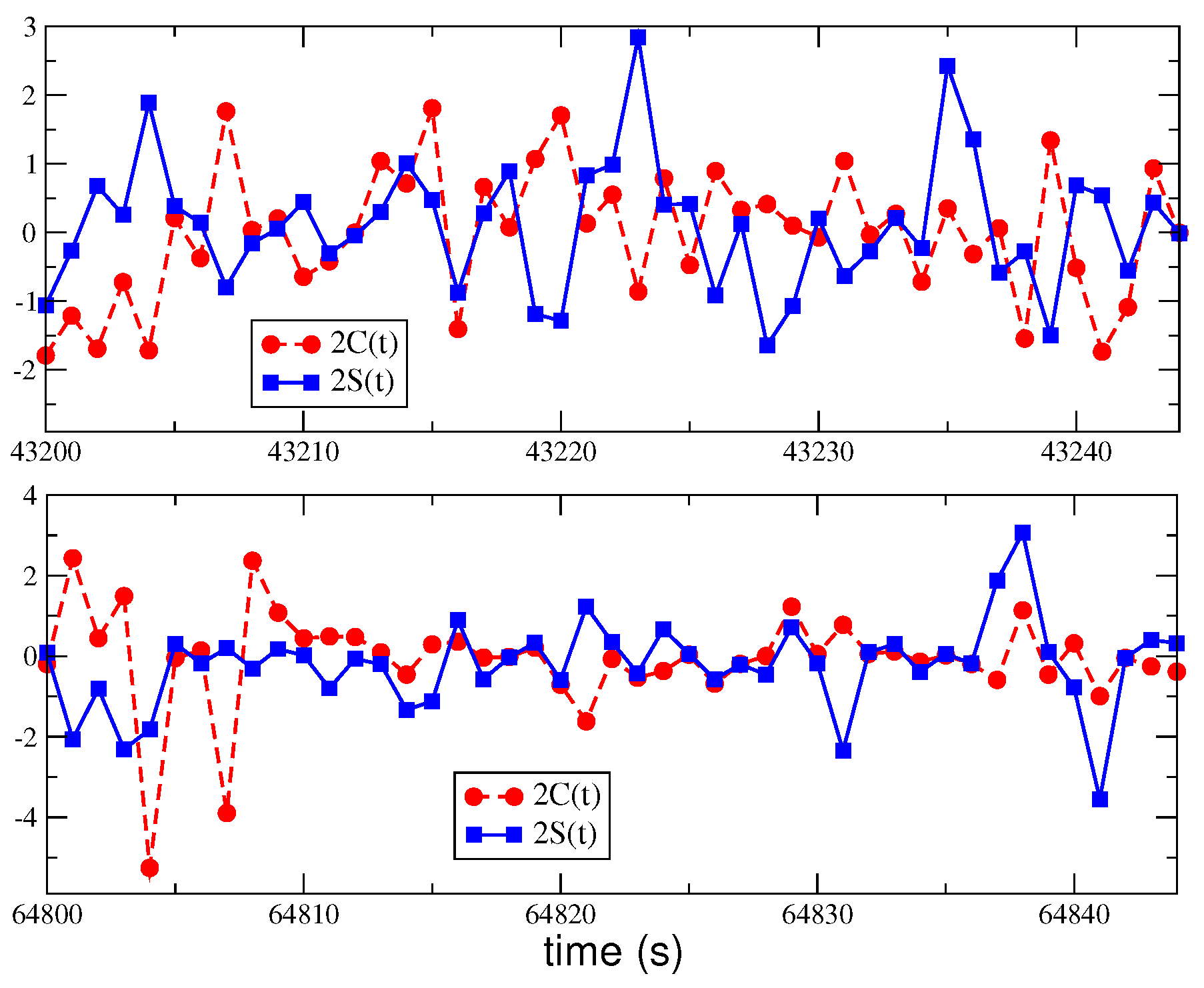
Since our signal can be approximated as a universal form of white noise and sets an intrinsic limit to the precision of measurements, for a comparison with experiments, we then considered the characteristics of the signal for the integration time (typically 1 s) in which the pure white-noise branch is as small as possible, but other types of noise are not yet important. 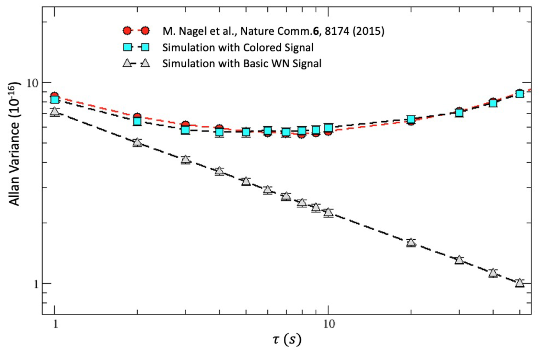In this case, when comparing with [51], our numerical simulation of the Allan variance for measurements over a whole day (${\sigma }_A{(\mathsf{\Delta }\nu ,1)}_{\mathrm{simul}}=0.26\pm 0.03$ Hz) is in complete agreement with the experimental result of ${\sigma }_A{(\mathsf{\Delta }\nu ,1)}_{\exp }\sim$ 0.24 Hz.

We also emphasized that this 0.24 Hz, when normalized to their laser frequency, gives a fractional shift of $8.5·{10}^{-16}$, which is precisely the same as that obtained in [25] at 1 s; see our Figure 13. Now, Ref. [51] is an experiment running with vacuum cavities, at room temperature, and with a reference frequency of ${\nu }_0=2.8·{10}^{14}$ Hz, while Ref. [25] is a cryogenic experiment with microwaves of 12.97 GHz, where almost all electromagnetic energy propagates in a medium (sapphire) with a refractive index of about 3. It is impossible that this extraordinary agreement can be due to accidental effects. Therefore, our conclusion is that there is a fundamental vacuum signal that shows up in vacuum and solid dielectrics and whose average magnitude is completely consistent with the velocity of 370 km/s obtained from the CMB observation with satellites in space.

We also predict periodic, daily variations in the range of $(5÷12)·{10}^{-16}$ for a typical Central European latitude. This range was obtained from our numerical simulation, but can also be expressed in a simpler way as

$${\left[{\sigma }_A(\frac{\mathsf{\Delta }\nu }{{\nu }_0},1)\right]}_t\sim 8.4·{10}^{-16}{\left(\frac{\tilde{v}\left(t\right)}{315\mathrm{km}/\mathrm{s}}\right)}^2$$

(81)

where $\tilde{v}\left(t\right)$ is defined in Equation (30). Our simulations at the end of Section 7 indicate that, for an integration time of 1 s, our basic signal is modified by about $20\%$. Therefore, these periodic variations, if they are really there, should remain visible.

Let us then return to gaseous media. Namely, what could be the physical mechanism that, starting from a fundamental ${10}^{-15}$ vacuum signal, enhances the effect up to ${10}^{-11}$ and ${10}^{-10}$ in gaseous helium and air, respectively, and finally disappears in solid dielectrics, as in the very precise cryogenic experiment in sapphire, which also gave the same ${10}^{-15}$ as in vacuum? Our answer to this question in Section 6 was based on the traditional interpretation [44,45] of the old residuals in terms of a small temperature difference $\mathsf{\Delta }{T}^{\mathrm{gas}}\left(\theta \right)$ of a millikelvin or so between the optical arms. These differences could induce convective currents of the gas molecules and a small angular dependence of the refractive index. However, we found the same universal value of $\mathsf{\Delta }{T}^{\mathrm{gas}}\left(\theta \right)=0.2÷0.3$ mK in the various experiments. Therefore, those old estimates, besides being slightly too large, were misinterpreting the effect. Since different experiments converge to the same value, the effect cannot be due to local temperature conditions, but must have a non-local origin. Our interpretation is that the interactions of the gas molecules with the background radiation are so weak that, on average, only less than 1/10 of the $\mathsf{\Delta }{T}^{\mathrm{CMB}}\left(\theta \right)$ in Equation (2) is transferred to bring the gas out of equilibrium. Nevertheless, regardless of its precise value, this thermal interpretation can help intuition by explaining the quantitative reduction of the effect in the vacuum limit where ${ϵ}_{\mathrm{gas}}\to 0$ and the qualitative difference from strongly bound solid dielectrics where this tiny thermal gradient cannot produce any observable particle motion or directional refraction in the rest frame of the medium.

In conclusion, by considering old and modern experiments, we have found several correlations between optical measurements in the laboratory and the kinematical parameters obtained from direct CMB observations with satellites in space. These correlations are summarized in the three items ((a), (b), and (c)) listed above and in the successful quantitative description of the RAV measured in [25,51] for the relevant region of integration times of about 1 s, where the white-noise branch is as small as possible, but other experiment-dependent effects are not yet important. Ours is not the only scheme to analyze the experiments, but it fulfills the traditional criterion of indicating a reference system that could play the role of the fundamental frame for relativity. We also observe that, for the same region of integration times, our scheme predicts periodic daily variations of the RAV that should be observable. Therefore, due to the importance of the issue, we would expect to receive an experimental confirmation or a disproof. If it is definitively confirmed, one more complementary test should be performed by placing vacuum (or solid dielectric) optical cavities on board of a satellite, as in the OPTIS proposal [88]. In this ideal free-fall environment, as in panel (a) of our Figure 10, the typical instantaneous frequency shift should be much smaller (by orders of magnitude) than the corresponding ${10}^{-15}$ value measured with the same interferometers on the Earth’s surface.

References

1. Penzias, A.A.; Wilson, R.W. A Measurement of Excess Antenna Temperature at 4080 Mc/s. Astrophys. J. 1965, 142, 419. [Google Scholar] [CrossRef]
2. Partridge, R.B.; Wilkinson, D.T. Isotropy and Homogeneity of the Universe from Measurements of the Cosmic Microwave Background. Phys. Rev. Lett. 1967, 18, 557. [Google Scholar] [CrossRef] [Green Version]
3. Heer, C.V. Theory for the Measurement of the Earth’s Velocity through the 3K Cosmic Radiation. Phys. Rev. 1968, 174, 1611. [Google Scholar] [CrossRef]
4. Mather, J.C. Nobel Lecture: From the Big Bang to the Nobel Prize and beyond. Rev. Mod. Phys. 2007, 79, 1331. [Google Scholar] [CrossRef] [Green Version]
5. Smoot, G.F. Nobel Lecture: Cosmic microwave background radiation anisotropies: Their discovery and utilization. Rev. Mod. Phys. 2007, 79, 1349. [Google Scholar] [CrossRef] [Green Version]
6. Yoon, M.; Huterer, D. Kinematic dipole detection with galaxy surveys: Forecasts and requirements. Astrophys. J. Lett. 2015, 813, L18. [Google Scholar] [CrossRef] [Green Version]
7. Bell, J.S. How to Teach Special Relativity, in Speakable and Unspeakable in Quantum Mechanics; Cambridge University Press: Cambridge, UK, 1987; p. 67. [Google Scholar]
8. Brown, H.R. Physical Relativity. Space-Time Structure from a Dynamical Perspective; Clarendon Press: Oxford, UK, 2005. [Google Scholar]
9. de Abreu, R.; Guerra, V. Speakable and Unspeakable in Special Relativity: Time Readings and Clock Rhythms. Electron. J. Theor. Phys. 2015, 12, 183. [Google Scholar]
10. Shanahan, D. A Case for Lorentzian Relativity. Found. Phys. 2014, 44, 349. [Google Scholar] [CrossRef]
11. Ungar, A. The relativistic composite-velocity reciprocity principle. Found. Phys. 2000, 30, 331. [Google Scholar] [CrossRef]
12. Costella, J.P.; McKellar, B.H.; Rawlinson, A.A.; Stephenson, G.J., Jr. The Thomas rotation. Am. J. Phys. 2001, 69, 837. [Google Scholar] [CrossRef] [Green Version]
13. Donnell, K.O.; Visser, M. Elementary analysis of the special relativistic combination of velocities, Wigner rotation, and Thomas precession. Eur. J. Phys. 2011, 32, 1033. [Google Scholar] [CrossRef] [Green Version]
14. Hardy, L. Quantum mechanics, local realistic theories, and Lorentz-invariant realistic theories. Phys. Rev. Lett. 1992, 68, 2981. [Google Scholar] [CrossRef]
15. Hooft, G.T. Search of the Ultimate Building Blocks; Cambridge University Press: Cambridge, UK, 1997; p. 70. [Google Scholar]
16. Consoli, M.; Stevenson, P.M. Physical mechanisms generating spontaneous symmetry breaking and a hierarchy of scales. Int. J. Mod. Phys. A 2000, 15, 133. [Google Scholar] [CrossRef] [Green Version]
17. Consoli, M.; Costanzo, E. Is the physical vacuum a preferred frame? Eur. Phys. J. C 2008, 54, 285–290. [Google Scholar] [CrossRef]
18. Consoli, M.; Costanzo, E. Precision tests with a new class of dedicated ether-drift eperiments. Eur. Phys. J. 2008, C55, 469. [Google Scholar] [CrossRef] [Green Version]
19. Consoli, M. Probing the vacuum of particle physics with precise laser interferometry. Found. Phys. 2015, 45, 22. [Google Scholar] [CrossRef]
20. Rubakov, V.A.; Tinyakov, P.G. Infrared-modified gravities and massive gravitons. Phys. Uspekhi 2008, 51, 759. [Google Scholar] [CrossRef]
21. Arraut, I. The graviton Higgs mechanism. Europhys. Lett. 2015, 111, 61001. [Google Scholar] [CrossRef] [Green Version]
22. Deser, S.; Woodard, R.P. Nonlocal Cosmology. Phys. Rev. Lett. 2007, 99, 111301. [Google Scholar] [CrossRef] [PubMed] [Green Version]
23. Soussa, M.E.; Woodard, R.P. Classical and Quantum Gravity A nonlocal metric formulation of MOND. Class. Quantum Gravity 2003, 20, 2737. [Google Scholar] [CrossRef] [Green Version]
24. Nojiri, S.; Odintsov, S.D. Modified non-local-F(R) gravity as the key for the inflation and dark energy. Phys. Lett. B 2008, 659, 821. [Google Scholar] [CrossRef] [Green Version]
25. Nagel, M.; Parker, S.R.; Kovalchuk, E.V.; Stanwix, P.L.; Hartnett, J.G.; Ivanov, E.N.; Peters, A.; Tobar, M.E. Direct terrestrial test of Lorentz symmetry in electrodynamics to 10−18. Nat. Commun. 2015, 6, 8174. [Google Scholar] [CrossRef] [Green Version]
26. Michelson, A.A.; Morley, E.W. On the Relative Motion of the Earth and the Luminiferous Ether. Am. J. Sci. 1887, 34, 333. [Google Scholar] [CrossRef]
27. Miller, D.C. The Ether-Drift Experiment and the Determination of the Absolute Motion of the Earth. Rev. Mod. Phys. 1933, 5, 203. [Google Scholar] [CrossRef]
28. Michelson, A.A.; Lorentz, H.A. Conference on the Ether-Drift Experiments. Astrophys. J. 1928, 68, 341–402. [Google Scholar] [CrossRef]
29. Illingworth, K.K. A Repetition of the Michelson-Morley Experiment Using Kennedy’s Refinement. Phys. Rev. 1927, 30, 692. [Google Scholar] [CrossRef] [Green Version]
30. Tomaschek, R. About the Michelson experiment with fixed star light. Astron. Nachr. 1923, 219, 301. (In English) [Google Scholar] [CrossRef]
31. Piccard, A.; Stahel, E. Realization of the experiment of michelson in balloon and on dry land. J. Phys. Radium 1928, IX. [Google Scholar]
32. Michelson, A.A.; Pease, F.G.; Pearson, F. Repetition of the Michelson-Morley Experiment. Nature 1929, 123, 88. [Google Scholar] [CrossRef]
33. Michelson, A.A.; Pease, F.G.; Pearson, F. Repetition of the Michelson-Morley experiment. J. Opt. Soc. Am. 1929, 18, 181. [Google Scholar] [CrossRef]
34. Pease, F.G. Ether-Drift Data. Publ. Astron. Soc. Pac. 1930, XLII, 197. [Google Scholar] [CrossRef]
35. Joos, G. Die Jenaer Wiederholung des Michelsonversuchs. Ann. Phys. 1930, 7, 385. [Google Scholar] [CrossRef]
36. Consoli, M.; Costanzo, E. From classical to modern ether-drift experiments: The narrow window for a preferred frame. Phys. Lett. A 2004, 333, 355. [Google Scholar] [CrossRef] [Green Version]
37. Consoli, M.; Matheson, C.; Pluchino, A. The classical ether-drift experiments: A modern re-interpretation. Eur. Phys. J. Plus 2013, 128, 71. [Google Scholar] [CrossRef] [Green Version]
38. Consoli, M.; Pluchino, A.; Rapisarda, A. Cosmic background radiation and ether-drift experiments. Europhys. Lett. 2016, 113, 19001. [Google Scholar] [CrossRef] [Green Version]
39. Consoli, M.; Pluchino, A. Cosmic Microwave Background and the issue of a fundamental preferred frame. Eur. Phys. J. Plus 2018, 133, 295. [Google Scholar] [CrossRef] [Green Version]
40. Consoli, M.; Pluchino, A. Michelson-Morley Experiments: An Enigma for Physics and the History of Science; World Scientific: Singapore, 2019; ISBN 978-981-3278-18-9. [Google Scholar]
41. Consoli, M.; Pluchino, A.; Rapisarda, A. Basic randomness of nature and ether-drift experiments. Chaos Solitons Fractals 2011, 44, 1089. [Google Scholar] [CrossRef] [Green Version]
42. Consoli, M.; Pluchino, A.; Rapisarda, A.; Tudisco, S. The vacuum as a form of turbulent fluid: Motivations, experiments, implications. Physica 2014, A394, 61. [Google Scholar] [CrossRef] [Green Version]
43. Shamir, J.; Fox, R. A New Experimental Test of Special Relativity. Il Nuovo Cim. B 1969, 62B, 258. [Google Scholar] [CrossRef]
44. Joos, G. Note on the Repetition of the Michelson-Morley Experiment. Phys. Rev. 1934, 45, 114. [Google Scholar] [CrossRef]
45. Shankland, R.S.; McCuskey, S.W.; Leone, F.C.; Kuerti, G. New Analysis of the Interferometer Observations of Dayton C. Miller. Rev. Mod. Phys. 1955, 27, 167. [Google Scholar] [CrossRef]
46. Müller, H.; Herrmann, S.; Braxmaier, C.; Schiller, S.; Peters, A. Modern Michelson-Morley Experiment using Cryogenic Optical Resonators. Phys. Rev. Lett. 2003, 91, 020401. [Google Scholar] [CrossRef] [PubMed] [Green Version]
47. Eisele, C.; Okhapkin, M.; Nevsky, A.Y.; Schiller, S. A crossed optical cavities apparatus for a precision test of the isotropy of light propagation. Opt. Commun. 2008, 281, 1189. [Google Scholar] [CrossRef]
48. Herrmann, S.; Senger, A.; Möhle, K.; Nagel, M.; Kovalchuk, E.V.; Peters, A. Rotating optical cavity experiment testing Lorentz invariance at the 10−17 level. Phys. Rev. D 2009, 80, 10511. [Google Scholar] [CrossRef] [Green Version]
49. Eisele, C.; Newsky, A.; Schiller, S. Laboratory Test of the Isotropy of Light Propagation at the 10−17 Level. Phys. Rev. Lett. 2009, 103, 090401. [Google Scholar] [CrossRef] [PubMed]
50. Nagel, M.; Möhle, K.; Döringshoff, K.; Schikora, S.; Kovalchuk, E.V.; Peters, A. Ultra-Stable Cryogenic Optical Resonators for Tests of Fundamental Physics. arXiv 2013, arXiv:1308.5582. [Google Scholar]
51. Chen, Q.; Magoulakis, E.; Schiller, S. High-sensitivity crossed-resonator laser apparatus for improved tests of Lorentz invariance and of space-time fluctuations. Phys. Rev. D 2016, 93, 022003. [Google Scholar] [CrossRef]
52. Consoli, M.; Pappalardo, L. Emergent gravity and ether-drift experiments. Gen. Relativ. Gravit. 2010, 42, 2585. [Google Scholar] [CrossRef] [Green Version]
53. Pound, R.V. Electronic Frequency Stabilization of Microwave Oscillators. Rev. Sci. Instrum. 1946, 17, 490. [Google Scholar] [CrossRef]
54. Drever, R.W.P.; Hall, J.L.; Kowalski, F.V.; Hough, J.; Ford, G.M.; Munley, A.J.; Ward, H. Laser phase and frequency stabilization using an optical resonator. Appl. Phys. B 1983, 31, 97. [Google Scholar] [CrossRef]
55. Black, E.D. An introduction to Pound–Drever–Hall laser frequency stabilization. Am. J. Phys. 2001, 69, 79. [Google Scholar] [CrossRef] [Green Version]
56. Guerra, V.; de Abreu, R. The conceptualization of time and the constancy of the speed of light. Eur. J. Phys. 2005, 26, S117. [Google Scholar] [CrossRef] [Green Version]
57. Maxwell, J.C. Ether, Encyclopaedia Britannica, 9th ed.; Charles Scribner’s Sons: New York, NY, USA, 1878. [Google Scholar]
58. Leonhardt, U.; Piwnicki, P. Optics of nonuniformly moving media. Phys. Rev. 1999, A60, 4301. [Google Scholar] [CrossRef] [Green Version]
59. Jauch, J.M.; Watson, K.M. Phenomenological Quantum-Electrodynamics. Phys. Rev. 1948, 74, 950. [Google Scholar] [CrossRef]
60. Kennedy, R.J. Simplified theory of the Michelson–Morley experiment. Phys. Rev. 1935, 47, 965. [Google Scholar] [CrossRef]
61. Feynman, R.P.; Leighton, R.B.; Sands, M. The Feynman Lectures on Physics; Addison Wesley Publ. Co.: Boston, MA, USA, 1963. [Google Scholar]
62. Onsager, L. Statistical hydrodynamics. Il Nuovo Cim. B 1949, 6, 279. [Google Scholar] [CrossRef]
63. Eyink, G.L.; Sreenivasan, K.R. Onsager and the theory of hydrodynamic turbulence. Rev. Mod. Phys. 2006, 78, 87. [Google Scholar] [CrossRef] [Green Version]
64. Nassau, J.J.; Morse, P.M. A Study of Solar Motion by Harmonic Analysis. Astrophys. J. 1927, 65, 73. [Google Scholar] [CrossRef]
65. Landau, L.D.; Lifshitz, E.M. Fluid Mechanics; Pergamon Press: Oxford, UK, 1959; Chapter III. [Google Scholar]
66. Fung, J.C.H.; Hunt, J.C.R.; Malik, N.A.; Perkins, R.J. Kinematic simulation of homogeneous turbulence by unsteady random Fourier modes. J. Fluid Mech. 1992, 236, 281. [Google Scholar] [CrossRef]
67. Miller, D.C. Comments on Dr. Georg Joos’s Criticism of the Ether-Drift Experiment. Phys. Rev. 1934, 45, 114. [Google Scholar] [CrossRef]
68. Swenson, L.S., Jr. The Ethereal Aether, A History of the Michelson-Morley-Miller Aether-Drift Experiments, 1880–1930; University of Texas Press: Austin, TX, USA, 1972. [Google Scholar]
69. Swenson, L.S., Jr. The Michelson-Morley-Miller Experiments before and after 1905. J. Hist. Astron. 1970, 1, 56. [Google Scholar] [CrossRef]
70. Stone, J.A.; Stejskal, A. Using helium as a standard of refractive index: Correcting errors in a gas refractometer. Metrologia 2004, 41, 189. [Google Scholar] [CrossRef]
71. Jaseja, T.S.; Javan, A.; Murray, J.; Townes, C.H. Test of Special Relativity or of the Isotropy of Space by Use of Infrared Masers. Phys. Rev. 1964, 133, A1221. [Google Scholar] [CrossRef]
72. Jennings, D.A.; Drullinger, R.E.; Evenson, K.; Pollock, C.R.; Wells, J.S. The Continuity of the Meter: The Redefinition of the Meter and the Speed of Visible Light. J. Res. Natl. Bur. Stand. 1987, 92, 11. [Google Scholar] [CrossRef]
73. Brillet, A.; Hall, J.L. Improved Laser Test of the Isotropy of Space. Phys. Rev. Lett. 1979, 42, 549. [Google Scholar] [CrossRef]
74. Numata, K.; Kemery, A.; Camp, J. Thermal-Noise Limit in the Frequency Stabilization of Lasers with Rigid Cavities. Phys. Rev. Lett. 2004, 93, 250602. [Google Scholar] [CrossRef]
75. Barcelo, C.; Liberati, S.; Visser, M. Analog gravity from field theory normal modes? Class. Quantum Gravity 2001, 18, 3595. [Google Scholar] [CrossRef] [Green Version]
76. Visser, M.; Barcelo, C.; Liberati, S. Analogue models of and for gravity. Gen. Relativ. Gravit. 2002, 34, 1719. [Google Scholar] [CrossRef]
77. Volovik, G.E. Superfluid analogies of cosmological phenomena. Phys. Rep. 2001, 351, 195. [Google Scholar] [CrossRef] [Green Version]
78. Schützhold, R. Summary of session E1 of GRG18: Analogue gravity. Class. Quantum Gravity 2008, 25, 114027. [Google Scholar] [CrossRef]
79. Consoli, M. Ultraweak excitations of the quantum vacuum as physical models of gravity. Class. Quantum Gravity 2009, 26, 225008. [Google Scholar] [CrossRef]
80. Jannes, G.; Volovik, G.E. The cosmological constant: A lesson from the effective gravity of topological Weyl media. JETP Lett. 2012, 96, 215. [Google Scholar] [CrossRef] [Green Version]
81. Finazzi, S.; Liberati, S.; Sindoni, L. Cosmological Constant: A Lesson from Bose-Einstein Condensates. Phys. Rev. Lett. 2012, 108, 071101. [Google Scholar] [CrossRef] [Green Version]
82. Yilmaz, H. New Approach to General Relativity. Phys. Rev. 1958, 111, 1417. [Google Scholar] [CrossRef]
83. Tupper, B.O.J. The Tests of General Relativity and Scalar Fields. Il Nuovo Cim. B 1974, 19B, 135–148. [Google Scholar]
84. Feynman, R.P. Superstrings: A Theory of Everything? Davies, P.C.W., Brown, J., Eds.; Cambridge University Press: Cambridge, UK, 1997; p. 201. [Google Scholar]
85. Cook, R.J. Physical time and physical space in general relativity. Am. J. Phys. 2004, 72, 214. [Google Scholar] [CrossRef]
86. Broekaert, J. A spatially-VSL gravity model with 1-PN limit of GRT. Found. Phys. 2008, 38, 409. [Google Scholar] [CrossRef] [Green Version]
87. Cella, G.; Consoli, M.; Pluchino, A. in preparation.
88. Lämmerzahl, C.; Dittus, H.; Peters, A.; Schiller, S. OPTIS: A satellite-based test of special and general relativity. Class. Quantum Gravity 2001, 18, 2499. [Google Scholar] [CrossRef]
Figure 1. A schematic illustration of the Michelson interferometer.
Universe 07 00311 g001
Figure 2. The scheme of a modern ether-drift experiment. The light frequencies are first stabilized by coupling the lasers to Fabry–Perot optical resonators. The frequencies ν 1 and ν 2 of the signals from the resonators are then compared in the beat note detector, which provides the frequency shift Δ ν = ν 1 ν 2 .
Universe 07 00311 g002
Figure 3. The observable velocity measured in various experiments reported by Miller [27].
Universe 07 00311 g003
Figure 4. The fringe shifts reported by Joos [35]. The scale corresponds to 1/1000 of a wavelength.
Universe 07 00311 g004
Figure 5. Some second-harmonic fits to Joos’ data. The figure is taken from [40].
Universe 07 00311 g005
Figure 6. Joos’ second-harmonic amplitudes in units of 10 3 . The vertical band between the two lines corresponds to the range ( 1.4 ± 0.8 ) · 10 3 . The figure is taken from [37].
Universe 07 00311 g006
Figure 7. Joos’ second-harmonic amplitudes (in units of 10 3 (black dots)) are compared with a single simulation (red diamonds) at the same sidereal times as those in Joos’ observations. Two fifth-order polynomial fits to the two sets of values are also shown. The figure is taken from [37].
Universe 07 00311 g007
Figure 8. Joos’ second-harmonic amplitudes (in units of 10 3 (black dots)) are now compared with a simulation where one averages ten measurements that were performed on 10 consecutive days at the same sidereal times as those of Joos’ observations (red diamonds). The changes in the averages observed by varying the parameters of the simulation were summarized into a central value and a symmetric error. The figure is taken from [37].
Universe 07 00311 g008
Figure 9. The experimental frequency shift reported in Figure 9a of [47] (courtesy of Optics Communications). The black dots give the instantaneous signal, the red dots give the average of the signal over 1640 sequences. For a laser frequency ν 0 = 2.82 · 10 14 Hz, Δ ν = ± 1 Hz corresponds to a fractional value Δ ν / ν 0 of about ± 3.5 · 10 15 .
Universe 07 00311 g009
Figure 10. An intuitive visualization of two physically distinct situations. In case (b), a heavy mass M is carried on board of a freely falling system. Unlike in the ideal case (a), the mass M could introduce a vacuum refractivity so that c γ c .
Universe 07 00311 g010
Figure 11. For ϵ v as in Equation (67) and z = 2 , we report in units of 10 15 two typical sets of 45 s for the two functions 2 C ( t ) and 2 S ( t ) of Equation (69). The two sets belong to the same random sequence and refer to two sidereal times that differ by 6 h. The boundaries of the stochastic velocity components in Equations (36) and (37) are controlled by ( V , α , γ ) CMB through Equations (30) and (40). For a laser frequency of 2.8 · 10 14 Hz [51], the range ± 3.5 · 10 15 corresponds to a typical frequency shift Δ ν in the range of ± 1 Hz, as in our Figure 9.
Universe 07 00311 g011
Figure 12. We report two typical sets of 2000 s for our basic white-noise (WN) signal and its colored version, which was obtained with a Fourier transform of the spectral amplitude from [25].
Universe 07 00311 g012
Figure 13. We report the Allan variance for the fractional frequency shift obtained from simulations of sequences of 2000 s for our basic white-noise (WN) signal and for its colored version, which was obtained with a Fourier transform of the spectral amplitude from [25]. The direct experimental results of [25] for the non-rotating setup are also shown.
Universe 07 00311 g013