1. Introduction
Quantitative models of magnetic fields in the Earth’s inner magnetosphere are crucial for various scientific purposes. These include the magnetic field line mapping, the evaluation of energetic particle motions and radiation belt modeling in general, as well as electromagnetic wave generation and their tracing between the observation points and source regions. The magnetic fields themselves are formed by two principally different contributions. First, it is the Earth’s internal magnetic field. Although not constant, the time scales of corresponding variations are comparatively low and this magnetic field is accurately described by a standardized International Geomagnetic Reference Field (IGRF) model [
1]. Evaluating the second contribution, originating from various currents flowing in the space plasma, is more tricky. The main reasons are its large temporal variability and complicated current systems contributing to the magnetic field. Both the location and magnitude of the individual currents need to be predicted by the respective models [
2]. These are typically parameterized by geomagnetic activity indices and solar wind parameters [
3].
An analysis of the Earth’s magnetic field deformation by impinging solar wind reveals a peculiar three-dimensional picture with a cusp region at large latitudes [
4]. The first quantitative empirical models of magnetospheric magnetic fields based on the fitting of spacecraft magnetic field measurements were developed [
5], demonstrating the dependence of the configuration on the geomagnetic activity parameterized by the Kp index [
6]. A similar approach was used by N. A. Tsyganenko to construct the, still widely used, magnetospheric magnetic model parameterized exclusively by the Kp index [
7,
8]. Newer versions of the model add an explicit magnetopause and parametrization including solar wind properties [
9,
10]. It turns out that not only the parameters at a time of interest, but also their short-term history, are important for the proper characterization of the magnetospheric magnetic fields [
9,
10]. Sophisticated coupling functions [
11,
12] are used in the newest models [
13,
14]. Ultimately, specific dynamic storm-time events with extreme magnetic field distortions [
15] might be modeled separately [
16,
17]. In a similar manner, some models aim to cover only a limited region of the magnetosphere [
18], typically close to the geosynchronous orbit [
19]. It is also feasible to reconstruct the magnetospheric configuration using global magnetohydrodynamic models, albeit only for limited time intervals [
20].
As might be expected, newer models typically perform better, in particular during geomagnetically active periods [
21]. It would seem that, already, the simple Kp-only parameterized models reasonably predict magnetic field variations, at least close to the geosynchronous orbit [
22,
23]. Magnetic field residuals between measured and model magnetic fields at these locations may eventually be lower than 3 nT for newer models [
24]. However, the model accuracy is significantly location dependent. The first few years of Cluster magnetic field data were used to show that the absolute residuals between the data and the model can reach about 20 nT near perigee. A systematic comparison of Tsyganenko magnetic field models and the first eight years of Cluster spacecraft magnetic field measurements revealed that the ring current strength is, at times, wrongly characterized by the models [
25]. The model accuracy may be further improved by employing in situ data, as demonstrated by a comparison of the performance of five different models over a time span of 21 days [
26].
In the present paper, we aim to use a large set of magnetic field measurements performed by the Cluster spacecraft between 2001 and 2018 to evaluate the accuracy of selected Tsyganenko external magnetic field models. As compared to former studies, a significantly larger dataset and four different external magnetic field models (one of them with two parametrization options) are used for the analysis. Furthermore, the accuracy of the determination of the min-B equator is investigated. The used dataset and the individual magnetic field models used are briefly introduced in
Section 2. The results obtained are presented in
Section 3 and they are discussed in
Section 4. Finally,
Section 5 contains a brief summary.
2. Data Set
Magnetic field measurements performed by the Cluster spacecraft [
27] were used in the present study. The Cluster mission consists of four identical spacecraft moving in a close constellation on similar orbits. The orbits somewhat evolved during the duration of the mission, but a typical perigee distance is about
and a typical apogee distance is nearly
. However, due to the slight orbital changes over the course of the mission, the entire region of the Earth’s inner magnetosphere is effectively covered. The mission started in 2001, and it is still active. We used the data measured in 2001–2018. The used three-component vector magnetic field data were obtained by a flux–gate magnetometer (FGM) instrument onboard [
28]. The time resolution of the measurements depends on the mode of the instrument. However, for the purpose of the presented study, the spin time resolution (about 4 s) available essentially continuously is sufficient. In fact, it is quite certainly better than needed. However, since the calculation is manageable even with this fine time resolution, we opt not to artificially decrease it by additional averaging.
Magnetospheric magnetic field models Tsyganenko 89 (T89, [
8]), Tsyganenko 96 (T96, [
29,
30]), Tsyganenko 01 (T01, [
9,
10]), Tsyganenko and Andreeva 15B, and Tsyganenko and Andreeva 15N (TA15B and TA15N, [
13,
31]) are implemented as a part of the Geopack library [
32,
33]. We note that the TA15B and TA15N models have the same mathematical structure and they essentially differ only in a coupling function used. The TA15B model is parameterized by a coupling index
[
12], while the TA15N model is parameterized by a coupling index
[
11]. In order to run the considered models properly, geomagnetic activity indices (Kp for T89, Dst for T96 and T01) as well as solar wind parameters for T96, T01, TA15B, and TA15N (dynamic pressure, IMF
, and IMF
) and eventually their history for T01 (
and
indices) and coupling indices for TA15B and TA15N (
and
indices) are needed. For this purpose, we used OMNI solar wind parameters, which provided a convenient propagation of the parameters from a solar wind monitor to the bow shock nose. Given the nature of the intended calculations, OMNI data with a 5-minute time resolution seem to be the best suited for our analysis. Input parameters needed to run the TA15B and TA15N models were provided by the authors of the models [
34].
Magnetic field data from a given Cluster spacecraft were considered in the analysis only if they were measured at the time when the spacecraft was safely inside the model magnetopause, thus omitting the data possibly measured in the magnetosheath. For this purpose, an empirical magnetopause model [
35] was used and all measurements outside the model magnetopause or at radial distances within 1
from the model magnetopause were excluded from the analysis. Additionally, only the Cluster magnetic field data, for which all necessary solar wind parameters were available to correctly run all the external magnetic field models (T89, T96, T01, TA15B, and TA15N), were included in the analysis. Although dedicated interpolation methods in principle allow us to overcome small data gaps with reasonable accuracy [
36], we opted not to do so as we focused on the model performance itself and needed to minimize the bias introduced by possibly imprecise input parameters. Moreover, in order to prevent the model usage under too extreme situations, which are typically beyond the recommended parameter ranges for individual models, such data intervals were excluded from the analysis. Specifically, only the data measured at the times of solar wind dynamic pressure between 0.5 and 10 nPa, Dst between −100 and 20 nT, and IMF
and
between
and 10 nT were used. Additionally, the coupling indices
and
used, respectively, by the TA15B and TA15N models, were required to be between 0 and 2. Altogether, this left us with ≈200 millions of vector magnetic field measurements with the 4 s time sampling obtained by the four Cluster spacecraft during 2001–2018. We note that, for this purpose, individual Cluster spacecraft measurements were treated independently, that is, the fact that the Cluster spacecraft typically fly in a rather close constellation was not exploited in this part of the analysis.
The model vector magnetic fields were evaluated for each of the measured data points using all the considered external magnetic field models. The model magnetic fields were calculated as a vector sum of the Earth’s internal magnetic field predicted by the IGRF magnetic field model [
1] and respective external magnetic field contributions. Five model vector magnetic fields,
,
,
,
, and
were thus attributed to each measured magnetic field vector
.
The four-point Cluster magnetic field measurements allowed us to use a linear interpolation method to determine the gradient and magnetic field in the center of the Cluster constellation [
37]. The location of the min-B equator, where the magnetic field along a given field line reaches a minimum, could be then determined. It is the location where the projection of the gradient of the magnetic field strength onto the direction of the magnetic field is equal to zero [
38]. This type of analysis thus requires the entire Cluster spacecraft constellation to pass through the min-B equator, with continuous magnetic field measurements being available. Altogether, 332 such equatorial crossings occurred during the analyzed period with the aforementioned conditions on the OMNI data availability and values and distance from the magnetopause applied. Moreover, considering that the method of the linear interpolation became inherently inaccurate for larger spacecraft separations, we limited the analysis to only the crossings for which the distance of all spacecraft from the center of the constellation was lower than 0.25
. This left us with 101 Cluster constellation crossings of the magnetic equator.
3. Results
All the analyses were performed in geocentric solar magnetic (GSM) coordinates. We further assume that the situation was symmetric with respect to the GSM plane, that is, that there were no systematic differences between the results obtained for positive and negative Z values. This allows the results to be plotted as a function of the absolute value of the Z coordinate. Moreover, a dawn–dusk symmetry is assumed. Although these assumptions are clearly rather bold, they allow us to reasonably limit the number of resulting plots, while keeping the main characteristic intact. The local time dependence is then expressed by considering only three local time bins. These local time bins are defined based on the azimuthal angle in the GSM coordinates and the following bins are used: day (9–15 h), dawn/dusk (3–9 and 15–21 h), and night (21–24 and 0–3 h).
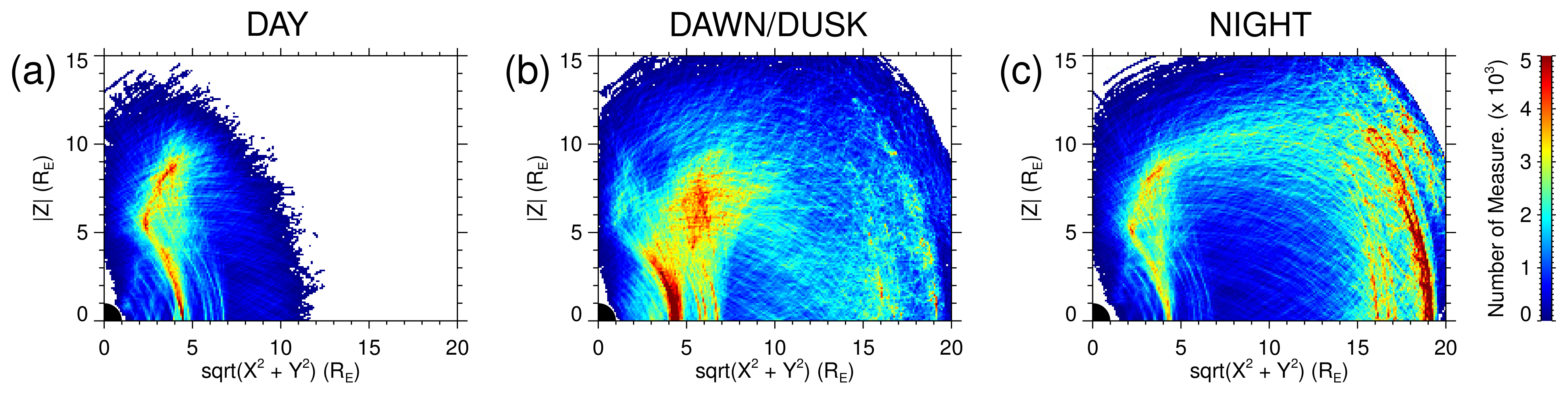
The number of measurements in individual
large bins in
(abscissa) and
(ordinate) analyzed in the three local time intervals is color coded in
Figure 1 according to the color scale on the right-hand side. It can be seen that the entire region of the inner magnetosphere is well covered, with more measurements being obtained close to the equatorial region at radial distances of about 4
(and 19
for the nighttime). The lack of dayside measurements at larger radial distances is due to the omitting of data measured outside or close to the model magnetopause location.
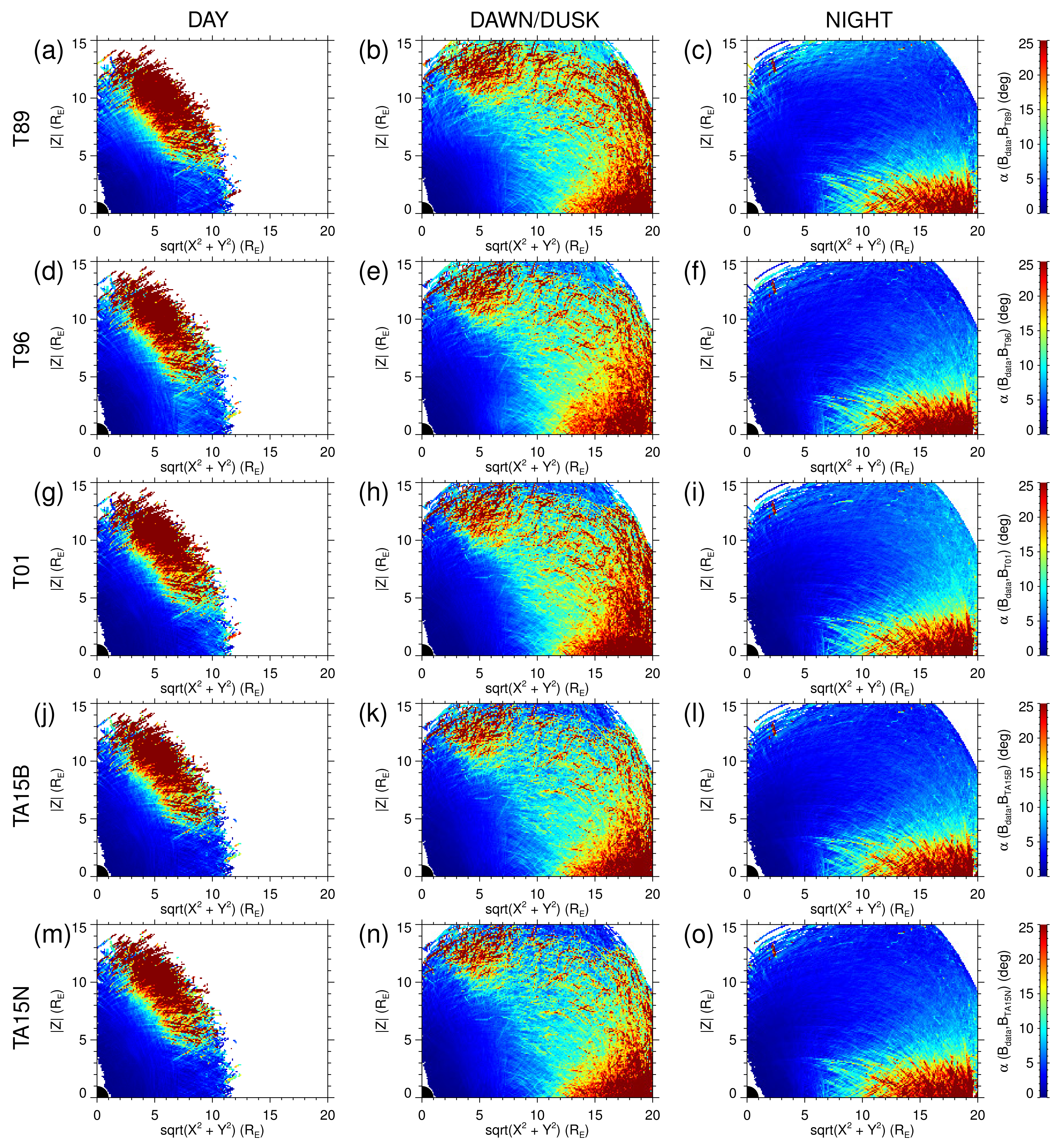
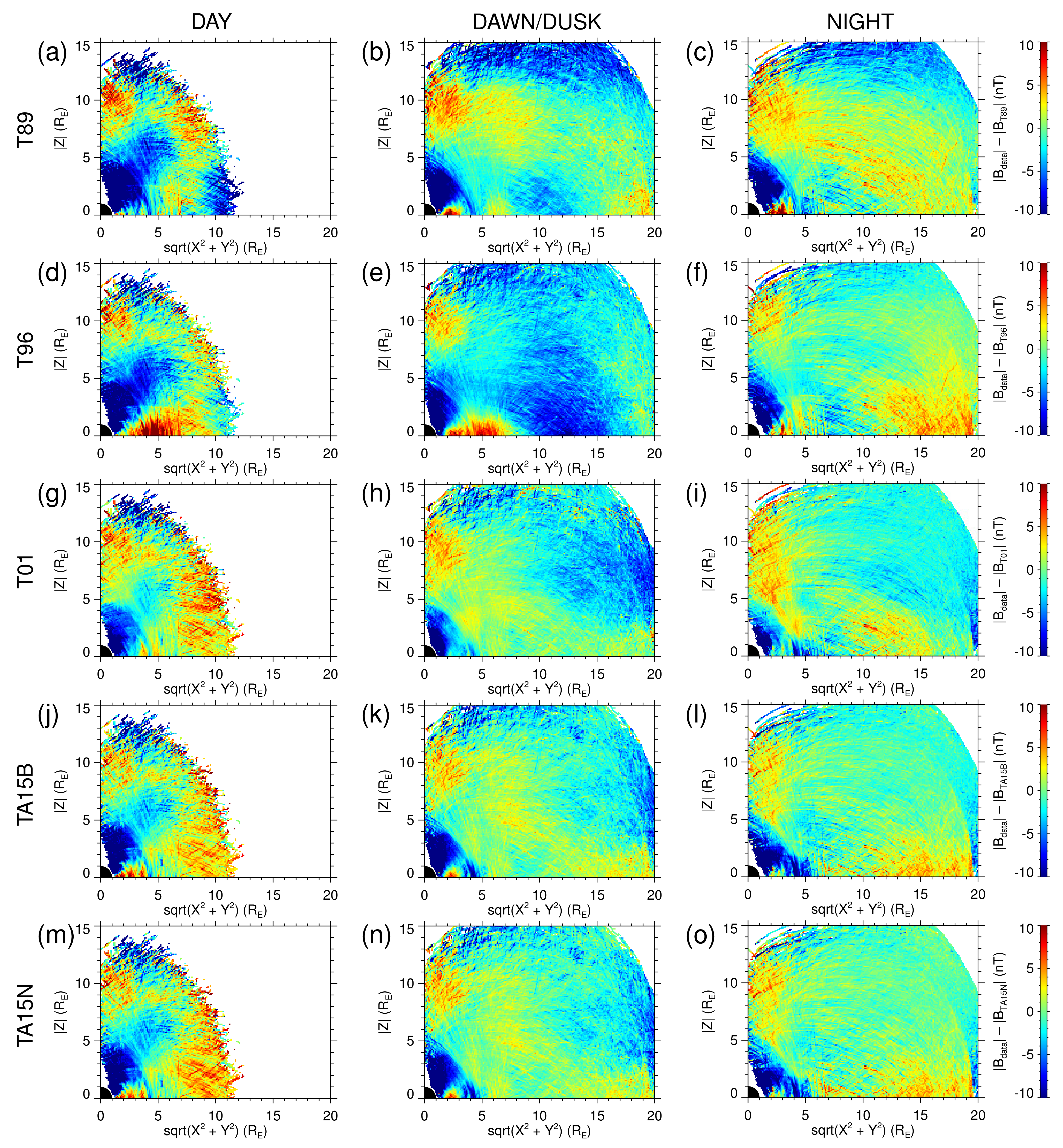
Both the measured and model magnetic fields are vector quantities, the comparison of which is a bit less straightforward than a comparison of scalar values. Three possible approaches to how to quantify the accuracy of the model magnetic fields are used. First, the magnitudes of the measured and model magnetic field vectors are compared in
Figure 2. Second, the angular differences between the measured and model magnetic field vectors are evaluated in
Figure 3. Third, the magnitudes of vector differences between the measured and model magnetic field vectors are studied in
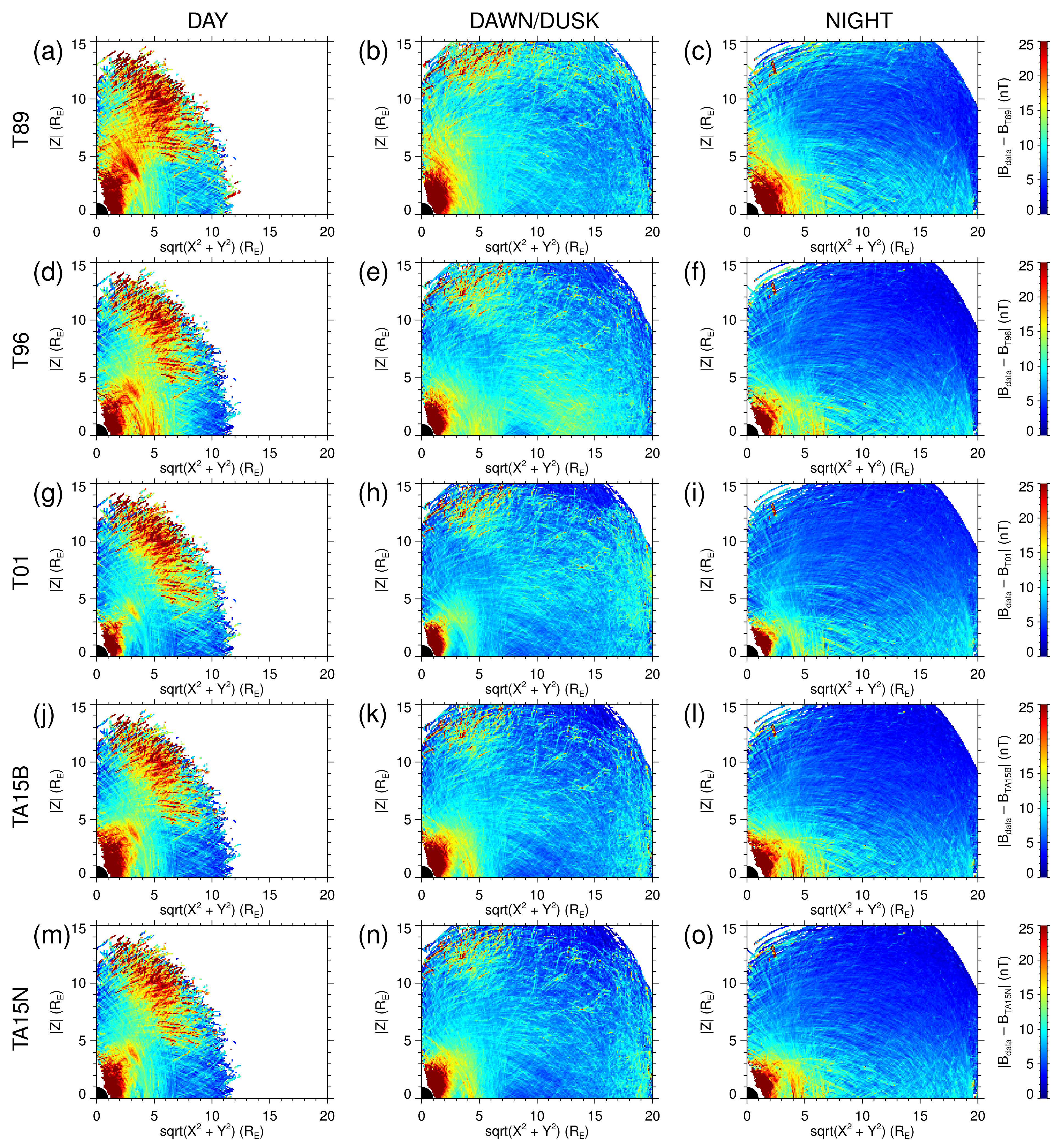
Figure 4. All the figures use the same format, containing fifteen panels organized in five rows and three columns. Each column corresponds to a different local time, that is, respectively, day, dawn/dusk and night. Each row corresponds to a different external magnetic field model used, that is, respectively, T89, T96, T01, TA15B and TA15N. The average differences between the measured and model magnetic fields are color coded in individual
large spatial bins using the color scale on the right-hand side.
Figure 2 compares the measured and model magnetic field magnitudes by evaluating the average differences between them. The red color thus corresponds to the measured magnetic field magnitude being larger than the model magnetic field magnitude, while the blue color corresponds to the measured magnetic field magnitude being lower than the model magnetic field magnitude. It can be seen that the differences are typically within about 10 nT, being somewhat lower and more uniform for the T01, T15B and T15N models than for the T89 and T96 models. The performances of the T01, T15B and T15N models seem to be roughly the same. However, some systematic deviations can be identified. At low radial distances, the model magnetic field magnitudes are higher than the measured magnetic field magnitudes for all models and all local times. The corresponding region is apparently more limited for the T01 model and for the nightside situation. At larger radial distances and latitudes, the model magnetic fields are systematically lower than the measured magnetic fields. Again, the difference is apparently the largest for the T89 model. The third region of significant systematic differences of measured and model magnetic field magnitudes is identified in the equatorial region at radial distances of about 5
. It occurs exclusively for the T96 magnetic field model, which considerably underestimates the magnetic field magnitudes in this region. This indicates that the ring current is at times wrongly characterized by the T96 model, in agreement with former results [
25].
Figure 3 uses the same format as
Figure 2 to depict average angular differences between the measured and model magnetic field directions. These dependences are quite comparable for all the external magnetic field models. At lower radial distances, where the total magnetic field is strongly dominated by the Earth’s internal magnetic field, the angular deviations are very low. They gradually increase with increasing radial distances, and they eventually exhibit two locations where the magnetic vector orientations are only poorly described by the models. First, it is the region on the dayside at large latitudes, corresponding to the cusp region. Second, it is the equatorial region at larger radial distances on the nightside, corresponding to the current sheet. It is understandable that the exact magnetic field configuration in these two regions is very sensitive to the details of external forcing, and an accurate empirical characterization of the magnetic field orientation therein is thus quite impossible. Given the rather large local time intervals used, the influences of these two particular problematic regions eventually also extend to the dawn/dusk side.
Average magnitudes of vector differences between the measured and model magnetic fields are investigated in
Figure 4. It can be seen that the largest differences are observed at low radial distances. This is consistent with the results shown in
Figure 2. Another problematic region corresponds to the cusp region at larger radial distances and latitudes, in line with the features identified in
Figure 3. However, the uncertainty in the magnetic field directions in the current sheet manifested in
Figure 3 is significantly suppressed in the representation used in
Figure 4. The reason is that, although the magnetic field directions tend to be predicted quite inaccurately, the magnetic field magnitudes are comparatively low and so are thus the corresponding magnitudes of the magnetic vector differences. Apart from these global features,
Figure 4 shows quite clearly that the magnitudes of vector differences tend to be systematically lower for newer magnetic field models.
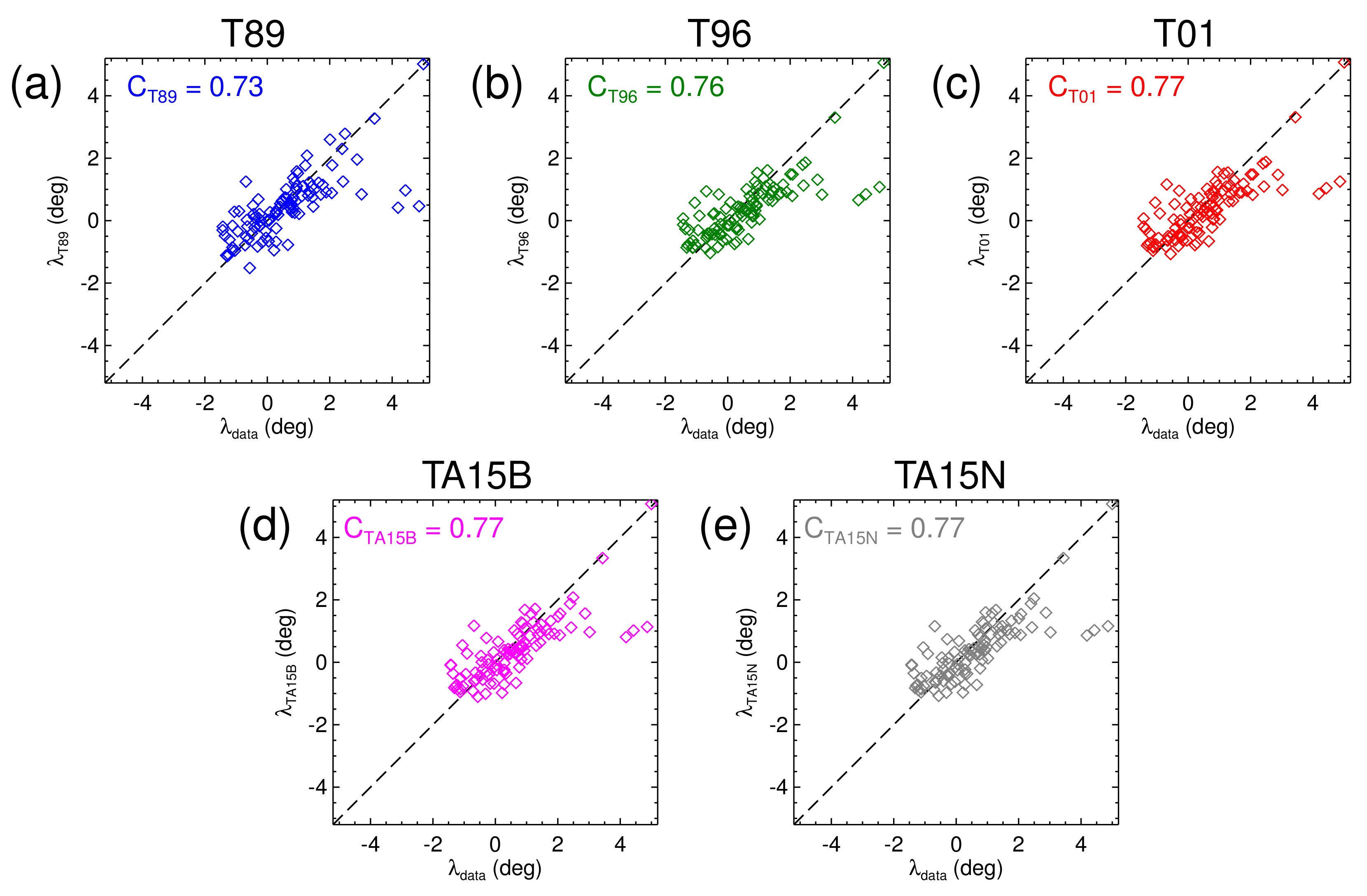
Geomagnetic latitudes of the min-B equator determined based on the four-point Cluster spacecraft measurements and from the magnetic field models are compared in
Figure 5. The results obtained for the T89, T96, T01, TA15B and TA15N magnetic field models are plotted in
Figure 5a–e, respectively. Each symbol corresponds to a single equatorial crossing of the Cluster spacecraft constellation. The dashed diagonal lines show 1:1 dependences, and the respective Pearson correlation coefficients are shown at the upper left corners of the individual panels. It can be seen that the correlations obtained for all the models are quite comparable, about 0.7–0.8. However, the newer models appear to work slightly better than their predecessors. It is worth noting that there is a small group of min-B equators at apparently quite large geomagnetic latitudes based on the four-point measurements, which is not well captured by neither of the models (although the newer models capture it arguably somewhat better). We cannot exclude the possibility that these particular min-B equator locations are badly determined from the Cluster four-point measurements for some reason.
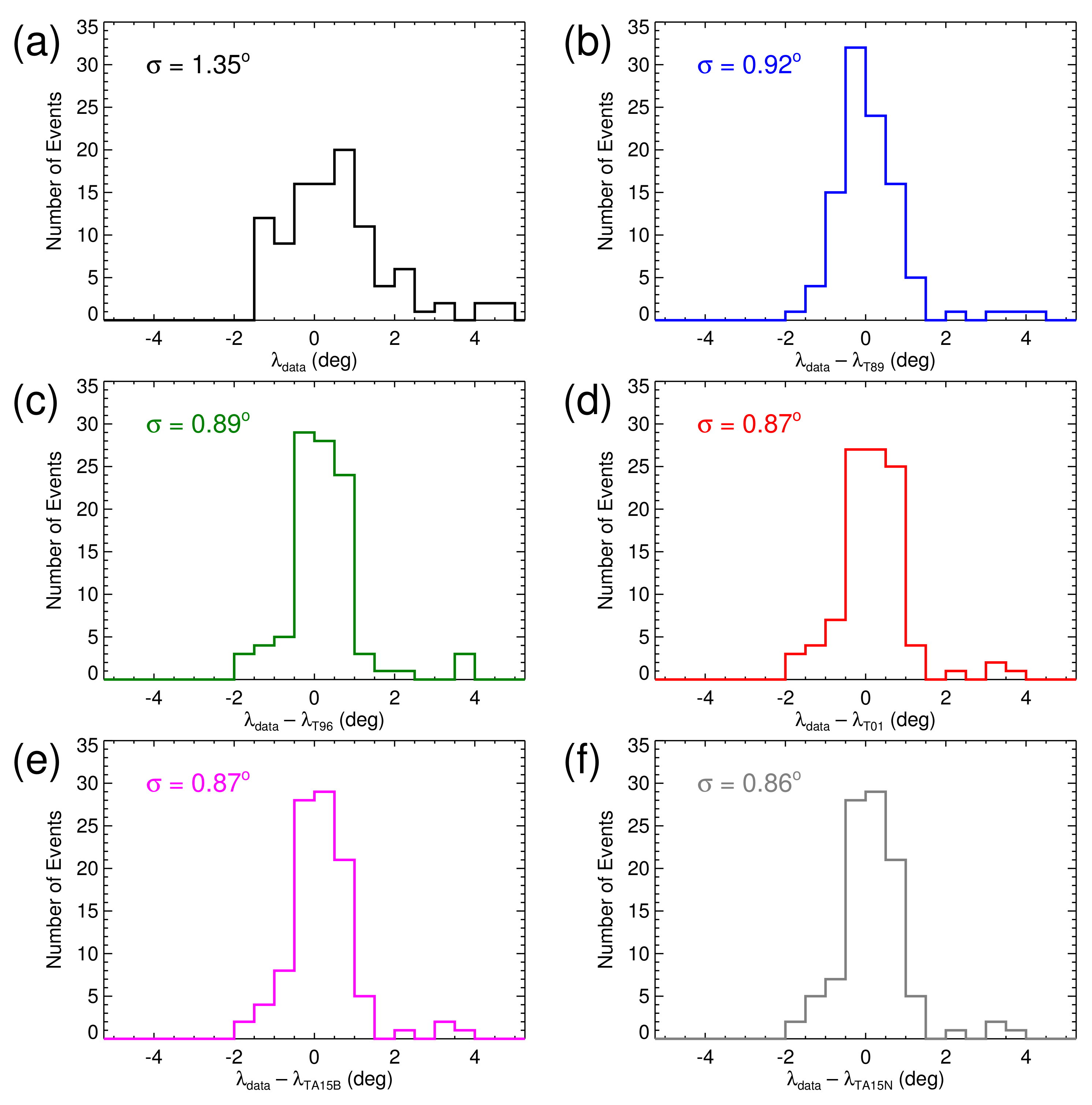
A distribution of geomagnetic latitudes of min-B equators in terms of histograms is analyzed in
Figure 6.
Figure 6a shows a histogram of geomagnetic latitudes where min-B equators occur according to four-point Cluster magnetic measurements. It can be seen that they are symmetrically distributed around the geomagnetic equator, with the respective geomagnetic latitudes being generally lower than about two degrees. There is the aforementioned exception of the small group of min-B equators at comparatively large geomagnetic latitudes.
Figure 6b–f shows histograms of geomagnetic latitude differences between the min-B equators determined based on the Cluster measurements and based on the T89, T96, T01, TA15B and TA15N magnetic field models, respectively. If both the determination of the min-B equator from the Cluster spacecraft data and the models worked perfectly, then these distributions should essentially correspond to a delta function, with a clear extra sharp peak at zero latitudinal difference. It can be seen that this is not fully the case, although the distributions eventually get somewhat narrower than the latitudinal distribution in
Figure 6a. The performances of all the magnetic field models seem to be roughly comparable, as is also confirmed by the standard deviations shown at the top left of the individual plots. Finally, we note that the min-B equator locations determined using the four-point Cluster measurements used as a benchmark are clearly not completely accurate, and as such they are responsible for at least a part of the observed latitudinal scatter.
4. Discussion
Vector magnetic field measurements performed by the four Cluster spacecraft analyzed in the present paper represent a unique dataset, allowing us to systematically evaluate the performance of some widely used inner magnetospheric magnetic field models. Although the spatial coverage is necessarily not uniform, they conveniently cover principally the entire region of the Earth’s inner magnetosphere. Additionally, the four-point measurements allow us, at least at the times of close spacecraft separations, to experimentally determine the crossing of the min-B equator. This is another metric that is important when evaluating the accuracy of magnetic models, which is especially important with regard to the wave–particle interactions taking place there [
39].
Given that both the measured and model magnetic fields are vector quantities, several possibilities of their comparison are suggested and applied. First, the differences between measured and model magnetic field magnitudes are evaluated, which is a simple metric useful for assessing basic plasma parameters, such as the cyclotron frequency. Second, the angular differences between the measured and model magnetic vectors are important for the global shape of the magnetic field configuration and the Earth’s magnetic field deformation due to the interaction with the solar wind. Third, the magnitudes of the vector differences between the measured and model magnetic field vectors are in some sense a combination of the two, reflecting both the inaccuracies in the magnitude and direction.
The analysis of the aforementioned three accuracy metrics as a function of the location and local time revealed some important and, to an extent, systematic differences. Although the newer models are generally, at least globally, more accurate, three problematic regions eventually remain. The first of them is located at lower radial distances, where the measured-model magnetic field differences tend to be quite high in absolute values. Nevertheless, considering that the magnetic field magnitude therein is high, the relative differences are comparatively small. The second problematic region is located at larger latitudes and larger radial distances, corresponding essentially to the cusp [
40]. Although it is manifested in all the three metrics used, it appears to be most pronounced in the angular differences between magnetic field directions. The same holds for the third problematic region, which is located at larger radial distances and low latitudes, corresponding to the plasma sheet. In this region, the magnetic field magnitudes are typically predicted rather well, but the determination of the magnetic field orientations tends to be inaccurate.
Evaluating the accuracy of the min-B equator determination is more complicated, as its location cannot be directly measured (the spacecraft do not move along magnetic field lines). Instead, the min-B equator latitude needs to be determined based on four-point Cluster measurements and the magnetic field gradient estimated in the center of the tetrahedron configuration. Such a method is necessarily less accurate for larger spacecraft separations, which were omitted from the analysis. A comparison of the min-B equator locations determined in this way, with the min-B equator locations determined using external magnetic field models, reveals a good overall correlation between the two. Moreover, the agreement appears to be slightly better for the newer magnetic field models, suggesting that they indeed perform somewhat better also in this regard. Nevertheless, the differences up to about one degree still remain.
5. Conclusions
Long-term vector magnetic field measurements performed by the four Cluster spacecraft during 2001–2018 allowed us to systematically compare measured and model magnetic field vectors in the Earth’s inner magnetosphere. Only the data measured at radial distances safely lower than the magnetopause stand-off distance were used in the analysis. IGRF Earth’s magnetic field model and four different external magnetic field models (T89, T96, T01, TA15), where the TA15 model was used with two parametrization options (TA15B, TA15N), were used for the comparison. Differences in measured and model magnetic field magnitudes, magnetic vector orientations and magnitudes of vector differences were evaluated as a function of the spacecraft location and local time. It was shown that, although the newer models perform generally better than the old ones, some systematic deviations remain, in particular at larger geomagnetic latitudes. Additionally, the four-point Cluster spacecraft measurements allowed us to experimentally determine the locations of the min-B equator. The respective magnetic latitudes were compared with the magnetic latitudes of min-B equator determined based on the individual external magnetic field models. It was shown that, although the newer models appear to perform slightly better, an uncertainty of about one degree in the determination of the min-B equator latitude remains.


