Abstract
We calculate the vacuum (Casimir) energy for a scalar field with self-interaction in (1 + 1) dimensions non perturbatively, i.e., in all orders of the self-interaction. We consider massive and massless fields in a finite box with Dirichlet boundary conditions and on the whole axis as well. For strong coupling, the vacuum energy is negative indicating some instability.
1. Introduction
The notion of vacuum energy results from the ground state of a quantum system, particle, or field. This is the state with no excitations. As known since early quantum mechanics, the energy of a harmonic oscillator,
has a resudial amount,
which is called zero-point energy. Since in quantum field theory the groundstate is called vacuum state, or simply vacuum, this energy is called vacuum energy. The necessary sum over the degrees of freedom of a field,
makes the vacuum energy, of course, infinite. While this was a problem in earlier times, by now powerful methods of regularization and renormalization are known, notably the zeta functional regularization and the renormalization assisted by the heat kernel expansion. The regularized vacuum energy,
with at the end, is finite and does exist, in distinction from (3). The known price to be paid is the appearance of the arbitrary parameter .
The simplest example known is a free scalar field in a box with Dirichlet boundary conditions. It has eigenfrequencies
and its vacuum energy is
In this case, the continuation to is done by the Riemann zeta function and there was no pole term (which is, of course, not the general case). For a detailed explanation of the renormalization procedure, we refer to the appropriate literature, the book [1], Section 4.3, for instance.
A characteristic feature of the vacuum energy (6) is that it vanishes for . This is not surprising for two reasons. First, for dimensional reasons, and second, from the interpretation as the vacuum energy change brought in by the boundaries. Accordingly, there is a general expectation that the vacuum energy makes sense only relative to the empty space.
It must be mentioned that this remark touches on a principal question. Let us start from zero-point energy in quantum mechanics, say of one harmonic oscillator. Its ground state energy cannot be measured from experiments that were sensitive to a change in the energy levels, say by spectroscopy, but only by a change of the intrinsic frequency of the oscillator. The first detection of zero-point energy this way is known from early quantum mechanics as a difference in vapor pressure between certain neon isotopes (see the contribution by Rechenberg in [2]). This feature slipped over to quantum field theory. What we can measure is always a change in energy, resulting in a force or pressure. The same holds also for the gravitational action. An attempt to give the vacuum energy of the empty space a physical meaning by introducing a cut-off, results in the known, too large by far, estimates for the cosmological constant (see, e.g., [3]). Recently, this topic was discussed from a modern point of view in [4].
To date, it was not possible to attribute, in a meaningful way, vacuum energy to the empty space. As mentioned, the reason can be seen in the lack of a dimensional parameter. In the present paper, we demonstrate a simple example where we have such a parameter in empty (and flat) space. We consider a real scalar field in (1 + 1) dimensions with the action
obeying, after Fourier transform in time, a non-linear Schrödinger Equation (NLS),
The coupling has the dimension length . As known, in the perturbative approach this model is super-renormalizable.
We start with a finite box with Dirichlet boundary conditions,
resulting in discrete frequencies , and we calculate the vacuum (Casimir) energy generalizing (6). Continuing, it turns out that the limit can be performed in a meaningful way delivering the vacuum energy of a field with self-interaction in flat, empty space. This way, for the first time, the vacuum energy for a quantized field in flat, empty space is calculated. The key point is the self-interaction of the field, providing the necessary dimensional quantity.
It must be mentioned that the overwhelming majority of vacuum energy and Casimir force calculations were done for free fields with the ’only’ complication of boundaries and/or background fields. Of course, for decades this was a serious problem. So, for example, it took 20 years to generalize the original calculation of Casimir [5], which was for flat, parallel plates, to a sphere [6], and nearly 30 more years until the first calculation of vacuum energy in a three-dimensional background field [7]. For interacting fields, there are so far only perturbative calculations. Starting from a scalar field in a rectangular cavity, for example [8,9], over the electron field on a spherical boundary [10], up to, recently, various improvements of the renormalization procedure [11] and a very recent perturbative calculation in [12]. We mention that also in [13] the quantum fluctuations were described by a free field.
From the point of view of quantum field theory we proceed as follows. The solutions of the field Equation (8) form a complete set and the expansion
holds with the corresponding eigenvalues . As stated in the papers [14,15], these solutions form a complete set. Further we apply the standard canonical quantization procedure turning the into operators with the usual commutation relations. As a result we arrive at the vacuum energy (4). In short, we ’merely’ substitute the usual plane waves by the functions .
In the present paper, we remind the basic formulas for the solutions of the NLS (8). These were investigated in many papers and under many aspects, including the inverse scattering method. There is rich and beautiful physics connected with these solutions, which we do not touch at all in this paper. We use the explicit solutions in terms of Jacobi elliptic functions, which were investigated in the papers [14,15,16], and also in the very recent [17]. Subsequently, we remind some basic facts from the renormalization of vacuum energy. Finally, we calculate some examples and discuss the strong coupling behavior.
Throughout the paper, we use natural units with . Further, we use the standard notations for the Jacobi elliptic functions as used, for instance, in [18] with m in place of the parameter , such that and . Since m is a standard notation in this context, we use the notation for the mass (irrespective of whether ’e’ denotes an electron or not).
2. Solutions of the NLS in Terms of Elliptic Functions
As shown in Appendix B in [19], any solution of (8) can be expressed in terms of one of the Jacobi elliptic functions. The specific choice is, then, motivated by the boundary conditions. It is meaningful to consider the cases and separately. We start with the repulsive one, i.e., with .
2.1. The Repulsive Case
We make the ansatz
We mention that is that elliptic function which generalizes . The boundary condition (9) in is satisfied by the choice of the elliptic function . The boundary condition in demands
where is the complete elliptic integral of the first kind, which is a quarter period of . A and m are still free parameters. We insert the ansatz into Equation (8) which we preliminarily rewrite in the form
Multiplying by we get with (12) the first integral,
where C is an integration constant. With Equation (22.13.1) from [18], we arrive at
Comparing equal powers of , the relations
follow. Another relation emerges from the normalization condition which one must impose,
and which with (11) takes the form
Here we apply Equation (5.134 1) from [20] to get
where is the amplitude. It obeys
where is the complete elliptic integral of second kind, and (18) turns into
Inserting from (16) and (12) delivers the equation
This is an equation for the parameter m and we denote the solutions by . Then the frequencies become also discrete and from (16) we find
The calculation of these frequencies is quite easy since the right sides of (22) and (23) are monotone functions.
The , (23), are the eigenfrequencies of the field obeying the boundary conditions (9) and enter the vacuum energy (4). Below we will need their behavior for large j. Expanding the mentioned right sides in powers of m, one comes to the perturbative (in ) expansion
The leading order gives just the well-known eigenfrequencies of a free field in a box. The behavior for large follows from (22) with the remark that the elliptic integrals grow logarithmically for . Using the corresponding asymptotic expansions,
follows for fixed j.
2.2. The Attractive Case
In distinction from the preceding subsection, we assume now (we do not substitute ). Following [15], we make the ansatz
with the elliptic function which generalizes the cosine function. To fulfill the boundary condition (9) one must take the choice
Further, the discussion goes completely in parallel to the preceding case. In place of (14) we have now
With Equation (22.13.2) from [18] we arrive at
and comparing equal powers of results in the relations
Here one can understand the choice of the ansatz (26) since negative in (16) would give an imaginary prefactor A. For the integration in the normalization condition, we use now Equation (5.134 2) from [20],
and with (27) we arrive at
Inserting for A from (30) delivers the equation
whose solutions are the ’s in the case (we do not introduce a separate notation). Finally, from (30), the eigenfrequencies follow to be
For large numbers j, the same expansion (24) as in the repulsive case holds. The behavior for large is different from the preceding case. While, again, from the right side of (33), follows, the frequencies become imaginary as soon as m exceeds . The critical value is (The right side is within a numerical precision of at least 100 digits just . I’m indebted to the first referee for this hint.)
This means that the attractive self-interaction makes the system unstable if the coupling exceeds some critical value, which is, of course, an expected feature.
3. The Vacuum Energy in a Finite Box
The vacuum energy is, in zeta functional regularization, given by Equation (4). In the case of a massive field, obeying the equation
as we consider it here, it reads
with the eigenfrequencies as given by (23) for and by (34) for . In the latter case, when is imaginary, still a stable solution exists as long as holds. Imaginary act similar to bound states in this context. Denoting the left side of (33) by t, this equation defines a function . Then the critical is solution of the equation
and the condition of stationarity reads
For we come to (35).
The renormalization procedure is, in general, well-known. We follow the mentioned chapter in [1], and formulas adopted to the (1 + 1)-dimensional case in the recent [21]. First, we need to define the zeta function associated with our spectrum . It reads
The pole parts, which we need for the heat kernel coefficients, follow from inserting the asymptotic expansion (24),
where, as already mentioned, is the Riemann zeta function. The heat kernel coefficients are expressed by the residua,
and those relevant for the renormalization read
As usual, is the volume of the empty space. The coefficient is, may be occasionally, the same as in [21] and we refer to the remark in the paragraph following Equation (81) in that paper. The coefficient is the deciding one for the renormalization. It is non-zero with the known consequences. In passing, we mention that it is zero for which explains the finite result (6).
The renormalization is performed by subtracting the contributions from the heat kernel coefficients (43) to . Using the (1 + 1)-dimensional modification of Equation (4.30) in [1], we define
As known, the heat kernel expansion provides an asymptotic expansion of the vacuum energy in inverse powers of the mass and (44) collects all non-decreasing powers. We define the renormalized vacuum energy by
such that it vanishes for . This is a kind of normalization condition based on the argument that a ’heavy’ quantum field should not have vacuum fluctuations. At once, this way the regularization ambiguity, which came in with the parameter , drops out (see below, Equation (51)).
We mention that the poles in s are the only ultraviolet divergences in the considered model. For instance, these are at most first order in the coupling in agreement with the superrenormalizability of the model.
In order to perform the continuation in (45), we use the asymptotic expansion (24) to split the regularized vacuum energy into two parts,
with a ’leading’ contribution,
and
In the last expression we could put since the sum converges. Note, is to be calculated from (23) for and from (34) for . Numerical evaluation does not pose problems.
Rearranging (45) and using (46), we arrive at
with
Inserting (44) into (47) we get
Representation (49) holds for both signs of the coupling . It can be evaluated numerically. Examples are shown in Figure 1 and Figure 2. For , together with , the free case (6) is recovered. The same holds for .
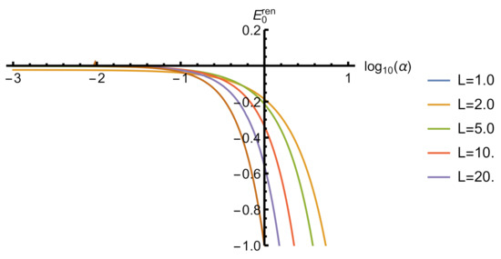
Figure 1.
The vacuum energy of a massive scalar field in a box with repulsive self-interaction. All quantities are given in units of the mass .Spectrum
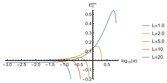
Figure 2.
The vacuum energy of a massive scalar field in a box with attractive self-interaction with . The curves terminate where the energy becomes complex. All quantities are given in units of the mass .Spectrum
For the massless case, the renormalization procedure is slightly different. As known, and as can be seen from (51), the limit is logarithmically divergent. In the massless case, the argument with the large mass expansion is not applicable and, without further considerations, the result will depend on , thus it will be not unique. In this paper, we do not discuss possible normalization conditions in the massless case and keep the -dependence of the result.
For , the vacuum energy has a pole term resulting from in (44) or, equivalently, from in (47). It reads
For the renormalization we simply subtract this pole contribution and define, in analogy to (50),
Furthermore, we split, in parallel to (46)
where is given by (47) and by (48), both with . Rearranging, we come to
with
( is Euler’s gamma). Examples are shown in Figure 3 and Figure 4.
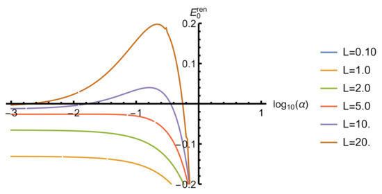
Figure 3.
The vacuum energy of a massless scalar field in a box with repulsive self-interaction and . and are given in units of .Spectrum
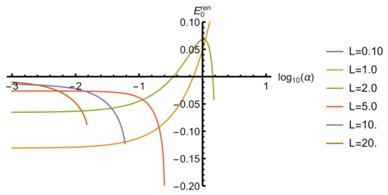
Figure 4.
The vacuum energy of a massless scalar field in a box with attractive self-interaction and . The curves terminate when the energy becomes complex. and are given in units of .Spectrum
4. The Infinite Volume Case
By taking the limit we come to the infinite volume case. In this limit, first of all, we mention that for we always have an imaginary frequency since (39) cannot be fulfilled for any finite and j. So we restrict yourselves now to . In the limit, the frequencies , (23) become continuous and the sum in the regularized vacuum energy (37) becomes an integral, according to
Thereby the vacuum energy becomes proportional to L. Since in this limit, the homogeneity of the space is restored, the energy density, , is a finite constant and it is just this quantity we are interested in. Not to introduce another symbol, we keep the notation also in the limit. Thus, the vacuum energy is now given by
where the function is defined as follows. We rewrite Equation (22) in the form
with
Equation (59) defines a function (this is the same function as used in the beginning of Section 3 in a different context). Then the expression (23) for the frequency turns into
where we introduced the new notation . This is a smooth function of t with the asymptotics
The asymptotics for is the same as in (24) and that for can be obtained from expanding Equations (59) and (61) for . It is up to exponentially small contributions. Equation (25) is a special case of it.
It is convenient to change the integration in (58) from q to to get the representation
Now the ultraviolet divergence sits in . Using the corresponding zeta function, which is related to the vacuum energy in zeta functional regularization by
and the same methods as in Section 3, we get the heat kernel coefficients
It must be mentioned that and appear from those in finite volume, Equation (43), as density, i.e., simply divided by L. In distinction, from (43) would vanish after division by L, whereas from (65) is non-zero. As a consequence, the limits of infinite volume () and removing the regularization () do not commute.
For the renormalization in the massive case we use the same methods as above. For instance, we define by Equation (44) with the coefficients (65). Further, we use Equations (45), divided by L,
However, for technical reasons, we change the splitting and in place of (46) we use
with
for the ’leading’ part and
with
The integrals in (70) converge and we could put . The asymptotic part is now defined, similar to (50), by
Inserting and taking the limit results in
This way, by Equations (66), (70) and (72), we have formulas for numerically computing the vacuum energy in the considered case. Examples are shown in Figure 5. We mention that for numerical reasons the integration in was split,
with
where above the division point the asymptotic expression from (62) is used. In the numerical work a value of was sufficient.
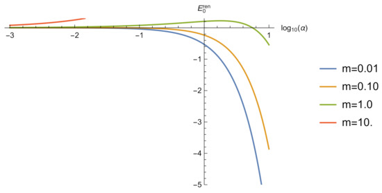
Figure 5.
The vacuum energy of a massive scalar field with repulsive self-interaction on the whole axis. All quantities are given in units of the mass .Spectrum
In the massless case the same remarks as in Section 3 apply. The vacuum energy is
The pole term for can be obtained either from the heat kernel coefficient , (65), and (44), or from inserting the asymptotic expansion (62) and it reads
Again, in the massless case we define the renormalized vacuum energy by subtracting the pole term,
Further we split
with, from the asymptotic expansion (62),
and the ’subtracted’ part,
where we could put . Finally, rearranging contributions gives us
with
This vacuum energy can now be calculated numerically. For technical reasons also the same splitting of as in Equation (74) was used. Examples are shown in Figure 6.
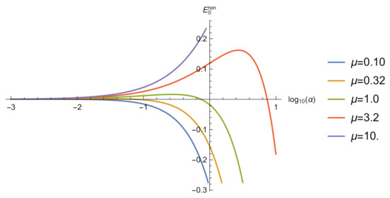
Figure 6.
The vacuum energy of a massless scalar field with repulsive self-interaction on the whole axis. and are given in units of .Spectrum
5. The Limit of Strong Coupling
In this section, we consider the limit , i.e., the limit of strong coupling in Equations (8) and (36), of the renormalized vacuum energy, which was calculated in the preceding two sections.
We start with the massive cases and equip the relevant energies with an index ‘1’ in place of the index ’0’ which mentions that this is a vacuum energy. For finite L, we have the energy (49) with its constituent parts (51) and (48). The subtracted energy (48) can be written in the form
Here, the function is the same as defined by (61). Before we can consider the limit , we need to rewrite the last term in the square bracket,
We get two terms. In the second,
we carry out the summation,
where is the harmonic number. In the limit we get
In the first term, for , the summation over j turns into an integration (similar to (57)) with
and we come to
Here, the integral gives a number and we introduce the notation
In the second line we made the substitution . This way, we get from (89)
Together with (56) we get from (49)
which is up to terms of zeroth order in .
Next we consider the massive case in infinite volume. We give it the index ‘3’. The asymptotic part of the energy is given by Equation (72) and we note
The subtracted part of the energy is given by Equation (69) and we note
The integrals over t can be brought into the form of the second line in (90),
and we arrive at
This is the same as (92).
We turn to the massless case and consider finite volume. This case gets the index ‘2’. The asymptotic part of the vacuum energy is given by (56) and takes in the limit the form
The subtracted part, (48), is, in this limit, the same as , (91), and for the renormalized energy we arrive
Finally, we have the case 4 which is infinite volume and massless field. The asymptotic part is given by Equation (82) and reads in the limit
The subtracted part, (80), is the same as in case 3 and reads
Taking these two together we arrive at
which is the same as (98), case 2.
As we have seen, the cases 1 and 3, as well as 2 and 4, have the same limit, which shows that this limit is independent on the volume. The massless cases, which depend on the arbitrary parameter , give the same as the massive cases with the formal substitution .
On the leading logarithmic behavior of the renormalized vacuum energy a more general view is possible. Let us consider the regularized vacuum energy, (37), for large . We represent the , (23), in the form
where we used the function , which was defined by (61). The regularized vacuum energy becomes
which is similar to (83). Now we consider the limit . The sum turns into an integration, following (88). The mass term disappears and we arrive at
where we made the substitution alike in (90). The integral is a function only of s. It has a pole in and the pole term is, of course, the same as in (44) (for ). This pole term generates the logarithmic contribution,
such that after subtracting the pole term, i.e., after preforming the renormalization, we get
The dots denote the terms without and depend on the renormalization scheme. Accounting for , (44) or (65), we reproduce the leading order in the above mentioned examples, (92), (96), (98) and (101).
6. Conclusions
We have calculated the vacuum energy for a scalar field with self-interaction in -dimensions in a box of length L with Dirichlet boundary conditions and in the whole space for both, massive and massless fields. For dimensional reasons, the vacuum energy has the following structure. We use the definition of the cases given in Section 5,
where the functions are dimensionless. These are shown in the figures in Section 3 and Section 4. We remind that for the infinite volume cases we consider the energy density.
The case 4 carries little new information. The vacuum energy (101) has only the factor in front of the logarithm as sensible information since the constant term remains undefined because of the arbitrary parameter . Further, the mentioned factor follows, for dimensional reasons, from the heat kernel coefficient , (65).
In the massive case, the renormalization is done by subtracting the contributions from the relevant heat kernel coefficients, which delivers a unique result. In distinction, in the massless case the arbitrary parameter remains present in the renormalized energy.
This way, we were able to attribute a sensible vacuum energy to a field with self-interaction in a flat and empty space. We underline that this result is not perturbative but calculated in all orders of the self-interaction.
A characteristic feature is the strong coupling behavior. It is calculated in Section 5 and shows in all four cases the same result of a growing negative vacuum energy. This allows for the interpretation that the vacuum energy makes the system unstable with respect to an increasing coupling. For smaller coupling, positive values are possible as can be seen from the figures. For vanishing coupling we reobtain the known result for a free field.
As only relation to a physical system we mention the relation to the dimensionless parameter introduced in [14], whose value in BEC experiments is , implying .
A final remark concerns the possible embedding of the vacuum energy calculated in this paper into some context. Obvious candidates would be the already mentioned BEC, where Equation (8) has the meaning of the Gross-Pitaevski equation, or an effective potential in the sense of Coleman-Weinberg. Since we were in the present paper only interested in the first calculation of vacuum energy for an interacting field, these questions are left for future work.
Funding
This research received no external funding.
Institutional Review Board Statement
Not applicable.
Informed Consent Statement
Not applicable.
Conflicts of Interest
The author declares no conflict of interest.
References
- Bordag, M.; Klimchitskaya, G.L.; Mohideen, U.; Mostepanenko, V.M. Advances in the Casimir Effect; Oxford University Press: Oxford, UK, 2009. [Google Scholar]
- Bordag, M. (Ed.) The Casimir Effect 50 Years Later. In Proceedings of the Fourth Workshop on Quantum Field Theory under the Influence of External Conditions, Leipzig, Germany, 14–18 September 1998; World Scientific: Singapore, 1999. [Google Scholar]
- Weinberg, S. The cosmological constant problem. Rev. Mod. Phys. 1989, 61, 1–23. [Google Scholar] [CrossRef]
- Mostepanenko, V.M.; Klimchitskaya, G.L. Whether an Enormously Large Energy Density of the Quantum Vacuum Is Catastrophic. Symmetry 2019, 11, 314. [Google Scholar] [CrossRef]
- Casimir, H.B.G. On the attraction between two perfectly conducting plates. Proc. Kon. Nederland. Akad. Wetensch 1948, 51, 793–795. [Google Scholar]
- Boyer, T. Quantum electromagnetic zero point energy of a conducting spherical shell and the Casimir model for a charged particle. Phys. Rev. D 1968, 14, 1764–1774. [Google Scholar] [CrossRef]
- Bordag, M.; Kirsten, K. Vacuum energy in a spherically symmetric background field. Phys. Rev. D 1996, 53, 5753–5760. [Google Scholar] [CrossRef] [PubMed]
- Ford, L. Casimir Effect for a Self-Interacting Scalar Field. Proc. R. Soc. Lond. A 1979, 368, 305–310. [Google Scholar] [CrossRef]
- Peterson, C.; Hansson, T.; Johnson:, K. Loop diagrams in boxes. Phys. Rev. D 1982, 26, 415. [Google Scholar] [CrossRef]
- Bordag, M.; Lindig, J. Radiative correction to the Casimir force on a sphere. Phys. Rev. D 1998, 58, 045003. [Google Scholar] [CrossRef]
- Valuyan, M.A. The Dirichlet Casimir energy for the ϕ4 theory in a rectangle. Eur. Phys. J. Plus 2018, 133, 401. [Google Scholar] [CrossRef]
- Song, P.T.; Thu, N.V. The Casimir Effect in a Weakly Interacting Bose Gas. J. Low Temp. Phys. 2021, 202, 160. [Google Scholar] [CrossRef]
- Dashen, R.F.; Hasslacher, B.; Neveu, A. Semiclassical bound states in an asymptotically free theory. Phys. Rev. D 1975, 12, 2443–2458. [Google Scholar] [CrossRef]
- Carr, L.D.; Clark, C.W.; Reinhardt, W.P. Stationary solutions of the one-dimensional nonlinear Schrödinger equation. I. Case of repulsive nonlinearity. Phys. Rev. A 2000, 62, 063610. [Google Scholar] [CrossRef]
- Carr, L.D.; Clark, C.W.; Reinhardt, W.P. Stationary solutions of the one-dimensional nonlinear Schrödinger equation. II. Case of attractive nonlinearity. Phys. Rev. A 2000, 62, 063611. [Google Scholar] [CrossRef]
- Espichán Carrillo, J.A.; Maia, A., Jr.; Mostepanenko, V.M. Jacobi elliptic solutions of λϕ4 theory in a finite domain. Int. J. Mod. Phys. A 2000, 15, 2645–2659. [Google Scholar] [CrossRef]
- Sacchetti, A. Stationary solutions to cubic nonlinear Schrödinger equations with quasi-periodic boundary conditions. J. Phys. A Math. Theor. 2020, 53, 385204. [Google Scholar] [CrossRef]
- Olver, F.; Lozier, D.; Boisvert, R.; Clark, C. NIST Handbook of Mathematical Functions: With Formulas, Graphs, and Mathematical Tables; Cambridge University Press: Cambridge, UK, 2010. [Google Scholar]
- Seaman, B.T.; Carr, L.D.; Holland, M.J. Nonlinear band structure in Bose–Einstein condensates: Nonlinear Schrödinger equation with a Kronig-Penney potential. Phys. Rev. A 2005, 71, 033622. [Google Scholar] [CrossRef]
- Gradshteyn, I.; Ryzhik, I. Table of Integrals, Series and Products; Academic Press: New York, NY, USA, 2007. [Google Scholar]
- Bordag, M.; Pirozhenko, I.G. The closed piecewise uniform string revisited. arXiv 2020, arXiv:hep-th/2012.14301. [Google Scholar]


Publisher’s Note: MDPI stays neutral with regard to jurisdictional claims in published maps and institutional affiliations. |
© 2021 by the author. Licensee MDPI, Basel, Switzerland. This article is an open access article distributed under the terms and conditions of the Creative Commons Attribution (CC BY) license (http://creativecommons.org/licenses/by/4.0/).