
Quantum Cosmology with Third Quantisation


Abstract
| Contents | ||||
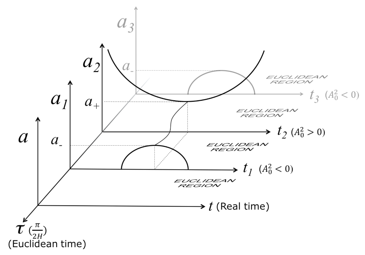
| 1 | Introduction . . . . . . . . . . . . . . . . . . . . . . . . . . . . . . . . . . . . . . . . . . . . . . . . . . . . . . . . . . . . . . . . . . . . | 2 | ||
| 2 | Quantisation of a Simply Connected Spacetime Manifold . . . . . . . . . . . . . . . . . . . . . . . . . . . . . . | 3 | ||
| 2.1 | Quantisation of the Spacetime Geometry . . . . . . . . . . . . . . . . . . . . . . . . . . . . . . . . . . . . . . . . | 3 | ||
| 2.2 | Boundary Conditions . . . . . . . . . . . . . . . . . . . . . . . . . . . . . . . . . . . . . . . . . . . . . . . . . . . . . . . . | 7 | ||
| 2.3 | Semiclassical Quantum Gravity . . . . . . . . . . . . . . . . . . . . . . . . . . . . . . . . . . . . . . . . . . . . . . . | 9 | ||
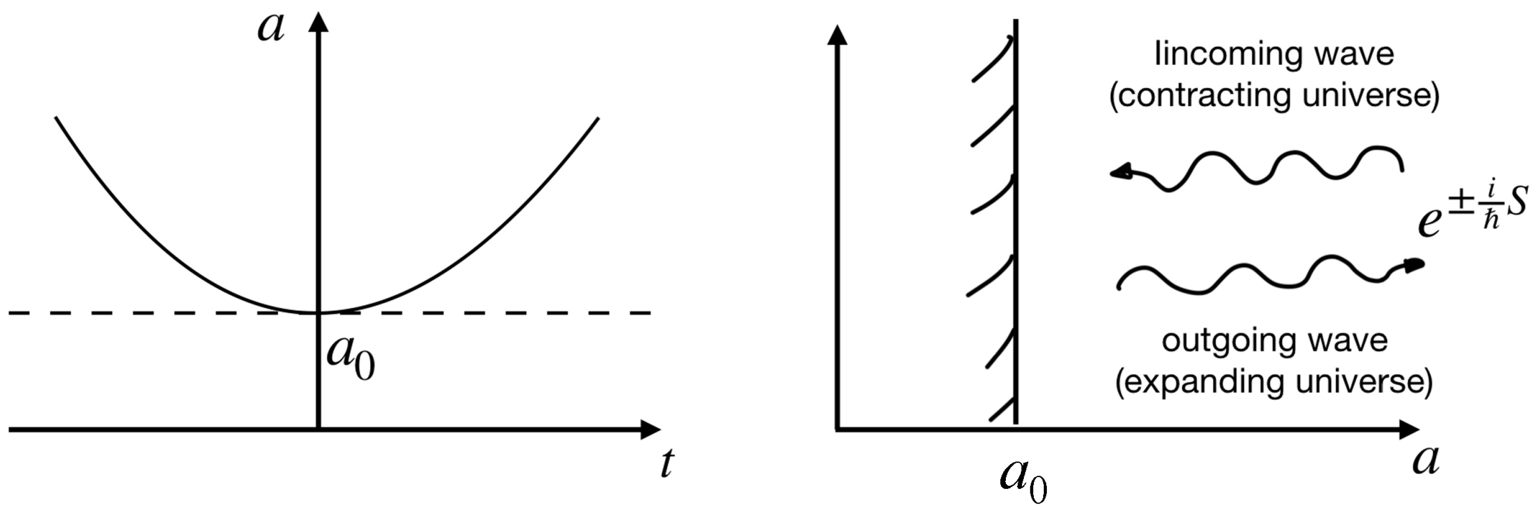
| 2.4 | Minisuperspace Model . . . . . . . . . . . . . . . . . . . . . . . . . . . . . . . . . . . . . . . . . . . . . . . . . . . . . . | 11 | ||
| 2.4.1 | Inflationary Universe . . . . . . . . . . . . . . . . . . . . . . . . . . . . . . . . . . . . . . . . . . . . . . . . . | 13 | ||
| 2.4.2 | Small Perturbations and Backreaction . . . . . . . . . . . . . . . . . . . . . . . . . . . . . . . . . . . | 15 | ||
| 2.5 | Paradigms for the Creation of the Universe in Quantum Cosmology . . . . . . . . . . . . . . . . | 20 | ||
| 2.5.1 | Creation of the Universe from Nothing . . . . . . . . . . . . . . . . . . . . . . . . . . . . . . . . . . . | 22 | ||
| 2.5.2 | Creation of the Universe from Something . . . . . . . . . . . . . . . . . . . . . . . . . . . . . . . . . | 26 | ||
| 2.5.3 | Creation of Universes in Pairs . . . . . . . . . . . . . . . . . . . . . . . . . . . . . . . . . . . . . . . . . . | 28 | ||
| 3 | Third Quantisation Formalism . . . . . . . . . . . . . . . . . . . . . . . . . . . . . . . . . . . . . . . . . . . . . . . . . . . . | 29 | ||
| 3.1 | Historial Review . . . . . . . . . . . . . . . . . . . . . . . . . . . . . . . . . . . . . . . . . . . . . . . . . . . . . . . . . . . . | 29 | ||
| 3.2 | Quantum Field Theory in M ≡ Riem(Σ) . . . . . . . . . . . . . . . . . . . . . . . . . . . . . . . . . . . . . . . . . | 33 | ||
| 3.2.1 | Geometrical Structure of M . . . . . . . . . . . . . . . . . . . . . . . . . . . . . . . . . . . . . . . . . . . . | 33 | ||
| 3.2.2 | Classical Evolution of the Universe . . . . . . . . . . . . . . . . . . . . . . . . . . . . . . . . . . . . . | 35 | ||
| 3.2.3 | Quantum Field Theory in M . . . . . . . . . . . . . . . . . . . . . . . . . . . . . . . . . . . . . . . . . . . | 36 | ||
| 3.2.4 | Boundary Conditions and the Creation of the Universes in Pairs . . . . . . . . . . . . . | 39 | ||
| 3.2.5 | Semiclassical Regime . . . . . . . . . . . . . . . . . . . . . . . . . . . . . . . . . . . . . . . . . . . . . . . . . . | 41 | ||
| 3.3 | Minisuperspace Model . . . . . . . . . . . . . . . . . . . . . . . . . . . . . . . . . . . . . . . . . . . . . . . . . . . . . . | 43 | ||
| 3.3.1 | Geometrical Structure of the Minisuperspace . . . . . . . . . . . . . . . . . . . . . . . . . . . . . | 43 | ||
| 3.3.2 | Field Quantisation of a FRW Spacetime . . . . . . . . . . . . . . . . . . . . . . . . . . . . . . . . . . | 47 | ||
| 3.3.3 | Reheating and the Matter–Antimatter Content of the Entangled Universe . . . . . | 49 | ||
| 4 | Observable Effects of Quantum Cosmology . . . . . . . . . . . . . . . . . . . . . . . . . . . . . . . . . . . . . . . . . | 54 | ||
| 5 | Conclusions . . . . . . . . . . . . . . . . . . . . . . . . . . . . . . . . . . . . . . . . . . . . . . . . . . . . . . . . . . . . . . . . . . . . | 56 | ||
| References . . . . . . . . . . . . . . . . . . . . . . . . . . . . . . . . . . . . . . . . . . . . . . . . . . . . . . . . . . . . . . . . . . . . . . . . . | 60 | |||
1. Introduction
2. Quantisation of a Simply Connected Spacetime Manifold
2.1. Quantisation of the Spacetime Geometry


2.2. Boundary Conditions
2.3. Semiclassical Quantum Gravity
2.4. Minisuperspace Model
2.4.1. Inflationary Universe
2.4.2. Small Perturbations and Backreaction
2.5. Paradigms for the Creation of the Universe in Quantum Cosmology
2.5.1. Creation of the Universe from Nothing
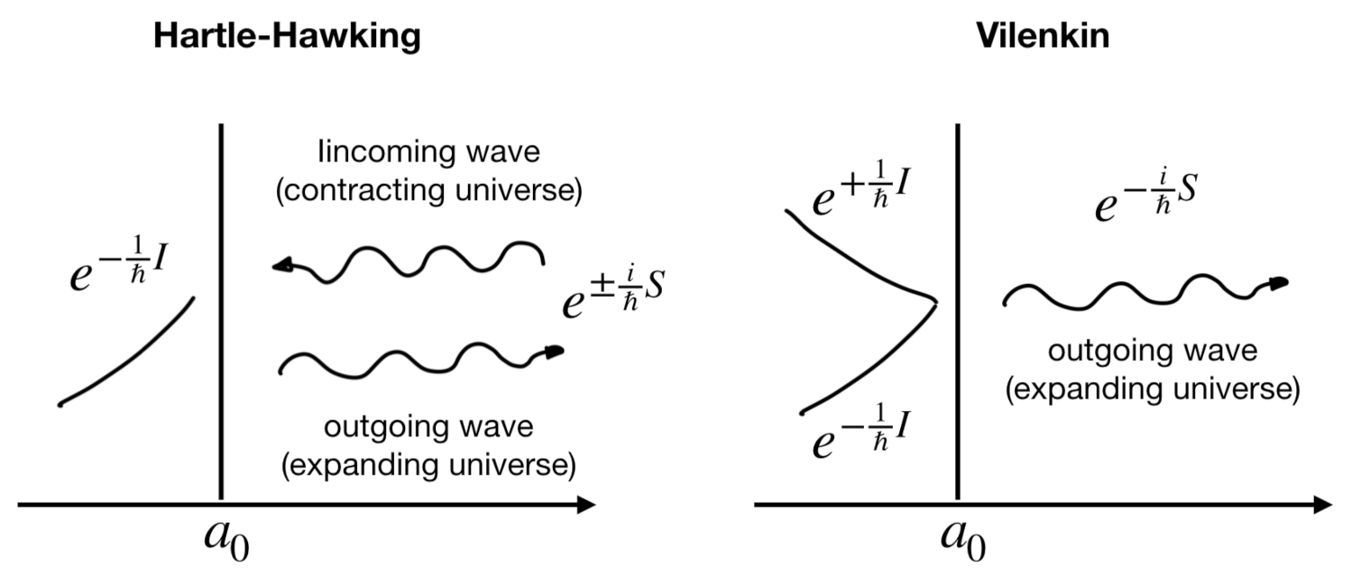
Vilenkin’s vs. Hartle–Hawking’s Versions
2.5.2. Creation of the Universe from Something
Gott and Li: The Universe Is Its Own Mother
2.5.3. Creation of Universes in Pairs
3. Third Quantisation Formalism
3.1. Historial Review
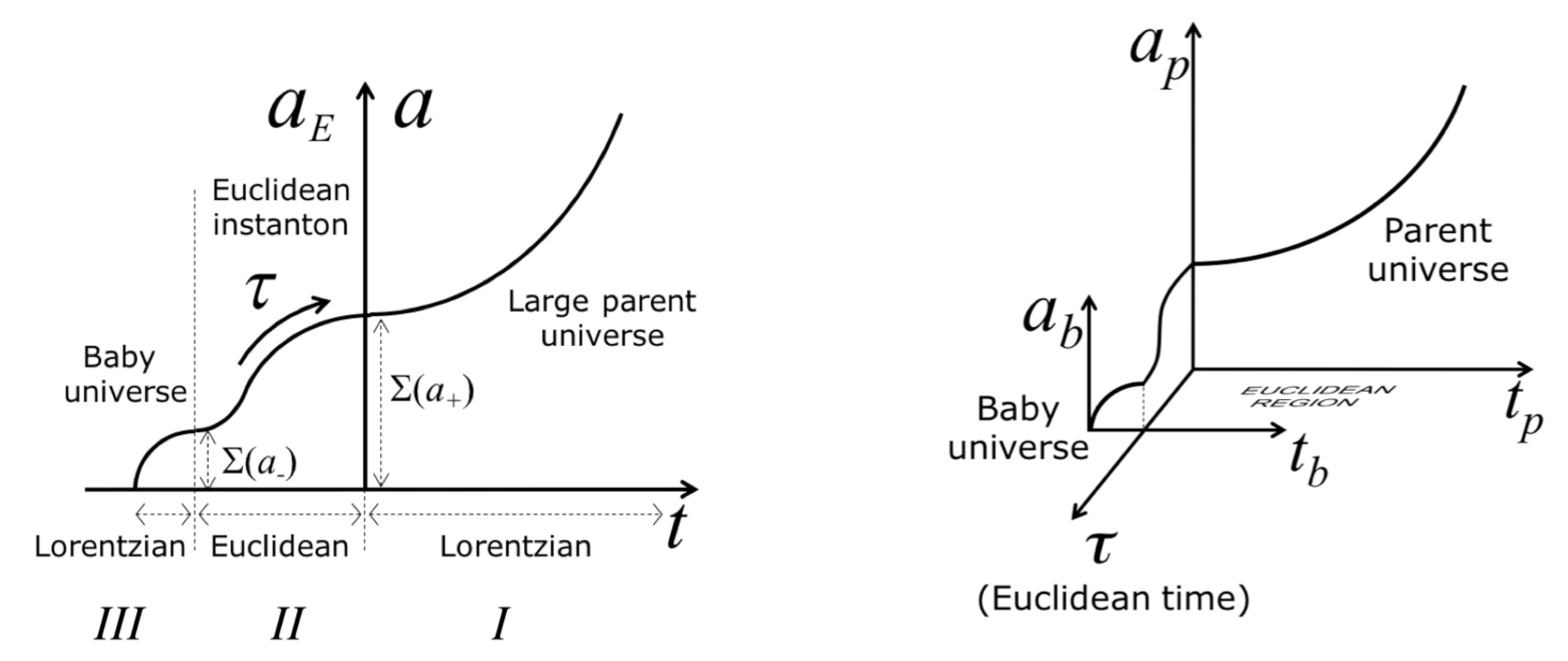
Parent and Baby Universes: The Hybrid Action
3.2. Quantum Field Theory in
3.2.1. Geometrical Structure of M
3.2.2. Classical Evolution of the Universe
3.2.3. Quantum Field Theory in M
3.2.4. Boundary Conditions and the Creation of the Universes in Pairs
3.2.5. Semiclassical Regime
3.3. Minisuperspace Model
3.3.1. Geometrical Structure of the Minisuperspace
3.3.2. Field Quantisation of a FRW Spacetime
3.3.3. Reheating and the Matter–Antimatter Content of the Entangled Universe
4. Observable Effects of Quantum Cosmology
5. Conclusions
Funding
Acknowledgments
Conflicts of Interest
| 1 | |
| 2 | More exactly, it is isomorphic to a Milne spacetime, which is a particular coordination of the light cones of the Minkowski spacetime. |
| 3 | |
| 4 | Following Ref. [10], we are going to use throughout units in which, , although we will leave the constant ℏ in some expressions to remark their quantum character. |
| 5 | For the matter fields we shall generally consider a scalar field. |
| 6 | We shall be more precise later on. |
| 7 | Spacetime becomes a ’trajectory of spaces’, cfr. p. 107, Ref. [7]. |
| 8 | Let us assume that the period of inflation is fully supported by the current observational data. |
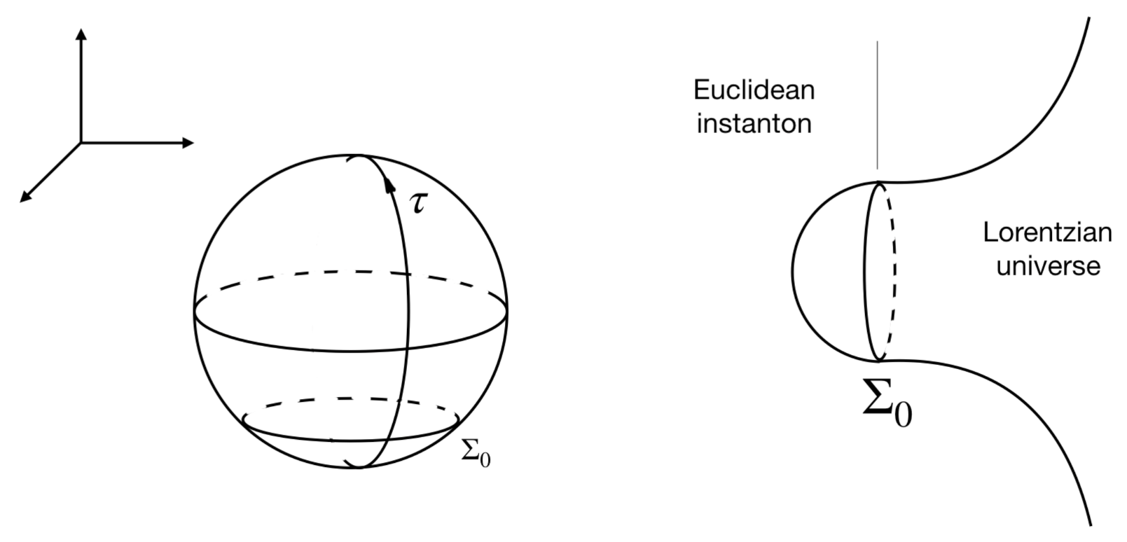
| 9 | Let us notice however that the creation of this initial boundary hypersurface is not a process occurring in time but it corresponds to the creation of the spacetime itself [7], actually. |
| 10 | |
| 11 | A classical path of the superspace is invariant under reparametrisations so by time we mean any time variable. |
| 12 | For instance, the march of a material clock would be given by the matter fields that are solutions of Einstein’s equations, in a circular argument. |
| 13 | Sometimes it is distinguished between minisuperspace and midisuperspace models depending on the number of variables of the reduced superspace. |
| 14 | |
| 15 | Unless otherwise indicated we shall always use cosmic time, t, for which . |
| 16 | Recall that after doing the variation with respect to N we can fix any particular value. |
| 17 | However, one would generally expect that the creation of the universe comes from a quantum fluctuation of the spacetime and therefore be of order of the Planck scale, . In that case, new elements should be incorporated, although the picture described here and in the next section would still be instructive. |
| 18 | This is especially clear in the case of the cosmic microwave background radiation (CMB), in which the relative scale of the energy fluctuations in the last scattering surface are of order . |
| 19 | By ’matter degrees of freedom’ we mean the perturbation modes that can represent matter, radiation or even fluctuations of the gravitational field (gravitons). |
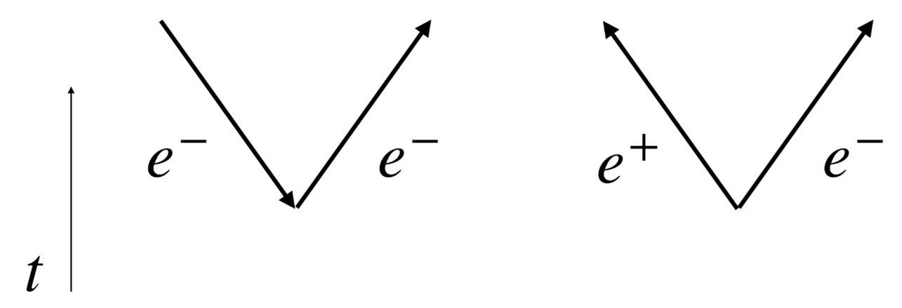
| 20 | In terms of we would have ended up with two contracting universes, one made of matter and the other made up of antimatter. However, that case is not interesting because the two newborn contracting universes would rapidly delve into the spacetime foam from which they came up |
| 21 | Here, the field is the Schrödinger wave function . |
| 22 | In Ref. [29] it is shown that the distribution of a large number harmonic oscillators becomes highly peaked around its average value. |
| 23 | Let us note however that this is only a formal analogy. In fact, the Hamiltonian constraint (89) indicates is that the total energy of the universe is zero, i.e., the (negative) energy of the spacetime exactly balances the (positive) energy of the matter fields. |
| 24 | Let us note however that this process does not violate the conservation of the energy because the total energy, i.e., the gravitational energy plus the energy of the matter fields is, as we have already said, balanced. |
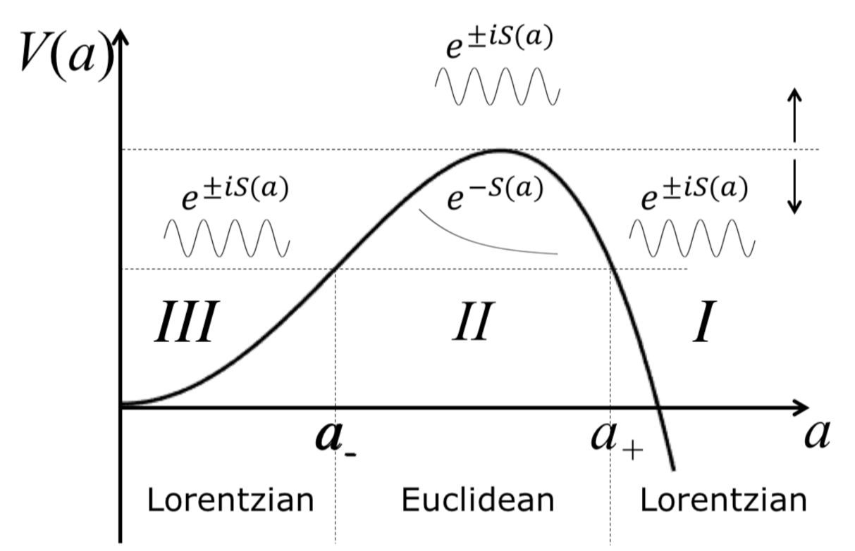
| 25 | These are the final values of the Euclidean regime. From the point of view of the Lorentzian sections, these are the “initial” values. |
| 26 | As we have seen, it is somehow arbitrary determining which solution describes an expanding universe and accordingly there is an ambiguity in determining which modes are the ’outgoing’ modes. |
| 27 | In Section 3.3 we shall define more concretely the operator ∇ in the minisuperspace. |
| 28 | In the superposition (127) it should appear , with . However, the eigenfunctions of the harmonic oscillator are real functions so, . |
| 29 | In general, a non simply connected manifold can be divided into N simply connected parts [59] and this N parts can be seen as N classically independent universes. |
| 30 | Typically, large regions of order of the Hubble length of our universe. |
| 31 | In the 1980s–1990s, the paradigm was a universe in a non-accelerated expansion. |
| 32 | It means that the state (146) would actually be,
|
| 33 | We have followed the normalisation applied in Ref. [10]. |
| 34 | |
| 35 | For the Milne spacetime, see Ref. [64] |
| 36 | A rescale, , , …, has been made to absorb the constant a. |
| 37 | Assuming the value, . |
| 38 | The fact that the trajectory is not a geodesic is not really determinant. In fact, using a generalisation of the Maupertuis principle [65,66], one can compute the metric where the trajectory of the universe is a geodesic. Let us consider the reparametrisation given by, and . In that case, the action (162) turns out to be
|
| 39 | For a FRW spacetime, (because, ). |
| 40 | |
| 41 | Let us notice that the condition, , does not assume that the universe is homogeneous. |
| 42 | The factor has been introduced for later convenience. |
| 43 | In the 2 sphere, . |
| 44 | |
| 45 | We are considering geometrically closed spatial sections. |
| 46 | The inhomogeneities of the spacetime can also be considered as fields propagating in the spacetime (see Section 2). |
| 47 | A similar procedure can be followed in a curved spacetime. |
| 48 | We shall use now the variable to represent the inflaton field and leave the variable to represent collectively the rest of fields of the SM. |
| 49 | Although other mechanisms of baryon asymmetry can simultaneously be present. |
| 50 | Typically, would represent a linear combination of the and fields. In that case, would represent the corresponding conjugated combination. |
| 51 | Tegmark poses the following example: a theory stating that there are 666 parallel universes, all of which are devoid of oxygen, makes the testable prediction that we should observe no oxygen here, and is therefore ruled out by observation, cfr. Ref. [97], p. 105. |
| 52 |
References
- Wheeler, J.A. On the nature of quantum geometrodynamics. Ann. Phys. 1957, 2, 604–614. [Google Scholar] [CrossRef]
- Gell-Mann, M.; Hartle, J.B. Quantum mechanics in the light of quantum cosmology. In Complexity, Entropy and the Physics of Information; Zurek, W.H., Ed.; Addison-Wesley: Reading, PA, USA, 1990. [Google Scholar]
- Halliwell, J.J. Decoherence in quantum cosmology. Phys. Rev. D 1989, 39, 2912–2923. [Google Scholar] [CrossRef] [PubMed]
- Kiefer, C. Decoherence in quantum electrodynamics and quantum gravity. Phys. Rev. D 1992, 46, 1658–1670. [Google Scholar] [CrossRef] [PubMed]
- Hartle, J.B. The quantum mechanics of cosmology. In Quantum Cosmology and Baby Universes; Coleman, S., Hartle, J.B., Piran, T., Weinberg, S., Eds.; World Scientific: London, UK, 1990; Volume 7. [Google Scholar]
- Kiefer, C. Continuous measurement of mini-superspace variables by higher multipoles. Class. Quant. Grav. 1987, 4, 1369–1382. [Google Scholar] [CrossRef]
- Kiefer, C. Quantum Gravity; Oxford University Press: Oxford, UK, 2007. [Google Scholar]
- Wiltshire, D.L. An Introduction to Quantum Cosmology. In Cosmology: The Physics of the Universe; Robson, B., Visvanathan, N., Woolcock, W., Eds.; World Scientific: Singapore, 1996; pp. 473–531. [Google Scholar]
- Wheeler, J.A. Superspace and the nature of quantum geometrodynamics. In Battelle Rencontres; DeWitt, C.M., Wheeler, J.A., Eds.; W. A. Benjamin, Inc.: New York, NY, USA, 1968; Chapter 9. [Google Scholar]
- De Witt, B.S. Quantum Theory of Gravity. I. The Canonical Theory. Phys. Rev. 1967, 160, 1113–1148. [Google Scholar] [CrossRef]
- Dirac, P.A.M. Lectures on Quantum Mechanics. In Belfer Graduate School of Science Monographs Series; Number 2; Belfer Graduate School of Science: New York, NY, USA, 1964. [Google Scholar]
- Hartle, J.B.; Hawking, S.W. Wave function of the Universe. Phys. Rev. D 1983, 28, 2960. [Google Scholar] [CrossRef]
- Joos, E.; Zeh, H.D.; Kiefer, C.; Giulini, D.J.; Kupsch, J.; Stamatescu, I.O. Decoherence and the Appearance of a Classical World in Quantum Theory; Springer: Berlin, Germany, 2003. [Google Scholar]
- Schlosshauer, M. Decoherence and the Quantum-to-Classical Transition; Springer: Berlin, Germany, 2007. [Google Scholar]
- Halliwell, J.J. Introductory lectures on quantum cosmology. In Quantum Cosmology and Baby Universes; Coleman, S., Hartle, J.B., Piran, T., Weinberg, S., Eds.; World Scientific: London, UK, 1990; Volume 7. [Google Scholar]
- Davidson, A.; Ygael, T. From DeWitt initial condition to cosmological quantum entanglement. Class. Quant. Grav. 2015, 32, 152001. [Google Scholar] [CrossRef][Green Version]
- Kiefer, C.; Singh, T.P. Quantum gravitational corrections to the functional Schrödinger equation. Phys. Rev. D 1991, 44, 1067. [Google Scholar] [CrossRef]
- Kiefer, C.; Krämer, M. Quantum gravitational contributions to the CMB anisotropy spectrum. Phys. Rev. Lett. 2012, 108, 021301. [Google Scholar] [CrossRef]
- Brizuela, D.; Kiefer, C.; Krämer, M. Quantum-gravitational effects on gauge-invariant scalar and tensor perturbations during inflation: The de Sitter case. Phys. Rev. D 2016, 93, 104035. [Google Scholar] [CrossRef]
- Brizuela, D.; Kiefer, C.; Krämer, M. Quantum-gravitational effects on gauge-invariant scalar and tensor perturbations during inflation: The slow-roll approximation. Phys. Rev. D 2016, 94, 123527. [Google Scholar] [CrossRef]
- Hartle, J.B. Spacetime quantum mechanics and the quantum mechanics of spacetime. arXiv 1995, arXiv:gr-qc/9304006. [Google Scholar]
- Bezrukov, F.L.; Shaposhnikov, M.E. The Standard Model Higgs boson as the inflaton. Phys. Lett. B 2008, 659, 703. [Google Scholar] [CrossRef]
- Garcia-Bellido, J.; Figueroa, D.G.; Rubio, J. Preheating in the Standard Model with the Higgs-Inflaton coupled to gravity. Phys. Rev. D 2009, 79, 063531. [Google Scholar] [CrossRef]
- Garay, I.; Robles-Pérez, S. Effects of a scalar field on the thermodynamics of interuniversal entanglement. Int. J. Mod. Phys. D 2014, 23, 1450043. [Google Scholar] [CrossRef]
- Linde, A. Particle Physics and Inflationary Cosmology; Contemporary Concepts in Physics; Harwood Academic Publishers: Chur, Switzerland, 1993; Volume 5. [Google Scholar]
- Rubakov, V.A. Quantum Cosmology. In Lecture at NATO ASI ‘Structure Formation in the Universe’; Springer: Cambridge, MA, USA, 1999. [Google Scholar]
- Halliwell, J.J.; Hawking, S.W. Origin of structure in the Universe. Phys. Rev. D 1985, 31, 1777–1791. [Google Scholar] [CrossRef] [PubMed]
- Rubakov, V.A. On third quantization and the cosmological constant. Phys. Lett. B 1988, 214, 503–507. [Google Scholar] [CrossRef]
- Halliwell, J.J. Correlations in the wave function of the Universe. Phys. Rev. D 1987, 36, 3626–3640. [Google Scholar] [CrossRef]
- Grishchuk, L.P.; Sidorov, Y.V. Squeezed quantum states of relic gravitons and primordial density fluctuations. Phys. Rev. D 1990, 42, 3413–3421. [Google Scholar] [CrossRef]
- Lewis, H.R.; Riesenfeld, W.B. An Exact Quantum THeory of the Time-Dependent Harmonic Oscillator and of a Charged Particle in a Time-Dependent Electromagnetic Field. J. Math. Phys. 1969, 10, 1458–1473. [Google Scholar] [CrossRef]
- Leach, P.G.L. Harmonic oscillator with variable mass. J. Phys. A 1983, 16, 3261–3269. [Google Scholar] [CrossRef]
- Kanasugui, H.; Okada, H. Systematic treatments of general time-dependent harmonica oscillator in classical and quantum mechanics. Prog. Theor. Phys. 1995, 93, 949–960. [Google Scholar] [CrossRef]
- Sheng, D.; Khan, R.D.; Jialun, Z.; Wenda, S. Quantum Harmonic Oscillator with Time-Dependent Mass and Frequency. Int. J. Theor. Phys. 1995, 34, 355–368. [Google Scholar] [CrossRef]
- Brizuela, D.; Kiefer, C.; Krämer, M.; Robles-Pérez, S. Quantum-gravity effects for excited states of inflationary perturbations. Phys. Rev. D 2019, 99, 104007. [Google Scholar] [CrossRef]
- Robles-Pérez, S. Quantum cosmology of a conformal multiverse. Phys. Rev. D 2017, 96, 063511. [Google Scholar] [CrossRef]
- Hawking, S.W. The boundary conditions of the universe. In Astrophysical Cosmology; Pontificia Academiae Scientarium: Vatican City, Vatican, 1982; pp. 563–572. [Google Scholar]
- Hawking, S.W. Quantum cosmology. In Relativity, groups and topology II, Les Houches, Session XL, 1983; De Witt, B.S., Stora, R., Eds.; Elsevier Science Publishers B.V.: Amsterdam, The Netherlands, 1984. [Google Scholar]
- Hawking, S.W. The quantum state of the universe. Nucl. Phys. B 1984, 239, 257–276. [Google Scholar] [CrossRef]
- Vilenkin, A. Creation of universes from nothing. Phys. Lett. B 1982, 117, 25–28. [Google Scholar] [CrossRef]
- Vilenkin, A. Quantum creation of universes. Phys. Rev. D 1984, 30, 509–511. [Google Scholar] [CrossRef]
- Vilenkin, A. Boundary conditions in quantum cosmology. Phys. Rev. D 1986, 33, 3560–3569. [Google Scholar] [CrossRef]
- Vilenkin, A. Predictions from Quantum Cosmology. Phys. Rev. Lett. 1995, 74, 846–849. [Google Scholar] [CrossRef] [PubMed]
- Vilenkin, A. Interpretation of the wave function of the universe. Phys. Rev. D 1989, D, 1116. [Google Scholar] [CrossRef] [PubMed]
- Gott, J.R.I.; Li, L.X. Can the universe create itself? Phys. Rev. D 1998, 58, 023501. [Google Scholar] [CrossRef]
- Strominger, A. Baby Universes. In Quantum Cosmology and Baby Universes; Coleman, S., Hartle, J.B., Piran, T., Weinberg, S., Eds.; World Scientific: London, UK, 1990; Volume 7. [Google Scholar]
- Barvinsky, A.O.; Kamenshchik, A.Y. Cosmological Landscape From Nothing: Some Like It Hot. JCAP 2006, 0609, 014. [Google Scholar] [CrossRef]
- Barvinsky, A.O.; Kamenshchik, A.Y. Cosmological landscape and Euclidean quantum gravity. J. Phys. A 2007, 40, 7043–7048. [Google Scholar] [CrossRef][Green Version]
- Barvinsky, A.O. Why there is something rather than nothing (out of everything)? Phys. Rev. Lett. 2007, 99, 071301. [Google Scholar] [CrossRef]
- Robles-Pérez, S.; González-Díaz, P.F. Quantum entanglement in the multiverse. JETP 2014, 118, 34. [Google Scholar] [CrossRef]
- Robles-Pérez, S.J. Creation of entangled universes avoids the Big Bang singularity. J. Gravity 2014, 2014, 382675. [Google Scholar] [CrossRef]
- Chen, P.; Hu, Y.C.; Yeom, D.H. Fuzzy Euclidean wormholes in de Sitter space. JCAP 2017, 07, 001. [Google Scholar] [CrossRef]
- Caderni, N.; Martellini, M. Third quantization formalism for Hamiltonian cosmologies. Int. J. Theor. Phys. 1984, 23, 233. [Google Scholar] [CrossRef]
- Coleman, S. Black holes as red herrings: Topological fluctuations and the loss of quantum coherence. Nucl. Phys. B 1988, 307, 867. [Google Scholar] [CrossRef]
- Coleman, S. Why there is nothing rather than something? A theory of the cosmological constant. Nucl. Phys. B 1988, 310, 643–668. [Google Scholar] [CrossRef]
- McGuigan, M. Third quantization and the Wheeler-DeWitt equation. Phys. Rev. D 1988, 38, 3031. [Google Scholar] [CrossRef] [PubMed]
- McGuigan, M. Universe creation from the third quantized vacuum. Phys. Rev. D 1989, 39, 2229. [Google Scholar] [CrossRef] [PubMed]
- McGuigan, M. Universe decay and changing the cosmological constant. Phys. Rev. D 1990, 41, 418. [Google Scholar] [CrossRef] [PubMed]
- Hawking, S.W. Wormholes and Non-simply Connected Manifolds. In Quantum Cosmology and Baby Universes; Coleman, S., Hartle, J.B., Piran, T., Weinberg, S., Eds.; World Scientific: London, UK, 1990; Volume 7. [Google Scholar]
- González-Díaz, P.F. Nonclassical states in quantum gravity. Phys. Lett. B 1992, 293, 294. [Google Scholar] [CrossRef]
- González-Díaz, P.F. Regaining quantum incoherence for matter fields. Phys. Rev. D 1992, 45, 499. [Google Scholar] [CrossRef]
- Higuchi, A.; Wald, R.M. Applications of a new proposal for solving the problem of time to some simple quantum cosmological models. Phys. Rev. D 1995, 51, 544–561. [Google Scholar] [CrossRef] [PubMed]
- Barbour, J. Shape Dynamics. An introduction. In Quantum Field Theory and Gravity; Finster, F., Müller, O., Nardmann, M., Tolksdorf, J., Zeidler, E., Eds.; Springer: Basel, Switerland, 2012; pp. 257–297. [Google Scholar]
- Griffiths, J.B.; Podolsky, J. Exact Space-Times in Einstein’s General Relativity; Cambridge Monographs on Mathematical Physics; Cambridge University Press: Cambridge, UK, 2009. [Google Scholar]
- Biesiada, M.; Rugh, S. Maupertuis principle, Wheeler’s superspace and an invariant criterion for local instability in general relativity. arXiv 1994, arXiv:gr-qc/9408030. [Google Scholar]
- Garay, I.; Robles-Pérez, S. Classical geodesics from the canonical quantisation of spacetime coordinates. arXiv 2019, arXiv:1901.05171. [Google Scholar]
- Pimentel, L.O.; Mora, C. Third quantization of Brans-Dicke Cosmology. Phys. Lett. A 2001, 280, 191–196. [Google Scholar] [CrossRef]
- Kim, S.P. Third quantization and quantum universes. arXiv 2012, arXiv:1212.535. [Google Scholar] [CrossRef]
- Ohkuwa, Y.; Ezawa, Y. Third quantization of f(R)-type gravity II—General f(R) case. Class. Quantum Gravity 2013, 20, 235015. [Google Scholar] [CrossRef]
- Calgani, G.; Gielen, S.; Oriti, D. Group field theory cosmology: A cosmological field theory of quantum geometry. Class. Quantum Gravity 2012, 29, 105005. [Google Scholar] [CrossRef]
- Faizal, M. Multiverse in the third quantized formalism. Commun. Theor. Phys. 2014, 62, 697. [Google Scholar] [CrossRef][Green Version]
- Balcerzak, A.; Marosek, K. Emergence of multiverse in third quantized varying constants cosmologies. Eur. Phys. J. C 2019, 79, 563. [Google Scholar] [CrossRef]
- Balcerzak, A.; Marosek, K. Doubleverse entanglement in third quantized non-minimally coupled varying constants cosmologies. Eur. Phys. J. C 2020, 80, 709. [Google Scholar] [CrossRef]
- Campanelli, L. Creation of universes from the third-quantized vacuum. Phys. Rev. D 2020, 102, 043514. [Google Scholar] [CrossRef]
- Robles-Pérez, S.J. Hartle-Hawking vacuum is full of Vilenkin’s universe-antiuniverse pairs. arXiv 2021, arXiv:2110.06521. [Google Scholar]
- Birrell, N.D.; Davies, P.C.W. Quantum Fields in Curved Space; Cambridge University Press: Cambridge, UK, 1982. [Google Scholar]
- Mukhanov, V.F.; Winitzki, S. Quantum Effects in Gravity; Cambridge University Press: Cambridge, UK, 2007. [Google Scholar]
- Bander, M.; Itzykson, C. Group theory and the hydrogen atom (II). Rev. Mod. Phys. 1966, 38, 346. [Google Scholar] [CrossRef]
- Lewis, H.R. Class of exact invariants for classical and quantum time dependent harmonic oscillators. J. Math. Phys. 1968, 9, 1976. [Google Scholar] [CrossRef]
- Pedrosa, I.A. Comment on “Coherent states for the time-dependent harmonic oscillator”. Phys. Rev. D 1987, 36, 1279. [Google Scholar] [CrossRef]
- Dantas, C.M.A.; Pedrosa, I.A.; Baseia, B. Harmonic oscillator with time-dependent mass and frequency and a perturbative potential. Phys. Rev. A 1992, 45, 1320. [Google Scholar] [CrossRef]
- Song, D.Y. Unitary relation between a harmonic oscillator of time-dependent frequency and a simple harmonic oscillator with and withuot an inverse-square potential. Phys. Rev. A 2000, 62, 014103. [Google Scholar] [CrossRef]
- Kim, S.P.; Page, D.N. Classical and quantum action-phase variables for time-dependent oscillators. Phys. Rev. A 2001, 64, 012104. [Google Scholar] [CrossRef]
- Park, T.J. Canonical Transformations for Time-Dependent Harmonic Oscillators. Bull. Korean Chem. Soc. 2004, 25. [Google Scholar]
- Robles-Pérez, S. Invariant vacuum. Phys. Lett. B 2017, 774, 608–615. [Google Scholar] [CrossRef]
- Rajeev, K.; Chakraborty, S.; Padmanabhan, T. Inverting a normal harmonic oscillator: Physical interpretation and applications. Gen. Rel. Grav. 2018, 50, 116. [Google Scholar] [CrossRef]
- Olson, S.J.; Ralph, T.C. Entanglement between the future and past in the quantum vacuum. Phys. Rev. Lett. 2011, 106, 110404. [Google Scholar] [CrossRef] [PubMed]
- Feynman, R.P. The theory of positrons. Phys. Rev. 1949, 76, 749. [Google Scholar] [CrossRef]
- Robles-Pérez, S.J. Cosmological perturbations in the entangled inflationary universe. Phys. Rev. D 2018, 97, 066018. [Google Scholar] [CrossRef]
- Robles-Pérez, S.J. Time reversal symmetry in cosmology and the creation of a universe-antiuniverse pair. Universe 2019, 5, 150. [Google Scholar] [CrossRef]
- Robles-Pérez, S.J. Restoration of matter-antimatter symmetry in the multiverse. arXiv 2017, arXiv:1706.06304. [Google Scholar]
- Robles-Pérez, S.J. Quantum cosmology in the light of quantum mechanics. Galaxies 2019, 7, 50. [Google Scholar] [CrossRef]
- Robles-Pérez, S.; González-Díaz, P.F. Quantum state of the multiverse. Phys. Rev. D 2010, 81, 083529. [Google Scholar] [CrossRef]
- Mukhanov, V.F. Physical Foundations of Cosmology; Cambridge University Press: Cambridge, UK, 2008. [Google Scholar]
- Kofman, L.; Linde, A.; Starobinsky, A.A. Towards the theory of reheating after inflation. Phys. Rev. D 1997, 56, 3258. [Google Scholar] [CrossRef]
- Boyle, L.; Finn, K.; Turok, N. CPT-Symmetric universe. Phys. Rev. Lett. 2018, 121, 251301. [Google Scholar] [CrossRef] [PubMed]
- Tegmark, M. The multiverse hierarchy. In Universe or Multiverse; Carr, B., Ed.; Cambridge University Press: Cambridge, UK, 2007; Chapter 7. [Google Scholar]
- Alonso-Serrano, A.; Jannes, G. Conceptual challenges on the road to the multiverse. Universe 2019, 5, 212. [Google Scholar] [CrossRef]
- Scardigli, F.; Gruber, C.; Chen, P. Black hole remnants in the early universe. Phys. Rev. D 2011, 83, 063507. [Google Scholar] [CrossRef]
- Bouhmadi-Lopez, M.; Chen, P.; Liu, Y. Cosmological imprints of a generalized Chaplygin gas model for the early universe. Phys. Rev. D 2011, 84, 023505. [Google Scholar] [CrossRef]
- Morais, J.; Bouhmadi-Lopez, M.; Krämer, M.; Robles-Pérez, S. Pre-inflation from th emultiverse: Can it solve the quadrupole problem in the cosmic microwave background? Eur. Phys. J. C 2018, 78, 240. [Google Scholar] [CrossRef]
- Holman, R.; Mersini-Houghton, L.; Takahashi, T. Cosmological avatars of the Landscape II. Phys. Rev. D 2008, 77, 063511. [Google Scholar] [CrossRef]
- Mersini-Houghton, L. Thoughts on defining the multiverse. arXiv 2008. [Google Scholar]
- Holman, R.; Mersini-Houghton, L.; Takahashi, T. Cosmological avatars of the Landscape I. Phys. Rev. D 2008, 77, 063510. [Google Scholar] [CrossRef]
- Mersini-Houghton, L. Predictions of the quantum landscape multiverse. Class. Quantum Gravity 2017, 34, 047001. [Google Scholar] [CrossRef]
- Di Valentino, E.; Mersini-Houghton, L. Testing predictions of the quantum landscape multiverse 1: The Starobinsky inflationary potential. JCAP 2017, 03, 002. [Google Scholar] [CrossRef]
- Di Valentino, E.; Mersini-Houghton, L. Testing predictions of the quantum landscape multiverse 2: The exponential inflationary potential. JCAP 2017, 03, 020. [Google Scholar] [CrossRef]
- Alonso, J.; Carmona, J. Before spacetime: A proposal of a framework for multiverse quantum cosmology based on three cosmological conjectures. Class. Quantum Gravity 2018, 36, 185001. [Google Scholar] [CrossRef]


Publisher’s Note: MDPI stays neutral with regard to jurisdictional claims in published maps and institutional affiliations. |
© 2021 by the author. Licensee MDPI, Basel, Switzerland. This article is an open access article distributed under the terms and conditions of the Creative Commons Attribution (CC BY) license (https://creativecommons.org/licenses/by/4.0/).
Share and Cite
Robles-Pérez, S.J. Quantum Cosmology with Third Quantisation. Universe 2021, 7, 404. https://doi.org/10.3390/universe7110404
Robles-Pérez SJ. Quantum Cosmology with Third Quantisation. Universe. 2021; 7(11):404. https://doi.org/10.3390/universe7110404
Chicago/Turabian StyleRobles-Pérez, Salvador J. 2021. "Quantum Cosmology with Third Quantisation" Universe 7, no. 11: 404. https://doi.org/10.3390/universe7110404
APA StyleRobles-Pérez, S. J. (2021). Quantum Cosmology with Third Quantisation. Universe, 7(11), 404. https://doi.org/10.3390/universe7110404