
Stringy Bubbles Solve de Sitter Troubles


Abstract
1. Introduction
2. Nearly Singular Spacetimes
2.1. Warped Deformed Conifolds and Alike
2.2. De Sitter Bubble-Worlds
3. A Discretuum of Toy Models
4. Calabi–Yau 5-Folds
- (a non-compact cylinder), which is well known to be Ricci-flat.
- is a 1-handled disc, and so a hyperbolic non-compact surface.
- The Kähler class of is positive over “all complex submanifolds,” all of which are equivalent to the at the North Pole “infinity” (This refers to the standard cell decomposition );
- There is therefore a Riemannian metric that differs from the above Kähler metric only in being null over the at the North pole;
- which is therefore a valid metric on , and fails in those positivity requirements only at the North pole, where it vanishes—and so is nowhere negative.
5. Summary, Outlook and Conclusions
Author Contributions
Funding
Institutional Review Board Statement
Informed Consent Statement
Acknowledgments
Conflicts of Interest
Appendix A. The Effect of Defects


| 1 | |
| 2 | A candidate for the observable four-dimensional world with its geometry unspecified is denoted , while , and specify Minkowski, de Sitter and anti de Sitter geometries, respectively. |
| 3 | |
| 4 | There is also a natural connection to the more recent and rather vast cobordism generalization [55]. |
| 5 | The stringy cosmic string-like [59] limit includes a total of supersymmetric 7-branes. |
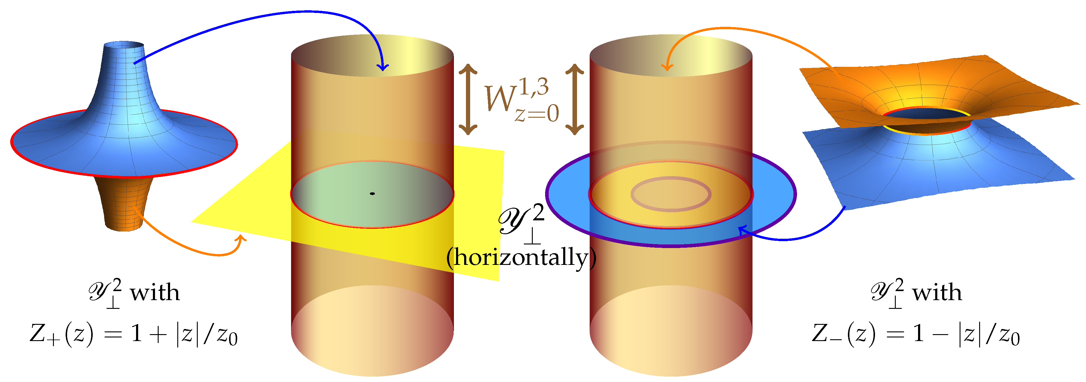
| 6 | To be precise: for in (4a), each of the two circular boundaries of shrinks to a point as , thus rendering compact. For in (4a), is non-compact and two points must be added to compactify . |
| 7 | We will return to this non-trivial K3-fibration in Section 4. |
| 8 | The product denotes that the warp-factors in the block-diagonal metric vary over . |
| 9 | Being Fano, , implies the scalar curvature invariant to be positive, . |
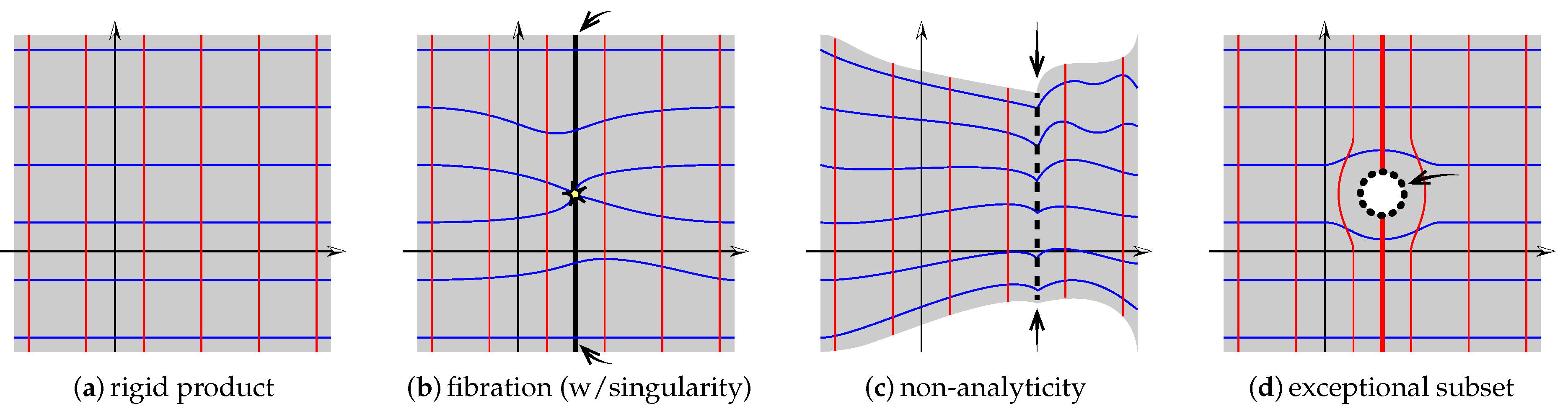
| 10 | For our present purposes, a foliation means that the total space looks locally at every point as a direct product of local portions of the two factors, X and Y. |
| 11 | Supersymmetry is in string theory largely correlated with complex structure, and as mentioned above, of course admits a complex structure, for which the excised point is an obstruction. |
| 12 | This may be pictured as a two-step process: (1) “open” the point into a circular boundary, then (2) identify segments of the boundary according to the template in Figure A1, middle. |
References
- Riess, A.G.; Filippenko, A.V.; Challis, P.; Clocchiatti, A.; Diercks, A.; Garnavich, P.M.; Gilliland, R.L.; Hogan, C.J.; Jha, S.; Kirshner, R.P.; et al. Observational evidence from supernovae for an accelerating universe and a cosmological constant. Astron. J. 1998, 116, 1009–1038. [Google Scholar] [CrossRef]
- Perlmutter, S.; Aldering, G.; Goldhaber, G.; Knop, R.A.; Nugent, P.; Castro, P.G.; Deustua, S.; Fabbro, S.; Goobar, A.; Groom, D.E.; et al. Measurements of Omega and Lambda from 42 high redshift supernovae. Astrophys. J. 1999, 517, 565–586. [Google Scholar] [CrossRef]
- Danielsson, U.H.; Van Riet, T. What if string theory has no de Sitter vacua? Int. J. Mod. Phys. 2018, D27, 1830007. [Google Scholar] [CrossRef]
- Cicoli, M.; De Alwis, S.; Maharana, A.; Muia, F.; Quevedo, F. De Sitter vs Quintessence in String Theory. Fortsch. Phys. 2018, 2018, 1800079. [Google Scholar] [CrossRef]
- Berglund, P.; Hübsch, T.; Minic, D. On de Sitter Spacetime and String Theory, to appear.
- Banerjee, S.; Danielsson, U.; Dibitetto, G.; Giri, S.; Schillo, M. Emergent de Sitter Cosmology from Decaying Anti–de Sitter Space. Phys. Rev. Lett. 2018, 121, 261301. [Google Scholar] [CrossRef]
- Banerjee, S.; Danielsson, U.; Dibitetto, G.; Giri, S.; Schillo, M. De Sitter Cosmology on an expanding bubble. J. High Energy Phys. 2019, 10, 164. [Google Scholar] [CrossRef]
- Bento, B.V.; Chakraborty, D.; Parameswaran, S.L.; Zavala, I. A New de Sitter Solution with a Weakly Warped Deformed Conifold. arXiv 2021, arXiv:2105.03370. [Google Scholar]
- Blåbäck, J.; Danielsson, U.; Dibitetto, G.; Giri, S. Constructing stable de Sitter in M-theory from higher curvature corrections. J. High Energy Phys. 2019, 2019, 1–24. [Google Scholar] [CrossRef]
- Berglund, P.; Hübsch, T.; Minic, D. Exponential Hierarchy From Spacetime Variable String Vacua. J. High Energy Phys. 2000, 9, 15. [Google Scholar] [CrossRef][Green Version]
- Berglund, P.; Hübsch, T.; Minic, D. Probing Naked Singularities in Non-supersymmetric String Vacua. J. High Energy Phys. 2001, 2, 10. [Google Scholar] [CrossRef][Green Version]
- Berglund, P.; Hübsch, T.; Minic, D. Localized Gravity and Large Hierarchy from String Theory? Phys. Lett. 2001, 512, 155–160. [Google Scholar] [CrossRef][Green Version]
- Berglund, P.; Hübsch, T.; Minic, D. De Sitter Spacetimes from Warped Compactifications of IIB String Theory. Phys. Lett. 2002, 534, 147–154. [Google Scholar] [CrossRef]
- Berglund, P.; Hübsch, T.; Minic, D. On Stringy de Sitter Spacetimes. J. High Energy Phys. 2019, 2019, 166. [Google Scholar] [CrossRef]
- Berglund, P.; Hübsch, T.; Minic, D. String Theory, the Dark Sector and the Hierarchy Problem. LHEP 2021, 2021, 186. [Google Scholar] [CrossRef]
- Hübsch, T. A Hitchhiker’s Guide to Superstring Jump Gates and Other Worlds. Nucl. Phys. Proc. Suppl. 1997, 52A, 347–351. [Google Scholar] [CrossRef]
- Dixon, L.J.; Harvey, J.A.; Vafa, C.; Witten, E. Strings on Orbifolds. Nucl. Phys. B 1985, 261, 678–686. [Google Scholar] [CrossRef]
- Dixon, L.J.; Harvey, J.A.; Vafa, C.; Witten, E. Strings on Orbifolds. 2. Nucl. Phys. B 1986, 274, 285–314. [Google Scholar] [CrossRef]
- Green, P.S.; Hübsch, T. Connecting Moduli Spaces of Calabi-Yau Threefolds. Commun. Math. Phys. 1988, 119, 431–441. [Google Scholar] [CrossRef]
- Green, P.S.; Hübsch, T. Possible Phase Transitions Among Calabi-Yau Compactifications. Phys. Rev. Lett. 1988, 61, 1163–1166. [Google Scholar] [CrossRef]
- Candelas, P.; Green, P.S.; Hübsch, T. Rolling Among Calabi-Yau Vacua. Nucl. Phys. B 1990, 330, 49–102. [Google Scholar] [CrossRef]
- Partouche, H.; Pioline, B. Rolling among G(2) vacua. J. High Energy Phys. 2001, 3, 5. [Google Scholar] [CrossRef]
- Aspinwall, P.S.; Greene, B.R.; Morrison, D.R. Calabi–Yau moduli space, mirror manifolds and space-time topology change in string theory. Nucl. Phys. B 1994, 416, 414–480. [Google Scholar] [CrossRef]
- Aspinwall, P.S.; Greene, B.R.; Morrison, D.R. Space-time topology change and stringy geometry. J. Math. Phys. 1994, 35, 5321–5337. [Google Scholar] [CrossRef]
- Strominger, A. Massless black holes and conifolds in string theory. Nucl. Phys. B 1995, 451, 96–108. [Google Scholar] [CrossRef]
- Hubsch, T.; Rahman, A. On the geometry and homology of certain simple stratified varieties. J. Geom. Phys. 2005, 53, 31–48. [Google Scholar] [CrossRef]
- Polchinski, J.; Chaudhuri, S.; Johnson, C.V. Notes on D-branes. arXiv 1996, arXiv:hep-th/9602052. [Google Scholar]
- Sagnotti, A. Open Strings and Their Symmetry Groups; NATO Advanced Summer Institute on Nonperturbative Quantum Field Theory (Cargese Summer Institute); Plenum Press: New York, NY, USA, 1987. [Google Scholar]
- Horava, P. Strings on World Sheet Orbifolds. Nucl. Phys. B 1989, 327, 461–484. [Google Scholar] [CrossRef]
- Bianchi, M.; Sagnotti, A. Twist symmetry and open string Wilson lines. Nucl. Phys. B 1991, 361, 519–538. [Google Scholar] [CrossRef]
- Klebanov, I.R.; Strassler, M.J. Supergravity and a confining gauge theory: Duality cascades and chi SB resolution of naked singularities. J. High Energy Phys. 2000, 8, 52. [Google Scholar] [CrossRef]
- DeWolfe, O.; Giddings, S.B. Scales and hierarchies in warped compactifications and brane worlds. Phys. Rev. D 2003, 67, 066008. [Google Scholar] [CrossRef]
- Douglas, M.R.; Shelton, J.; Torroba, G. Warping and supersymmetry breaking. arXiv 2007, arXiv:0704.4001. [Google Scholar]
- Douglas, M.R. Effective potential and warp factor dynamics. J. High Energy Phys. 2010, 3, 71. [Google Scholar] [CrossRef]
- Bena, I.; Graña, M.; Halmagyi, N. On the Existence of Meta-stable Vacua in Klebanov-Strassler. J. High Energy Phys. 2010, 9, 87. [Google Scholar] [CrossRef]
- Bena, I.; Graña, M. String cosmology and the landscape. Comptes Rendus Phys. 2017, 18, 200–206. [Google Scholar] [CrossRef]
- Eguchi, T.; Hanson, A.J. Selfdual Solutions to Euclidean Gravity. Ann. Phys. 1979, 120, 82. [Google Scholar] [CrossRef]
- Gibbons, G.W.; Pope, C.N. CP2 as a gravitational Instanton. Commun. Math. Phys. 1978, 61, 239–248. [Google Scholar] [CrossRef]
- Hübsch, T. Calabi-Yau Manifolds: A Bestiary for Physicists, 2nd ed.; World Scientific Publishing Co. Inc.: River Edge, NJ, USA, 1994. [Google Scholar]
- Hartshorne, R. Algebraic Geometry; Springer: New York, NY, USA, 1977. [Google Scholar]
- Reid, M. The moduli space of 3-folds with K=0 may nevertheless be irreducible. Math. Ann. 1987, 278, 329–334. [Google Scholar] [CrossRef]
- Greene, B.R.; Shapere, A.D.; Vafa, C.; Yau, S.T. Stringy Cosmic Strings and Noncompact Calabi–Yau Manifolds. Nucl. Phys. B 1990, 337, 1–36. [Google Scholar] [CrossRef]
- Green, P.S.; Hübsch, T. Spacetime Variable String Vacua. Int. J. Mod. Phys. A 1994, 9, 3203–3228. [Google Scholar] [CrossRef]
- Randall, L.; Sundrum, R. A Large mass hierarchy from a small extra dimension. Phys. Rev. Lett. 1999, 83, 3370–3373. [Google Scholar] [CrossRef]
- Randall, L.; Sundrum, R. An Alternative to compactification. Phys. Rev. Lett. 1999, 83, 4690–4693. [Google Scholar] [CrossRef]
- Hawking, S.W.; Hertog, T.; Reall, H.S. Brane new world. Phys. Rev. D 2000, 62, 043501. [Google Scholar] [CrossRef]
- Karch, A.; Randall, L. Locally localized gravity. J. High Energy Phys. 2001, 2001, 8. [Google Scholar] [CrossRef]
- Danielsson, U.H.; Panizo, D.; Tielemans, R.; Riet, T.V. A higher-dimensional view on quantum cosmology. arXiv 2021, arXiv:2105.03253. [Google Scholar]
- Basile, I.; Lanza, S. De Sitter in non-supersymmetric string theories: No-go theorems and brane-worlds. J. High Energy Phys. 2020, 10, 108. [Google Scholar] [CrossRef]
- Coleman, S.R.; De Luccia, F. Gravitational Effects on and of Vacuum Decay. Phys. Rev. D 1980, 21, 3305. [Google Scholar] [CrossRef]
- Banks, T.; Zhang, B. Comment on Coleman-DeLuccia Instantons. arXiv 2021, arXiv:2106.12696. [Google Scholar]
- Ooguri, H.; Vafa, C. Non-supersymmetric AdS and the Swampland. Adv. Theor. Math. Phys. 2017, 21, 1787–1801. [Google Scholar] [CrossRef]
- Freivogel, B.; Kleban, M. Vacua Morghulis. arXiv 2016, arXiv:1610.04564. [Google Scholar]
- Danielsson, U.H.; Dibitetto, G.; Vargas, S.C. Universal isolation in the AdS landscape. Phys. Rev. D 2016, 94, 126002. [Google Scholar] [CrossRef]
- McNamara, J.; Vafa, C. Cobordism Classes and the Swampland. arXiv 2019, arXiv:1909.10355. [Google Scholar]
- Polchinski, J. String Theory. Vol. 1: An Introduction to the Bosonic String; Cambridge Monographs on Mathematical Physics; Cambridge University Press: Cambridge, UK, 2007. [Google Scholar]
- Friedan, D.H. Nonlinear Models in 2+ϵ Dimensions. Phys. Rev. Lett. 1980, 45, 1057. [Google Scholar] [CrossRef]
- Friedan, D.H. Nonlinear Models in 2+ϵ Dimensions. Ann. Phys. 1985, 163, 318–419. [Google Scholar] [CrossRef]
- Shapere, A.D.; Wilczek, F. (Eds.) Geometric Phases in Physics; Advanced Series in Mathematical Physics, World Sci. Publishing: Singapore, 1989; Volume 5. [Google Scholar]
- Hull, C.; Israel, D.; Sarti, A. Non-geometric Calabi-Yau Backgrounds and K3 automorphisms. J. High Energy Phys. 2017, 11, 84. [Google Scholar] [CrossRef]
- Nemeschansky, D.; Sen, A. Conformal Invariance of Supersymmetric σ Models on Calabi-yau Manifolds. Phys. Lett. B 1986, 178, 365–369. [Google Scholar] [CrossRef]
- Douglas, M.R.; Kachru, S. Flux compactification. Rev. Mod. Phys. 2007, 79, 733–796. [Google Scholar] [CrossRef]
- Grana, M. Flux compactifications in string theory: A Comprehensive review. Phys. Rep. 2006, 423, 91–158. [Google Scholar] [CrossRef]
- Frenkel, I.B.; Garland, H.; Zuckerman, G.J. Semiinfinite Cohomology and String Theory. Proc. Nat. Acad. Sci. USA 1986, 83, 8442. [Google Scholar] [CrossRef]
- Bowick, M.J.; Yang, K.Q. String Equations of Motion from Vanishing Curvature. Int. J. Mod. Phys. 1991, A6, 1319–1334. [Google Scholar] [CrossRef]
- Bowick, M.J.; Lahiri, A. The Ricci Curvature of Diff S1/ SL(2,R). J. Math. Phys. 1988, 29, 1979. [Google Scholar] [CrossRef]
- Bowick, M.J.; Rajeev, S. The Complex Geometry of String Theory and Loop Space. In Johns Hopkins Workshop on Current Problems in Particle Theory; Duan, Y.S., Domókos, G., Kövesi-Domókos, S., Eds.; World Sci. Publishing: Singapore, 1987. [Google Scholar]
- Bowick, M.J.; Rajeev, S.G. Anomalies and Curvature in Complex Geometry. Nucl. Phys. B 1988, 296, 1007–1033. [Google Scholar] [CrossRef]
- Bowick, M.J.; Rajeev, S.G. The Holomorphic Geometry of Closed Bosonic String Theory and DiffS1/S1. Nucl. Phys. B 1987, 293, 348. [Google Scholar] [CrossRef]
- Bowick, M.J.; Rajeev, S.G. String Theory as the Kahler Geometry of Loop Space. Phys. Rev. Lett. 1987, 58, 535. [Google Scholar] [CrossRef]
- Alvarez-Gaume, L.; Gomez, C.; Reina, C. Loop groups, Grassmanians and string theory. Phys. Lett. B 1987, 190, 55. [Google Scholar] [CrossRef]
- Oh, P.; Ramond, P. Curvature of Superdiff S1/S1. Phys. Lett. B 1987, 195, 130–134. [Google Scholar] [CrossRef]
- Harari, D.; Hong, D.K.; Ramond, P.; Rodgers, V.G.J. The Superstring DiffS1/S1 and Holomorphic Geometry. Nucl. Phys. B 1987, 294, 556–572. [Google Scholar] [CrossRef]
- Pilch, K.; Warner, N.P. Holomorphic Structure of Superstring Vacua. Class. Quant. Grav. 1987, 4, 1183. [Google Scholar] [CrossRef]
- Freidel, L.; Leigh, R.G.; Minic, D. Metastring Theory and Modular Space-time. J. High Energy Phys. 2015, 2015, 1–76. [Google Scholar] [CrossRef]
- Freidel, L.; Leigh, R.G.; Minic, D. Intrinsic non-commutativity of closed string theory. J. High Energy Phys. 2017, 2017, 1–24. [Google Scholar] [CrossRef]
- Freidel, L.; Leigh, R.G.; Minic, D. Noncommutativity of closed string zero modes. Phys. Rev. D 2017, 96, 066003. [Google Scholar] [CrossRef]
- Tian, G.; Yau, S.T. Complete Kähler manifolds with zero Ricci curvature. I. J. Am. Math. Soc. 1990, 3, 579–609. [Google Scholar]
- Tian, G.; Yau, S.T. Complete Kähler manifolds with zero Ricci curvature. II. Invent. Math. 1991, 106, 27–60. [Google Scholar] [CrossRef]
- Witten, E. Instability of the Kaluza-Klein Vacuum. Nucl. Phys. B 1982, 195, 481–492. [Google Scholar] [CrossRef]
- Dibitetto, G.; Petri, N.; Schillo, M. Nothing really matters. J. High Energy Phys. 2020, 2020, 1–19. [Google Scholar] [CrossRef]
- Green, P.S.; Hübsch, T. Calabi-Yau Hypersurfaces in Products of Semi-Ample Surfaces. Commun. Math. Phys. 1988, 115, 231–246. [Google Scholar] [CrossRef]


Publisher’s Note: MDPI stays neutral with regard to jurisdictional claims in published maps and institutional affiliations. |
© 2021 by the authors. Licensee MDPI, Basel, Switzerland. This article is an open access article distributed under the terms and conditions of the Creative Commons Attribution (CC BY) license (https://creativecommons.org/licenses/by/4.0/).
Share and Cite
Berglund, P.; Hübsch, T.; Minic, D. Stringy Bubbles Solve de Sitter Troubles. Universe 2021, 7, 363. https://doi.org/10.3390/universe7100363
Berglund P, Hübsch T, Minic D. Stringy Bubbles Solve de Sitter Troubles. Universe. 2021; 7(10):363. https://doi.org/10.3390/universe7100363
Chicago/Turabian StyleBerglund, Per, Tristan Hübsch, and Djordje Minic. 2021. "Stringy Bubbles Solve de Sitter Troubles" Universe 7, no. 10: 363. https://doi.org/10.3390/universe7100363
APA StyleBerglund, P., Hübsch, T., & Minic, D. (2021). Stringy Bubbles Solve de Sitter Troubles. Universe, 7(10), 363. https://doi.org/10.3390/universe7100363