Abstract
Ever since Eddington’s analysis of the gravitational redshift a century ago, and the arguments in the relativity community that it produced, fine details of the roles of proper time and coordinate time in the redshift remain somewhat obscure. We shed light on these roles by appealing to the physics of the uniformly accelerated frame, in which coordinate time and proper time are well defined and easy to understand; and because that frame exists in flat spacetime, special relativity is sufficient to analyse it. We conclude that Eddington’s analysis was indeed correct—as was the 1980 analysis of his detractors, Earman and Glymour, who (it turns out) were following a different route. We also use the uniformly accelerated frame to pronounce invalid Schild’s old argument for spacetime curvature, which has been reproduced by many authors as a pedagogical introduction to curved spacetime. More generally, because the uniformly accelerated frame simulates a gravitational field, it can play a strong role in discussions of proper and coordinate times in advanced relativity.
1. Introduction
The prediction and subsequent confirmation of gravitational redshift is a standard topic of courses on general relativity. Despite this, the meanings and roles of the two times used in the analysis have produced differences of opinion historically. In [1], Scott describes how Eddington [2,3] derived the standard result by analysing the relationship of proper and coordinate times at two heights in a gravitational field. Eddington’s analysis used the language of his day, and while it gives the correct result, its logic was questioned even in Eddington’s time. This calculation was essentially reproduced by later authors, such as Weinberg [4]. The analysis was critiqued by Earman and Glymour [5], who swapped the roles of proper and coordinate time in what appeared to be a very similar calculation, and yet produced the same, correct, expression for the redshift that Eddington derived. The natural question arises: what are the correct roles of proper and coordinate times in the gravitational redshift, and why did these apparently contrasting analyses both yield the correct result?
The purpose of this paper is to show how the roles and correct use of proper and coordinate times arise naturally in a flat spacetime context, when we analyse the pseudo-gravitational redshift that appears in the uniformly accelerated frame in flat spacetime (UAF). Because the UAF mimics a gravitational field over small differences in “height”, the equivalence principle guarantees that it forms a good test-bed for discussing the redshift in curved spacetime.1 Despite this utility, the UAF is almost absent from textbooks on relativity; even Misner, Thorne and Wheeler’s comprehensive textbook [6] devotes only a few pages to it. In-depth discussions of the UAF can certainly be found in studies of the foundational aspects of relativity, such as in [7,8,9,10,11,12]. But study of the UAF is perhaps still regarded as the province of a small group of specialists. I believe that a good understanding of the roles of proper and coordinate times in the UAF can be obtained by following the specifics of how the frame and its coordinates are constructed. Those details appear in Section 4.
Discussions of relativity demand a careful use of jargon. Throughout this paper, we distinguish “seeing” from “observing”. Seeing is what we do with our eyes, and is subject to any “tricks of the light” that might arise in a scenario. In contrast, “observing” or “measuring” describes what is really happening, and is what results after allowance has been made for the time taken by a signal from an event to reach an observer. In this paper, we will use two observers, Alice and Bob; but it’s important to realise that each observation belongs to the frame as a whole, independently of who made the actual measurement. All observers in the frame agree on any given observation, and the “person observing the event” has merely constructed the observation from all the information available. In analyses, it is equivalent but simpler to treat spacetime as populated by a continuum of observers who each record events only in their own immediate neighbourhood. These records are then passed to a master observer, who collates the information and builds a description of what happened when and where. This description becomes the observation or measurement of a scenario.
For example, when we stand on a platform in an inertial frame and watch a train go by, the Doppler effect ensures that we see the clocks of approaching passengers ticking faster than those of receding passengers; but when this purely visual position-dependent effect is subtracted from the data, we—and all the other observers in our platform frame—observe or measure all the train’s clocks to tick at the same rate, slower than our own by the usual gamma factor. In fact, we will find that in our redshift scenario, seeing turns out to be the same as observing; but that fact must be acknowledged explicitly in any analysis. What everyone sees is interesting in its own right, but it must be distinguished from what everyone observes.
The rate of ticking of a clock (a pseudonym for all physical processes) might be quantified in two ways. Its coordinate rate is the number of ticks per unit coordinate time. This rate can vary, and is referred to when an inertial observer says “A moving clock ticks slowly”. A clock’s proper rate is the number of ticks per unit proper time; since the tick defines the proper time, this proper rate never varies, and is somewhat trivial to speak of. In the famous twin paradox of Section 4.5, when one says that space-bound Bob ages more slowly than Earthbound Alice, it is the coordinate tick rate of Bob’s ageing process that is lower than that of Alice. This difference is tangible, and Bob is younger than Alice on his return to Earth. Throughout this paper, when we refer to clocks’ rates varying, we always mean their coordinate rates, in agreement with normal relativity usage. But being aware of coordinate and proper rates is a useful step for the idea of coordinate frequency versus proper frequency in Section 9.
2. Eddington’s Prediction of Gravitational Redshift
We present here a rewording of Scott’s description of Eddington’s prediction of the redshift undergone by light climbing up a real gravitational field. We replace Scott’s infinitesimal “d” with a non-infinitesimal “”, and momentarily postpone questions of what the analysis is really doing.
Observers Alice and Bob are at rest in a static gravitational field, with Alice at a lower potential than Bob. She sends Bob a light signal that climbs up the potential. Our task is to determine whether and by how much Bob observes a different frequency in the received signal, and whether he sees anything different from what he observes. Energy conservation and the quantum-mechanical postulate “energy ∝ frequency” (discussed in Section 9) suggest that Bob should see a redshift. In this case, because Bob and Alice have no relative motion, “seeing” is the same as “observing/measuring”, since no kinematic Doppler shift is present.
Eddington gives Alice and Bob identical clocks whose “proper period” of oscillation is some . That is, if this period is one second, then Alice and Bob can each say “During one period of my clock, I grew older by one second”. The metric relates this period to the frame’s coordinate time t by , where is the time component of the metric. Eddington says (and note that we have changed his sometimes-obscure wording) that Alice measures her clock to have a “coordinate period” , meaning the coordinate time at Alice’s location that elapses between successive ticks. Bob measures his clock likewise to have a coordinate period . Eddington thus effectively writes (where throughout this paper, A stands for Alice and B for Bob)
Denote by the frequency measured by Alice of her clock, and similarly for Bob and his clock. Eddington then has
It can be shown [13] from an analysis of geodesic motion in a weak static gravitational potential (chosen to tend to zero at “infinite height”) that . It follows that . We then infer from (2) that , and indeed that, in weak gravity,
Eddington concludes that Bob measures his clock’s tick rate to be higher than the value that Alice measures for her clock’s tick rate, and hence that Bob sees light emitted by Alice as redshifted by the difference in potentials. Eddington’s result has been verified experimentally, and (3) is now established as the correct expression for the redshift.
The above is a paraphrase of Eddington’s analysis in modern language, but his own description in [3] was far more cursory. We can ask if redshift is even present in his discussion of tick rates. Seeing and observing are the same in this scenario, and that means what Bob sees is what is really taking place; so, since he sees Alice’s clocks ticking slowly (and hence Alice ageing slowly), he must also see a lower frequency of the light she produces. It’s not clear if this fact was recognised or given much attention in Eddington’s time. Eddington’s abbreviated reasoning was questioned in his own day, as discussed in detail in [1,5]. Those questions were from an era when ideas of proper time and coordinate time were new, and we will return to them later.
Eddington’s derivation and variations on it have been reproduced by other physicists, as discussed by Earman and Glymour in [5]. Earman and Glymour gave their own derivation of the redshift that centres around their Equations (2.4) to (2.5″) in [5]. In our language of Alice and Bob, they define
Additionally, for any light that Bob might emit, they define
although this just equals because Alice and Bob’s clocks were manufactured identically. They then state, in essence, that for some ,
Hence,
That is, Bob measures a lower frequency of Alice’s light than Alice measures—hence, a redshift. Earman and Glymour were attempting to fix Eddington’s derivation, which they described as “exactly backwards from what is wanted”, owing to what they called Eddington’s “misapplication” of ideas. Likewise, they pronounced incorrect Einstein’s derivation, which was essentially the same as Eddington’s. We’ll see in this paper that although Earman–Glymour’s re-derivation was as correct (and as obscure) as Eddington’s, they misunderstood what he was doing.
In general discussions, special relativity teaches us to isolate, say, events 1 and 2 of interest. In a frame called S, we write , and in we refer to the same two events by writing . The Lorentz transform then connects to , and everything is well defined. But in the arguments above, the meanings of the time increments are not necessarily clear. Do they refer to ticks of a clock or crests of a wave? What specific events are being observed?
We will construct a UAF formalism that allows a clear analysis of both redshift derivations. We’ll see in Section 8 that the approaches of both Eddington and Earman–Glymour were correct; they were simply doing different things. The derivation of Eddington (and Einstein) was not “backwards” at all. Eddington examined the lapses in coordinate time for two equal proper times; Earman–Glymour examined the lapses in proper time for two equal coordinate times.
Gravitational redshift is often predicted or interpreted using a completely different approach to that of Eddington. That other approach calculates a drop in frequency of Alice’s emitted ray en route to Bob, in accordance with energy conservation in a weak non-relativistic gravitational field. In [14], Okun et al. maintain that the energy-conservation approach is incorrect. In Section 9, we’ll discuss Okun’s view in a UAF context.
3. Acceleration and the Flow of Time
The accelerated frame is rarely analysed in any detail in introductory textbooks in special relativity, but its core feature is already evident in those books. As taught in all introductory courses, when a train with two on-board identical clocks synchronised and at rest on the train moves with constant velocity v through our inertial frame, we say that although the clocks tick at identical rates in our frame, the rear clock displays ahead of the front clock by a time , where their proper separation is . We also learn that time’s “rate of flow” is defined by the ticking (ageing, if you prefer) of an ideal clock. In this paper, we’ll discuss “gearing” clocks to tick at different speeds, and will then distinguish an arbitrarily manufactured tick rate from the clock’s immutable ageing rate. It is then the ageing rate that defines the flow of time.
Now, suppose that one of two synchronised clocks sits by our side, while the other lies in a distant galaxy, one thousand million light-years away. Leaving aside questions of cosmological distance, their proper separation is light-years. Suppose that we on Earth pace slowly back and forth, moving with speed in each direction. In that case, the clock next to us alternately leads and trails its partner by one year. But because it is right next to us, we can see and observe that its time is not changing at all by any more than the few seconds we spend pacing. This implies that the clock in the distant galaxy is alternately jumping ahead of us by one year and then suddenly dropping behind by the same amount; and this see-sawing continues for as long as we pace back and forth. We conclude that the display on the distant clock really is swinging back and forth—implying time in that galaxy is behaving likewise—as we accelerate periodically to switch our walking direction.2 Already in this simple scenario, the rates of clocks in an accelerated frame are position dependent. Hence, a position-dependent rate of flow of time must emerge from any analysis of an accelerated frame.
This position-dependent rate of flow of time in an accelerated frame implies that the speed of light in that frame is also position dependent. (To see this, consider running a movie at high speed: everything in that movie moves faster, including a light beam that sets events into motion.) This rules out at least any simplistic use of radar to measure or define distances in an accelerated frame. Radar requires knowing the speed of light at all points between emitter and receiver; but, since this can vary with position, one cannot simply invoke “distance signal-travel time” globally. (Cook [15] defines a “local [infinitesimal] radar distance” using c, in the context of a frame, where each infinitesimal distance applies to one of a chain of observers, each applying “distance signal-travel time” in their immediate vicinity. But in general, a frame cannot be constructed by a chain of observers with arbitrarily differing motions. If it could, we would be permitted to chain together the differently moving inertial observers/frames in an introductory relativity textbook, , etc., to build a “frame” that disobeyed the basic rules of special relativity.) In addition, using radar to synchronise clocks in an accelerated frame presupposes that those clocks age at the same rate, but the above discussion of pacing back and forth shows that they do not age at the same rate.
4. Constructing the UAF
The UAF springs from this question: is it possible for a frame to exist in flat spacetime whose observers each feel a fixed acceleration for all time? To answer this, we must define a frame carefully. As described in [16], we take a frame to be a collection of observers who require that:
- Any two events deemed simultaneous by one observer are deemed simultaneous by all observers. This requirement enables them to construct a time coordinate that serves the whole frame. This coordinate time is normally chosen to be the proper time—the “age”—of one of the observers (the “master observer”), and need not match the proper times (the ages) of other observers. If all observers are given identical clocks, then the observers who age faster (slower) than the master observer gear their clocks down (up), making them all agree that all clocks display any given time simultaneously. We must now distinguish an observer/clock’s ageing rate from a clock’s tick rate. Picture an ageing rate as biological, set by the laws of physics and unable to be changed by us; and a tick rate as mechanical and arbitrary, set by gear wheels that we can prepare in any way we choose;
- All separations between the observers are deemed by them to be constant. The observers thus form a rigid lattice, allowing them to construct a single set of space coordinates that serve the whole frame.
This definition of a frame and its coordinates (at least applying to flat spacetime) is stringent. Compare it with the definition given in [7,17], which is simply that a frame is a collection of observers with non-crossing world lines, with no stipulation of any notion of “frame-wide” simultaneity. In contrast, our definition above requires frame-wide simultaneity. For an example of a time coordinate that is not related to simultaneity, look no further than a textbook introduction to special relativity: the time coordinates that conventionally describe two inertial frames certainly each define frame-wide simultaneity for its relevant frame; but, because the Lorentz transformation converts between unprimed and primed coordinates unambiguously, nothing stops us from using t as a coordinate in . Although a valid coordinate, t does not match the frame-wide simultaneity in , and hence does not fit with the first requirement above.
Discussions of the UAF (including ours) probably universally define simultaneity for any UAF observer at each moment to match that of his momentarily comoving inertial frame (MCIF) at that moment. The MCIF is an inertial frame that, at the moment in which it applies, shares the same velocity as the observer.3 Simultaneity in inertial frames is well understood. Defining simultaneity in the UAF using MCIFs is useful and meaningful because it predicts a redshift in the UAF which, when applied to real gravity using the equivalence principle, is confirmed by experiment.
An observer cannot hold a fixed acceleration forever in the “laboratory inertial frame”, as measured by that frame. (We will always take the lab to be inertial.) But because a constant velocity cannot be felt, the acceleration felt by the observer at any given moment is his velocity change relative to his current MCIF, not relative to the lab. The world line of a linearly accelerated observer who feels a constant acceleration to the right turns out to be a hyperbola that asymptotes from the leftward lab speed of light in the distant past to the rightward lab speed of light in the distant future [7,18].
Use of the MCIF is closely allied to the clock postulate of special relativity. Consider an observer riding in an accelerating train on a straight track next to another train that holds a fixed velocity. At some moment, the accelerating train’s velocity will equal that of the inertial train. When that happens, for a brief time, it’s reasonable that any passenger on the accelerating train should be able to lean out of the window and converse with the nearest passenger on the inertial train: they should each even be able to run identical physics experiments and agree on the results. For the short duration of their conversing, the inertial train is the MCIF of the accelerating observer. The clock postulate states that the observations an accelerating observer makes of events in his vicinity should always match those of his current MCIF. In particular, each observer, accelerated and inertial, should note that the other’s clock ticks at the same rate as his own.
The clock postulate says that the tick rate of a clock that accelerates in the inertial lab slows by the usual -factor of special relativity, which is now a function of time: ; here, is the speed of the accelerated clock in the lab. That is, contains no time derivatives of . The clock postulate has been tested under extreme accelerations, as high as times Earth’s gravity [19,20]. The postulate also applies to the shortening of rods, and to energy/momentum, since these are measurements set by the MCIF’s -factor. And it applies in the presence of real gravity.
4.1. A Lattice of Observers for the UAF
Building the UAF begins with the above observation that the world line of an observer who feels a fixed acceleration g in the inertial (gravity-free) lab frame S is a hyperbola. With suitable initial conditions, his world line in lab coordinates is (with ) [6,18]
where “sh, ch” are the hyperbolic functions sinh and cosh (and later, “th” for tanh), and is the observer’s proper time: his biological age. (We will allow this age to be negative.)
Equation (8) describes us firing our rocket motors to accelerate forever, as shown in Figure 1. We start out far in the past and move left toward , always firing our rocket to produce what we feel as a fixed acceleration g in the positive-x direction. Eventually we slow to a stop at and , reverse direction, and pick up speed again, now moving to the right, away from the origin. In conventional units, becomes , and for one Earth gravity, is very close to one light-year.
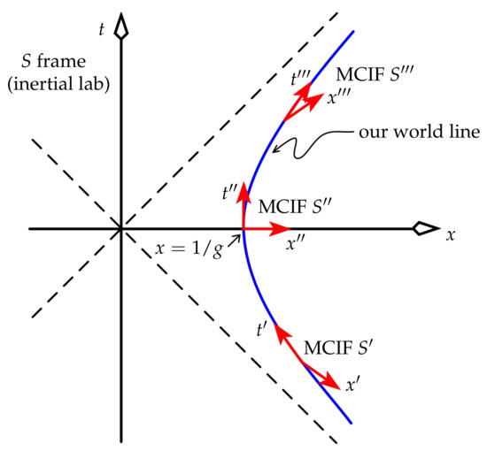
Figure 1.
Our hyperbolic world line in the inertial frame S of the lab. Included are a selection of the infinite number of our MCIFs. The positive-x direction is “up” for us, in the sense that we feel a force pressing us into our seats “downward” in the negative-x direction.
Figure 1 includes a selection of MCIFs, represented by their spacetime axes. The time axis of each MCIF has slope , where v is the (constant) velocity of that MCIF in S. The space axis has slope v: it is orthogonal in the Minkowski sense to the time axis.
To ascertain if we can construct a global frame based on our motion, we must address point 1 at the start of Section 4. Draw the line of simultaneity through an arbitrary event on our hyperbolic world line by noting that the tangent there has slope , and so the corresponding line of simultaneity has slope . Equation (8) says that . Hence, the line of simultaneity at event has slope , and so it passes through the origin of S, . This spacetime-origin event, then, is simultaneous with every event on our world line, past and future. This and other strange phenomena result from the extremely non-physical nature of our world line. To say that we have been, and are, accelerating forever in a flat spacetime is a very strong statement about the entire universe, and about time in general.
If we now place other observers in the lab with appropriate hyperbolic world lines, they will also draw their lines of simultaneity through . Hence, they will all agree with us on simultaneity. Three of these observers’ world lines are drawn in Figure 2. In the same way that our world line satisfies (8), bringing us to rest at where g is our acceleration, another accelerating observer i has a constant acceleration in S, with a turn-around point of . All such observers agree with us on which events are happening “now”. Also, along each common line of simultaneity, all observers’ four-velocities are parallel, since these four-velocities are all orthogonal to that line of simultaneity. It follows that, in each observer’s MCIF, the world lines of all other observers maintain a constant separation. Thus, they measure each other always to be at rest with respect to themselves, and hence they say that they form a rigid lattice of observers who all agree on simultaneity. Hence, by points 1 and 2 in Section 4, they form a frame. This is the UAF, which we call throughout this paper. Note that the UAF covers only one quarter of spacetime, shaded yellow in Figure 2 and often called Rindler spacetime. Despite being flat, it has much in common with Schwarzschild spacetime, as evidenced by the mathematical similarity of Figure 2 with the Kruskal–Szekeres coordinates that are usually invoked to analyse Schwarzschild spacetime [21]. In [17], Desloge argues that the UAF is the only well-defined frame obeying the requirements at the start of Section 4, other than the inertial frame.4
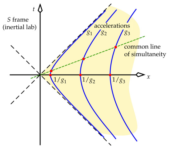
Figure 2.
Three of the continuum of observers who help us make measurements. When their accelerations in their MCIFs bring them momentarily to rest at positions given by those accelerations’ reciprocals (really , etc., in conventional distance units), then the geometry of hyperbolae guarantees that these observers will always share a common line of simultaneity, as required to make a well-defined frame. This frame covers only the quarter of spacetime shaded yellow. The bunching up of the observers in the future and past (times when they move quickly) is the Lorentz contraction.
Because observers at varying “heights” x in the UAF feel different accelerations, the standard word “uniform” in “uniformly accelerated frame” is something of a misnomer, and certainly doesn’t imply equal accelerations for all observers. The UAF’s observers have differing accelerations in the lab, and hence don’t form a rigid lattice there; but they say that they do form a rigid lattice. Conversely, if a set of observers are each given the same acceleration in the lab, then they say they are moving relative to each other and do not form a rigid lattice.
The UAF gives insight into “Bell’s rocket paradox”. When two observers accelerate in the same direction, the chasing observer must accelerate more strongly than the leading observer if the observers are to measure the distance between them as remaining constant. These observers follow the world lines in Figure 2. (The bunching up of the observers in the future and past in Figure 2 is precisely the Lorentz contraction.) On the other hand, if the observers accelerate identically, the chasing observer does not accelerate fast enough to create the UAF, and so the observers measure their separation to increase. Any string that joins them—without being accelerated independently of the observers—must then break. John Bell famously put the following question to his fellow physicists: “If two rockets accelerate identically in the same direction, what will happen to a string joining them?”. Two such rockets will measure their separation to be increasing, and so a string connecting them must snap.
4.2. Coordinates for the UAF
We now coordinatise the UAF. The clocks of must be calibrated to all agree that they display the same value, , at each moment; this becomes the coordinate time of . Refer to Figure 3, which shows two UAF observers, Alice and Bob.
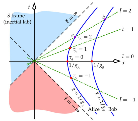
Figure 3.
An event’s value of is defined to be the proper time shown on the master clock (chosen to be Alice’s) when that event occurs for Alice. The event’s is the value of of the observer present at that event—which is that observer’s value of x at . Event a has , and event b has . No signal can reach Alice and Bob from the blue region: it is “below the horizon”. Alice and Bob see all events in the red region, but they say that none of those events were simultaneous with any event on their world lines!
The time on the master clock—arbitrarily chosen as that of Alice—dictates what the other clocks display. When (which happens at from (8), whose becomes ), all of the UAF’s observers are “crossing the x-axis” in spacetime (i.e., coming momentarily to rest in the lab), and all agree on this. Hence, all of their clocks are set to display when . We set , the unchanging position of observer i in , to be that observer’s value of x at this time, which is . Thus, observers stationed far “above” Alice (large x or ) accelerate much less strongly than she does.
Next, we require the ratio of ageing rates of two observers, to determine how one’s clock might be geared relative to the other’s so that (if possible) both can display the same coordinate time at any moment. Consider events a and b in Figure 3, which are simultaneous in but not in S. Their S coordinates are and . Event a is on Alice’s world line, and b is on Bob’s world line. At a common moment , we will use these events to calculate , the ratio of the ageing rate of Bob to that of Alice at a moment that they agree is “now”.
Equation (8) says that
where is Alice’s age at event a (in contrast to her clock’s displayed time , which can be changed by gearing), and similarly for and Bob. Since the events’ common line of simultaneity passes through the S-origin, it must be true that
Thus, (9) and (10) imply that (with “th” the hyperbolic tangent)
The hyperbolic tangent is a one-to-one function, and so it follows that
Hence (with and ),
We see that Bob at ages times as fast as Alice at , regardless of which pair of simultaneous events we discuss. That is, time at Bob’s location is flowing faster than time at Alice’s location by this factor.
Recall that Alice holds the master clock. Since Bob’s clock was manufactured identically to Alice’s, it would ordinarily tick faster than hers by this factor of at Bob’s location. But we are free to make the reading on Bob’s clock always agree with Alice’s by gearing Bob’s clock down by that same factor. When we do, all UAF observers will agree that Bob’s clock displays any nominated value of when Alice’s does.
For example, if Alice and Bob “cross the x-axis” at and , respectively, then , and so they agree that Bob ages three times as fast as Alice. Without gearing, Bob’s clock ticks three times as fast as Alice’s. Hence, we gear Bob’s clock down by a factor of three. Similarly, if Bob is “below” Alice, he ages slower than her, and we must gear his clock up to tick faster. Arbitrarily close to , observers’ accelerations increase without limit, and their clocks must be geared to tick ever faster. At , clocks (i.e., time) have stopped. The dashed diagonal line bordering the blue region in Figure 3 is a horizon because no light from events in the blue region can reach observers in the white region.
We cannot alter the clocks’ rates of ageing: the passage of their proper time , which is very slow close to the horizon and faster away from it. But gearing the clocks has created a global time coordinate for the UAF:
According to the clock postulate, the real, biological age of an observer is the sum of the age increments of his series of MCIFs:
Suppose we are in deep space far from any gravity, in a spaceship accelerating at one Earth-gravity. The negative- direction is that in which a mass falls within the spaceship. Our spaceship is the heart of the -frame, and we on-board the ship are the master observer; our position in this frame is then light-year. One light-year below us lies the horizon, a plane on which time has stopped: all events there are simultaneous with everything we do. Very close to that plane, time is passing very slowly for all physical processes, because our line of simultaneity rotates “very slowly” over the world lines of those processes in Figure 3. Our frame’s clocks in that region must be geared up heavily to keep pace with our own.
Above us, time runs faster than it does for us. One light-year above us ( light-years), all physical processes occur at about twice the rate as at our location. Of course, we have geared clocks there down to keep them ticking at the same rate () as our own, but they are ageing () faster than us.
This description of gearing clocks is crucial because it distinguishes coordinate time from proper time. Statements such as “the time interval measured by a clock carried by Alice” sometimes appear in discussions of redshift, but these are ill defined because they don’t distinguish coordinate time from proper time: was Alice’s clock geared? That confusing omission can lead to the correctness of the theory being questioned unnecessarily.
4.3. UAF Coordinate Transforms and Metric
We can now produce coordinate transforms that relate to in Figure 3. Choose Alice to be the master observer, and write her acceleration more generically as . Then,
Now, is defined to be the value of shown on Alice’s (master) clock at event a [i.e., ], since the UAF says that a and b are simultaneous. Hence,
Finally, since event b is arbitrary, the sought-after transform relating inertial and accelerated frames is
[The y and z coordinates are unaffected by our motion perpendicular to their axes in the Lorentz transform, hence in the MCIF, and hence in (18).] The inverse transform to (18) is
The metrics for the two coordinate systems are
Close to the master-observer Alice, , and so
Hence, the accelerated frame’s metric is approximately Minkowski near Alice. The meaning of “near” is the length scale , or in conventional length units. (Recall that, for g equalling one Earth gravity, is about one light-year.) Note that despite the “Minkowski appearance” of (21), the exact metric (20) is not the one that the equivalence principle says is always possible to construct: locally Minkowski with vanishing first derivatives. After all, the first derivative of with respect to vanishes only at the horizon. But such a choice of coordinates is trivially found: it is the set , related to the barred coordinates via (18), and whose metric is the first line of (20). Even though those unbarred coordinates more naturally describe a different frame, they are valid coordinates for the UAF, precisely because of (18).
The scale parameter of the previous paragraph turns out also to be a kind of radius of curvature, in spacetime, of the world line of any projectile [6,18,22]. A thrown ball and a fired bullet usually have very different trajectories in space, but a straightforward calculation shows that their world lines in a uniform gravitational field, when drawn in dimensions, both have a radius of curvature of , or about one light-year in the case of motion near Earth’s surface. This spacetime thus has a tiny curvature: Earth’s gravity is very weak.
UAF literature sometimes defines new coordinates (double barred here) that shift the origin to the master observer:
with metric
The horizon () is at . The y and z dimensions are really extraneous to all further discussion, so we will seldom refer to them.
4.4. More on Observer Ageing Rates
To prepare for analysing more general metrics when coordinate transforms are not available, here is a slightly different calculation of UAF ageing rates that uses only the metric. Again, start with the question: how quickly does an observer age () compared to the passing of the UAF’s coordinate time ()? This rate, , is given by the metric. For example, in an inertial frame with the usual Minkowski coordinates , the proper time experienced by a particle moving with velocity v is
Hence, , an expression of the statement “a moving clock runs slow”. In the UAF, for a particle moving with UAF-velocity , the metric (20) gives the analogous expressions
Thus, , which can be treated as the reciprocal of a generalised gamma factor for the UAF. Focus on Alice and Bob, both stationary in the UAF, where Alice is now no longer the master observer. Then for each, and (25) becomes
for each. Refer to Figure 4.
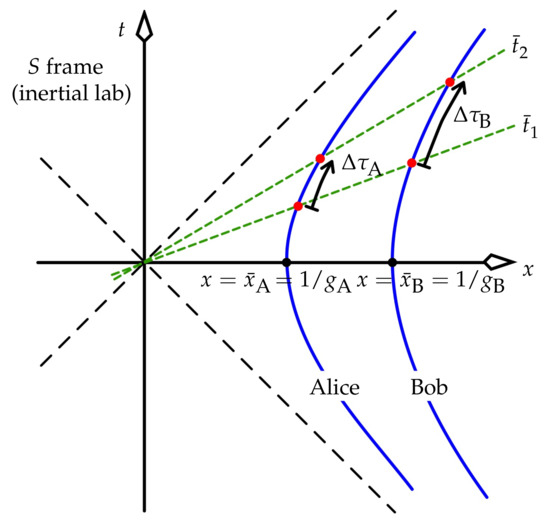
Figure 4.
When Alice and Bob’s shared coordinate time increases from to , Alice ages by and Bob by .
4.5. The Twin Paradox and the UAF
As discussed at length by Good [23], the above prediction of differential ageing that rests on MCIFs and the clock postulate is compatible with the standard resolution of the special relativity’s “twin paradox”.
In Figure 5, consider Alice who stays on Earth, which for the purpose of description we take to be an inertial frame. Her twin brother Bob boards a rocket to a distant star, and later returns to Earth. Bob and Alice agree that when they are reunited, Bob will be younger than Alice because his world line’s integrated proper time is less than the corresponding proper time on Alice’s world line. The paradox results from asking “Cannot each say that the other went on a journey, and therefore each should be younger than the other when they reunite?”. The well-known answer is that “all moving clocks tick slowly” can be stated by inertial Alice, and by Bob if he moves at constant velocity, but not when he is accelerating.
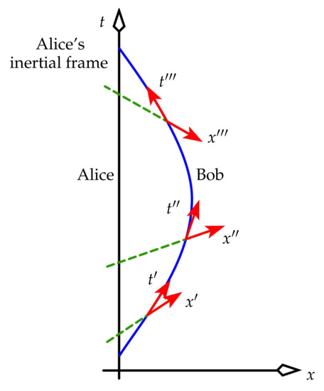
Figure 5.
Bob travels with a constant acceleration in Alice’s inertial frame. At each event on his world line, we draw the space and time axes of his MCIF in the same way as in Figure 1.
Figure 5 shows how the intersection of an always-accelerating Bob’s lines of simultaneity (dashed green) with Alice’s world line (the t axis) gives the age that Bob says “Alice is now”. (The same could be done for Alice: her lines of simultaneity, not shown, are horizontal at each event.)
The scenario usually has Bob accelerate for negligibly small periods of time, outside of which he holds a constant velocity. If Bob were to fly two constant-velocity legs, a pedagogical problem would occur when he jumped from his outbound inertial frame to his inbound inertial frame at his turn-around: the intersection of his line of simultaneity with Alice’s world line would then jump forward discontinuously. The scenario is made more realistic by having Bob accelerate continuously throughout his trip. His world line then has no sharp corners, and so his line of simultaneity never jumps discontinuously: instead, it rotates upwards smoothly in Figure 5. In particular, Bob measures Alice to be
- (1)
- first ageing slowly as his line of simultaneity slides up Earth’s t-axis (Alice’s world line) in a mostly translational way;
- (2)
- then ageing quickly as he slows, and his line of simultaneity begins to rotate and sweep rapidly over Alice’s world line;
- (3)
- then finally ageing slowly as he nears Earth, and the sweep of the simultaneity line is again mostly translational.
Inertial Alice says that Bob always ages slowly only by his instantaneous gamma factor, as decreed by the clock postulate. In Bob’s frame, he is at rest, and Alice has apparently been given a strong push “upwards”. He says that immediately after her departure she ages slowly, corresponding to the first item several lines up. As Alice ascends higher in Bob’s accelerated frame, Bob notes that time at Alice’s location runs faster: her age increases dramatically (corresponding to the second item above). When she descends back to him, she ages slowly once more (corresponding to the third item). Bob’s perception of Alice’s ageing embodies the idea that time runs faster “higher up” in an accelerated frame. The equivalence principle then takes over to predict that time runs faster higher up in a static gravitational field.
Two comments are pertinent here. The first is that no logical problem would arise were Bob to move back and forth for some part of his trip. His line of simultaneity would then see-saw, allowing him to say that Alice’s age was bouncing back and forth, as discussed in Section 3; but no contradiction results from this. This situation is labelled as contradictory in Sections 2 and 3 of [24], which describes two twin scenarios that are both equivalent in our language to Bob accelerating abruptly one or more times during his trip. Ref. [24] effectively writes, in our language, that Bob states Alice’s age to be behaving non-physically, and that Alice has to agree, which Ref. [24] then says is impossible. But this is not how relativity works. Although Bob’s observations are valid, they don’t constrain or interfere with Alice’s evolution. Alice’s age is oscillating for Bob, not for Alice. In a simple analogy, imagine that Bob defined his “line of the horizontal” by the tilt of his head, and then tilted his head back and forth. He would say correctly that Alice’s position was oscillating above and below his horizontal; but that would be of no consequence to Alice, who of course would feel no change in her position.
The above confusion between Alice’s and Bob’s observations as expressed in [24] seems also to have motivated the view in [25]: that reference regards a see-sawing line of simultaneity to be so “wrong” that it concludes no meaning can be given to extending the line arbitrarily far in space. But again, prohibiting the line from being extended arbitrarily is as pointless as preventing Bob from extending his “line of the horizontal” arbitrarily far in space. I have discussed this at length in [26].
The second comment is: it is important to realise that the above difference in rates of flow of time for Alice and Bob is a purely special-relativistic effect, which is then taken on-board general relativity via the equivalence principle. Things are not the other way around. The different rates of flow of time for the twins are often said to result from Bob somehow generating a pseudo gravity field when he accelerates, and supposedly “because GR (general relativity) says that time flows at different rates at different heights in a real gravity field, Bob will say that Alice is ageing faster than him at his turn-around”. This well-worn description puts the cart before the horse. Rather, GR infers that time flows at different rates at different heights in a gravity field via the equivalence principle applied to the special relativity of the UAF. Bob cannot then say that GR is the cause of Alice ageing at a different rate to him. This different ageing rate is naturally consistent with GR; and so GR then lets us deduce what happens to Alice and Bob’s ages in a scenario of real gravity, because that scenario must be consistent (via the equivalence principle) with the pseudo gravity of the twin scenario of this section. But pseudo gravity is purely a useful mental picture. GR should not be treated as the cause of anything in the UAF.
5. Two Speeds of Light in the UAF
In this section, Latin indices denote space coordinates, with summation over repeated indices implied. The coordinate t is a generic “good” time coordinate, by which we mean that all events of constant t are deemed to be simultaneous in the sense of how coordinates are constructed, discussed at the start of Section 4. (See further the discussion of this in Section 7.) The coordinate velocity of a particle is defined as , where the spatial element obeys
In that case,
Suppose that the metric is static (it contains no terms). To calculate the speed of light, , we set between emission and reception events:
Combining (31) and (32) gives
The speed of light is then
If we interpret as the frame’s “rate of flow of time”, then the speed of light equals the rate of flow of time.
In the barred coordinates of the UAF, we can now write
This speed equals zero at the horizon (), as we might expect. It equals 1 (the usual value in an inertial frame) at the location of the master observer (), and increases higher up (larger ). This higher speed results from the global line simultaneity in the UAF rotating in the lab frame as per Figure 3, and hence sweeping over a higher observer’s world line faster than it sweeps over a lower observer’s world line. We interpret this to mean that time flows more quickly higher up, since higher observers age more in a unit of coordinate time than do lower observers—and all observers agree on this because the standard of simultaneity is global to the frame. With time passing more quickly higher up, light must cover more distance per unit coordinate time higher up than it does lower down. (The same argument explains why light’s speed reduces toward the horizon.)
The master observer says that the speed of local light equals 1, and the speed of distant light differs from 1. But any observer can consider himself to be the master, provided he redefines the UAF’s coordinates to suit. This means that all observers in the UAF measure the speed of local light to be 1. This is expected because, by the clock postulate, that speed must equal the speed measured by the MCIF of any observer; and that MCIF, being inertial, measures a speed of 1. Picture a UAF observer having a (brief) conversation with the observer in his MCIF who is momentarily at rest right next to him, and both measuring the speed of light on a table in front of them: by the clock postulate, they must agree on the result. They will not agree on the speed of distant light, and this shows that the UAF is more than just a collection of MCIFs. But that is okay because neither observer can measure the speed of distant light in an experiment, and so they can have nothing to argue about. Accelerated observers thus always measure light’s speed locally to have the familiar value found in an inertial frame. By the equivalence principle, this is also true in a real gravity field.
Additionally, we can define a new velocity , where is the age increase of an observer who is local to the particle. The expression equivalent to (31) is
When the observer is at rest, , and (36) becomes
In particular, for light, we obtain
Thus, the observer always measures this speed of local light to be 1. This is consistent with the clock postulate.
The fact that accelerated observers say that a distant light ray’s speed depends on its location tells us something about the Sagnac Effect. This effect describes the measured difference in the speeds of two light pulses that are sent simultaneously around Earth from one emitter that is fixed to Earth. If the pulses are sent east- and westbound around the Equator, then the westbound pulse will arrive back at the emitter about half a microsecond before the eastbound pulse does. This is, of course, due to Earth rotating in the Solar System inertial frame in which the two pulses have equal speeds. An observer fixed anywhere on the Equator will measure each pulse’s coordinate speed to be 1 as it races past; but when MCIFs are used to analyse the scenario, we find that all such observers say that the coordinate speed is a non-trivial function of the pulse’s longitude and direction of travel. I discussed this at length in [16].
6. Redshift in the UAF
The redshift that Bob observes in a light ray sent to him by Alice can be calculated by following the emission and reception times of two rays, in Figure 6.
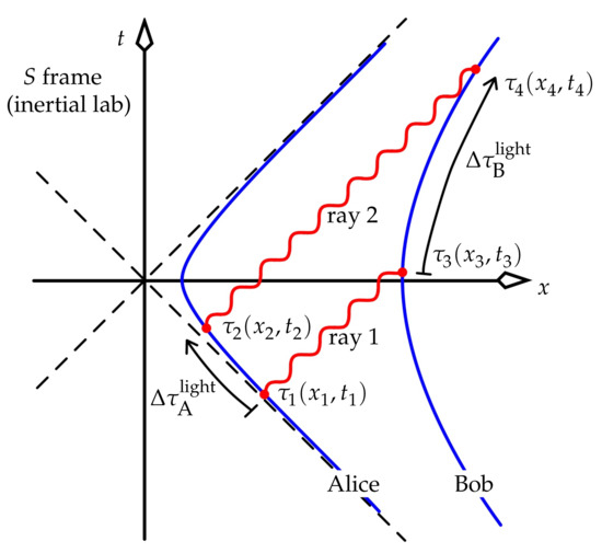
Figure 6.
Alice sends Bob two light rays. These can just as well be envisaged as successive crests of a single light wave.
These can be individual rays, or successive crests of one wave. From the discussion in Section 4.1, a line of simultaneity drawn through the event of Alice emitting a wave intersects Bob’s world line at an event where Bob has the lab velocity that Alice had at the emission event. It follows that, when Bob receives the ray, his rightward velocity in the lab frame is greater than Alice’s velocity was when she emitted the ray. Hence, Bob will measure the light to be redshifted. This is purely a kinematic Doppler shift in the lab; but because Bob says that his separation from Alice is fixed, for him it is not a kinematic effect. He says that seeing and observing are the same in this case, and so the redshift is a consequence of Alice’s time running slower than his time.
A highly simplified version of this section’s calculation was given by Feynman in his lectures [27], and can be found elsewhere in the literature. Feynman studied an accelerating rocket in an inertial lab frame in flat spacetime, and gave all parts of the rocket equal accelerations. Clocks fixed to such a rocket would always have equal speeds in the inertial lab, and so would tick at equal rates. In contrast, Feynman did not explain why the clock at the base of the accelerating rocket in his Figure 42-16 is drawn in the lab as ticking slower, incongruously, than the clock at its head. Feynman’s rocket was not a UAF, but in his simplified calculation, such details as simultaneity and the need for different accelerations were ignored. Although his Doppler calculation was valid, his rocket’s non-UAF-like acceleration would make its inhabitants disagree on simultaneity, and they would thus measure its length to be changing. Hence, they would state that a kinematic Doppler shift was present, and so Feynman’s argument that what they observe is what they see would be invalid. To have the inhabitants say that no kinematic Doppler was present because the rocket’s length was not changing for them (and hence conclude that what they observe is what they see), the rocket would have to be uniformly accelerated. In that case, the clock in the rocket’s base (Alice in our Figure 6) would tick faster than the head clock (Bob) because, at any lab moment, Alice would be moving faster in the inertial lab than Bob. This difference in Alice’s and Bob’s accelerations is, indeed, the origin of the Lorentz contraction. See my comment on Bell’s rockets at the end of Section 4.1.
To calculate the redshift in the UAF, place Alice as usual at , and Bob at . Alice sends two light rays to Bob when she is aged and ; he receives these when he is aged and respectively. How is related to ?
Following (9), we write
In Figure 6, ray 1 is a straight line of slope 1 and passes through , and thus has equation , or
This intersects Bob’s hyperbola at , when Bob is aged . This hyperbola has equation
We will solve (40) and (41) simultaneously for , and then use (39) to solve for . First, write (40) for as
Substitute this last expression into (41), and solve for to give
Because the sinh function is one to one, the inverse sinh can be taken trivially of the left- and right-hand terms in (44), yielding
This is the sought-after expression for . Similarly, we can immediately write down the corresponding expression for ray 2:
We conclude that
In other words,
We can convert (48) to the language of frequency. Alice and Bob agree on the number of rays—or the number of periods of a single wave—that Alice sends to Bob. Alice generates and emits a proper frequency , denoting a number of waves or periods per unit of her proper time: we must use proper time here because Alice’s light generator knows nothing about how her clock might be geared; she might simply have switched on a light bulb. Bob receives and detects a proper frequency , a number of waves or periods per unit of his proper time.5 The number of rays or periods sent from Alice to Bob is then
Equation (49) says
As predicted, Bob sees a redshift that is independent of time, as we might expect. He also observes the same redshift because he says that Alice is not moving relative to himself, and so therefore in his and Alice’s frame (the UAF), the redshift can have no kinematical Doppler component. Realise that Bob doesn’t just see a redshift in the frequency of light emitted by Alice; he also sees all of Alice’s actions passing at the slower rate of (50). But now notice that this redshift factor, or rather its reciprocal , is precisely the rate at which Bob was shown to age faster than Alice in (29).
If, say, Bob is twice as far from the horizon as Alice (), then not only is Alice ageing half as quickly as Bob, but Bob actually sees Alice ageing at half his own rate. While he has 10 birthdays, he sees her have five birthdays. In addition, conversely, Alice will see Bob ageing twice as quickly as herself. Each observer sees the other ageing at a different rate, and, because they have no relative motion in the UAF, they conclude that they are seeing reality, and not some kinematical Doppler artifact: what they observe is what they see. The difference in the flow of time at their different locations is a visible, tangible, effect, and is not something abstract that appears only in a bookkeeping ledger of emission and reception times.
Books on general relativity sometimes describe the different rates of flow of time at different locations in a way that can suggest it is not real, such as: “Bob’s clock appears to tick more quickly than Alice’s clock”. Does the word “appears” (used in [28]) denote a visual appearance? More likely, is it meant to suggest that the “appearance” of different rates of flow of time is not real? Or perhaps that something obscure isn’t being accounted for? Are the clocks displaying proper time (thus showing the ageing of Alice and Bob), or have they been geared to display coordinate time? The UAF teaches us that the different perceived rates of flow of time (different ageings of Alice and Bob) are real. Alice and Bob can quite literally watch each other ageing at a different rate to themselves. In addition, remember that with no relative motion in the UAF to produce a Doppler shift that is only a “trick of the light”, each observer concludes that what they see is what they observe: it is reality.
The agreement of the redshift calculation in this section with the “rate of flow of time” calculations in Section 4 provides a very strong support and validation for analysing the UAF using ideas of simultaneity and MCIFs. This should be kept in mind when these ideas are extended to scenarios in which a frame cannot be defined according to the two rules in Section 4. Such scenarios include rotation in flat spacetime, and curved spacetime; in both of these, the speed of light and the rate of flow of time depends on location. That means the standard special-relativity radar-style procedure of synchronising clocks does not apply, and so ideas of simultaneity lose their standard special-relativity meaning.
7. Scenario Plots in UAF Coordinates
Previously, we drew our spacetime scenarios using the inertial frame’s coordinates . Insight can be gained by picturing the same scenarios in the UAF’s coordinates . First, we make the following observations.
- In Figure 4, and are the spacetime lengths of segments of world lines (that is, how much Alice and Bob age on those segments), whose start events are simultaneous for Alice and Bob, and whose end events are simultaneous likewise, thus defining start and end coordinate times . Equation (29) says that between any two such coordinate times, the age increases of Alice and Bob have the ratio
The fact that here means that Bob receives a period of a wave emitted by Alice over a greater proper time—a greater number of Bob’s heartbeats so to speak—than Bob counts for a period of light that was generated in his vicinity using the same mechanism that Alice used. That is, he sees (and observes) Alice’s light redshifted.
Figure 4 shows the age increases of Alice and Bob for the lapse of a coordinate time . It was drawn in the coordinates of the inertial lab. When it is redrawn in the barred coordinates of the UAF, Figure 7 results.
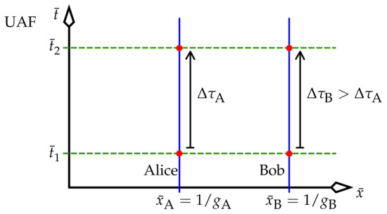
Figure 7.
The scenario of Figure 4 shown in the UAF’s barred coordinates.
Analysing the rate of flow of time consists of finding and comparing the proper time intervals that correspond to a single lapse of coordinate time . We did that in (29), repeated in (51).
It stands to reason that we should be able to draw this figure. The coordinate time is a global standard of simultaneity for the UAF in the same way that an inertial frame has a global standard of simultaneity; hence, we expect to be able to draw spacetime in the UAF such that lines of simultaneity are horizontal, and all vertical distances of the same length on the figure represent the same elapsed coordinate time . That is, after all, what we do without a moment’s thought for inertial frames.
Likewise, Figure 6 drew the redshift in lab coordinates. To redraw it in UAF coordinates, we first ask the question: how are the coordinate time intervals and related, where is the UAF time of event in Figure 6 (and similarly for to )? It turns out that , which we can show as follows.
Extract from the metric (20) the fact that at a fixed , we have , or
Write and . Then, (54) says
Equation (54) also says
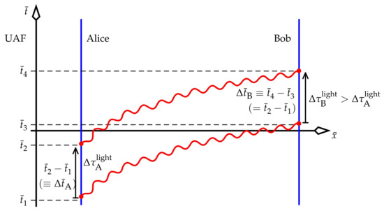
Figure 8.
The scenario of Figure 6 represented in the UAF’s barred coordinates. The light rays’ world lines are drawn curved because the coordinate speed of light is proportional to , as in (35). Note that, although and both refer to the time separation of the two emissions of the rays, they are not necessarily equal; the first is coordinate time and the second is proper time. The same can be said for and .
Again, this figure is reasonable. Because the metric (20) is time independent, we expect that the world line of the second emitted ray in Figure 8 should be a copy of the first emitted ray, translated upward. Hence, it must follow that . To study this time-independence of the metric in more detail, consider calculating , the coordinate time taken for light to travel from Alice to Bob. We set the metric (20) equal to zero: this gives a quadratic equation in which can be solved in terms of spatial infinitesimals and the metric coefficients. Because the UAF’s metric coefficients are time independent, the coordinate-time duration of the transit, , is independent of coordinate time. It follows that the duration of coordinate time between successive emissions of light signals by Alice () equals the duration of coordinate time between successive receptions of those signals by Bob ().
Analysing the redshift consists of finding and comparing the proper time intervals that correspond to the coordinate time intervals , respectively. We wrote the ratio of these proper time intervals in (53).
Thus, Figure 7 and Figure 8 (and equivalently, Figure 4 and Figure 6) both show the proper times that elapse during a single coordinate time interval. This sheds light on the fact that the relevant ratios of elapsed proper times ( and ) are equal [see (53)]. That is, although Figure 7 and Figure 8 show two distinct scenarios, the ratios of proper times elapsed in them are equal. For example, if Bob sees a redshift such that the frequency of Alice’s light is halved [and hence its period is doubled: , as in (50)], then he also knows that he is ageing twice as fast as Alice (). As we have noted previously, what Bob sees is also what he observes: he quite literally sees Alice’s light oscillating in slow motion, and similarly he sees Alice ageing slower than himself. He knows that this is not the result of a Doppler shift in his and Alice’s frame because, in their frame (the UAF), they keep a constant separation.
An assumption of this equality of ageing and redshift might play a role in some standard analyses of the literature, which run as follows. At a fixed location for a given metric, the increment in proper time is (where the time coordinate t is a generic symbol for that used in the frame of interest: it actually corresponds to above). If the metric is time independent, this expression becomes . A ratio of two proper times is then written as
Because this matches the correct expression (53), the redshift result is considered proved and the case pronounced closed. But the reader is left wondering: what has all of this to do with the emission and reception of light rays (or successive crests of a single wave)? And why is the same coordinate time interval used top and bottom in (57)?
We saw in the preceding analysis around Figure 8 and (56) that, in the UAF, the lapse of coordinate time between emissions of the two rays, , turns out to equal the lapse of coordinate time between receptions of the rays, . Hence we can certainly write, for Figure 8,
just as we wrote in (53). But showing that required some work involving the UAF, in (56). It is not obvious a priori. In addition, the “nice” behaviour of the coordinate time here is no doubt due to the fact that it is a bona fide time coordinate, one that obeys the strong requirement for simultaneity at the start of Section 4. It is not clear that such nice behaviour will result from a time coordinate used in, say, Schwarzschild spacetime, where a notion of simultaneity is no longer clear.6 See more discussion of this in Section 10.1 and Section 10.2.
One final note: we saw in Figure 8 that the coordinate times are equal: , and that the proper times are not equal: . These relations seem to have been unknown to Rice, who in the first of two questions put to Eddington in a letter to Nature [29] assumed that the coordinate time intervals for that scenario are not equal, and the proper time intervals are equal. Eddington argued the reverse in his reply, in agreement with what we showed in Figure 8. In Section 2 of [5], Earman and Glymour stated that Rice’s preference for equating proper times was correct; presumably they based this on their belief that coordinates have no strong connection to physical events. But such a belief is incorrect. Yes, arbitrarily defined coordinates can certainly be badly behaved—which is precisely why we were careful to define a “good” time coordinate at the start of Section 4. That section’s construction ensured that is a good time coordinate for the UAF because does have a strong connection to physical events.
I think the distinction between a “good” time coordinate and any arbitrary time coordinate is treated poorly in relativity—if it’s discussed at all. A lack of awareness of this distinction seems central to the unwillingness of some specialists to assign the coordinate time any important role. Studies such as [30] redefine simultaneity in any way that can eliminate some perceived difficulty. We would do better by treating time less cavalierly. In addition, relativity textbooks generally assume that tensor notation puts all coordinates on an equal footing, from which it supposedly follows that one coordinate is no more physically meaningful than another. But tensor notation says no such thing. It allows us to express laws in a coordinate-independent form mathematically; but that does not imply that all coordinates stand on the same footing physically. Reiterating my comments in Section 4, if all coordinates were equally valid physically, then we would have no need to construct “primed coordinates” when discussing “unprimed and primed” inertial frames in introductory relativity textbooks, and the Lorentz transform would have no physical importance. Clearly, relativity has taught us otherwise.
This distinction between good and bad coordinates has been with us since the early days of cartography. Like relativity, any calculations done in cartography require coordinates. Any arbitrary coordinate pair that satisfies a few mathematical constraints is valid to describe a location on Earth; and yet, clearly, some coordinates are better than others. If cartographic coordinates had no meaning beyond being arbitrary labels for locations on Earth, one might invent a new type of latitude/longitude pair such that the curves of constant latitude and constant longitude were not circles and ellipses, respectively, but were some complicated curves of arbitrary shape. This would be a mathematically valid set of coordinates that we could use to allocate two unique numbers to any point on Earth; but it would almost certainly be useless—what I have called a bad set of coordinates—because, for example, it might be thoroughly misleading and extremely difficult to apply to real-world tasks of cartography.
Despite Rice’s early questioning of Eddington’s work, in his own later textbook on relativity, Rice presented Eddington’s analysis as the correct one [5]. Apparently, redshift analyses have been a source of confusion since the beginning. More of this confusion is described in the next section.
7.1. Failure of Schild’s Argument for Curved Spacetime
Several textbooks [6,13,27,28] present an old argument due to Schild that concludes that the existence of redshift implies that spacetime must be curved. (Schild mentions this implication in [31].)
This argument can be formulated for Figure 8 in the following way. It says, correctly, that the existence of a redshift ( in the figure) implies that a different standard of spacetime length () applies to Bob’s world line than to Alice’s world line. Hence, supposedly, the (pseudo-)parallelogram with two curved (red) sides that links the four red dots in that figure cannot be a parallelogram after all (it cannot have two pairs of parallel sides); thus, the spacetime must be curved. The problem with this argument is that the UAF’s spacetime is flat! The above (correct) inequality results from the UAF’s non-Minkowski metric (20), along with the fact that it concerns proper time, whereas the time axis of Figure 8 is coordinate time. Thus, Schild’s argument is invalid; it is a simple case of misinterpreting a non-Minkowski metric in flat spacetime as implying curvature. An increment in proper time can certainly vary with position, and that is precisely what a non-trivial metric encodes. But it does not follow that curvature must be present. In a spatial analogy, Figure 9 shows that the metric for polar coordinates on a flat plane in two-dimensional space is position dependent: . It follows that , but the space is certainly not curved. Compare that figure with Figure 7.
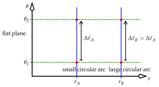
Figure 9.
The flat plane of two-dimensional space in polar coordinates , drawn analogously to the spacetime of Figure 7. Two circular arcs, both centred on the origin , become the blue straight lines in this figure. The metric that describes a length in space is position dependent: . Certainly (the outer arc is longer than the inner arc), but we cannot use that to conclude that the space is curved.
Feynman invoked Schild’s argument in his Lectures on Physics [27]. Naturally, we cannot know if he was over-simplifying his thoughts for his undergraduate target audience. He described a rocket accelerating in what is surely, from the context, flat spacetime. Next, he produced a simplified version of our argument in Section 6, which was valid because his rocket was small. He then used the equivalence principle to transfer his results to real gravity.7 Schild’s argument appeared in his Section 42-7. At the start of that section, Feynman’s text has “We have already pointed out that if the time goes at different rates at different places, it is analogous to the curved space of the hot plate. But it is more than an analogy; it means that space-time is curved”. Feynman immediately went on to draw his Figure 42-18, which is essentially identical to our Figure 7. Corresponding to in our figure, he concluded that the larger value of higher up in his figure implied that its spacetime must be curved. The problem here is that, although his figure ostensibly depicts gravity (that is, curved spacetime), it is also a correct depiction of the UAF’s flat spacetime. Thus, his argument can be interpreted as saying that the flat spacetime of the UAF is curved; a contradiction because a spacetime that is flat for one observer is flat for all observers. It is the Schild-argument flaw of thinking that a non-trivial metric in flat spacetime implies curvature.
Although Feynman placed his scenario in free space, Carroll, Misner et al., and Schutz [6,13,28] placed theirs on Earth’s surface. An observer on Earth is not accelerating in an inertial frame in the same explicit way that Feynman’s rocket occupant was, and this might have some bearing on how these authors phrase Schild’s argument. Schutz and Carroll refer to coordinate time directly in their discussion without drawing any relationship to proper time; Misner et al. make a point of saying that coordinate time equals proper time in their putative inertial frame. It might be said that the coordinate and proper times are equal in the presumed-existing inertial frame; but a discussion that does not distinguish one time from the other can never shed light on the confusion between these times that played a key role in the arguments presented to Eddington by his detractors.
That Schild’s argument is used by so many authors might be due to our familiarity with Mercator maps of Earth’s surface, which really is curved. When we look at such a map, we are aware that the horizontal lines are not what they seem; they are circles of constant latitude. The circumferences of these circles shrink near the poles, even though the lines’ lengths are all equal on the map. Earth’s curvature is the cause, but it is not correct to infer the other way. That is, Earth’s curvature produces this distortion, but not all such distortions are caused by curvature. This is proved by the flat-plane example in Figure 9, the space-only analogy of Figure 7. What would Feynman have made of our Figure 9?8 We can suppose one thing: despite what he and all of the above authors have written, they would all be well aware that determining curvature requires knowledge of the Riemann tensor, and is not necessarily a by-product of a non-trivial metric.
The invalidity of Schild’s argument has been pointed out by Hamilton [11], who stressed the correct roles of proper and coordinate time as presented in our previous sections (but perhaps the details of those roles were obscured by the mass of other results in his paper); and by Marsh and Nissim-Sabat [32], who didn’t stress the correct roles. Brown and Read [10] have also argued that Schild’s analysis is incorrect.
8. Revisiting the Analyses of Eddington and Earman–Glymour
We are now in a position to describe more fully the analyses of Eddington and of Earman and Glymour. Their scenario took place in a real gravitational field; but we are creating a “toy” version of that field by using a UAF. It will be crucial to recall that in Section 7 we showed that the coordinate time elapsing between successive emissions of light signals by Alice equals the coordinate time elapsing between successive receptions of those light signals by Bob.
8.1. Eddington’s Analysis
Eddington’s scenario, placed in a UAF, is shown in Figure 10.
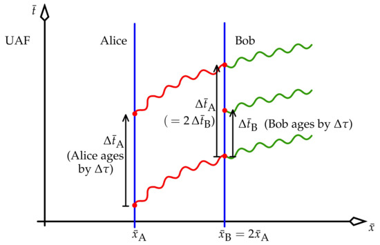
Figure 10.
Eddington’s correct calculation of the redshift. He compared the lapses in coordinate time () for one given proper time elapsing for both Alice and Bob. Alice and Bob’s clocks are identical: they both have the same proper period of ; but Bob ages twice as fast than Alice, and so he ages in half the coordinate time taken by Alice. If, like Alice, Bob sent a light ray upwards at each tick of his clock (), he would emit twice as many light rays as does Alice per unit coordinate time, as shown in green.
He compared the lapses in coordinate time () for one given proper time elapsing for both Alice and Bob. For the sake of argument, place Bob twice as far from the horizon as Alice: . Alice’s clock ticks once every , equivalent to a proper time for Alice. That is, Alice ages by between ticks of her clock, and so the metric says that
She sends a light ray to Bob at each tick. Bob receives these tick signals at intervals of the same quantity, , as we recalled in the previous paragraph. Bob’s clock ticks at intervals of , which need not equal ; this depends on how the coordinate time was defined. But the clocks were manufactured identically, and so Bob ages by the same proper time between his clock’s ticks as does Alice between her clock’s ticks. The metric then says that
If Bob sent his own light ray upwards at each tick of his clock (), he would emit twice as many rays as does Alice per unit coordinate time. These hypothetical rays are drawn green in Figure 10.
In particular, since we have set , we see from (59) and (60) that
In this case, Bob receives Alice’s signals at half the rate of his own ticking. That is, Bob sees Alice’s clock to be ticking slow by the factor , or half of his clock’s rate: he sees her ageing in slow motion. Bob also observes the same result because he knows that Alice is not moving relative to him in their shared frame (the UAF), and so no kinematical Doppler shift can be present. This is Eddington’s analysis of the redshift in our language, and it is perfectly valid.
8.2. Earman and Glymour’s Analysis
Earman and Glymour’s scenario is shown in Figure 11.
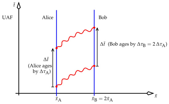
Figure 11.
Earman and Glymour’s correct calculation of the redshift. They compared the lapses in proper time () for one given coordinate time elapsing for both Alice and Bob.
They compared the lapses in proper time () for one given coordinate time elapsing for both Alice and Bob. (Our description of their analysis in Section 2 used a generic time coordinate t, but we now specifically use the UAF coordinate .) Alice and Bob have identical clocks. As usual, the proper period of these clocks is the time that each observer ages in one period of their own clock. In particular, focus on Alice, and call this period . (Bob ages by the same amount, , in one period of his clock.) Alice’s clock’s period also corresponds to a coordinate time . This is not the coordinate period that Bob ascribes to his clock. But it is the period that Bob sees and observes between Alice’s ticks.
9. Difficulty with the Energy-Plus-Quantum Argument for Redshift
We saw in Figure 8, Figure 9, Figure 10 and Figure 11 that a light ray’s coordinate frequency (number of oscillations per unit coordinate time ) does not drop en route from Alice to Bob, but its proper frequency (number of oscillations per unit personal proper time ) certainly does drop from Alice to Bob.
The proper frequencies are most naturally measured: they do not depend on any clock gearings, and so, in a manner of speaking, answer Alice’s question “How many cycles of the light were emitted per each of my heart beats?” and Bob’s question “How many cycles of the light were received per each of my heart beats?”. But the coordinate frequency also has real physical meaning because the UAF’s coordinate time has physical meaning. The coordinate time defines a global standard of simultaneity for the frame, and hence is a privileged choice of time for the UAF.
We should take seriously, then, the idea that the coordinate frequency does not drop in the UAF en route from Alice to Bob, and hence that the difference in proper frequencies measured by Alice and Bob is not due to something happening to the travelling light, but to the twins ageing at different rates. This is reasonable; after all, by what mechanism could such a drop occur in any static scenario if Alice and Bob were ageing at the same rate? It would require successive crests to take longer and longer to travel from Alice to Bob; but light’s speed cannot be time dependent in a static scenario. This was already realised by Einstein some years before general relativity came about [5], and forced him to conclude that Bob must really be ageing faster than Alice in the context of true gravity.
Now, consider a basic exercise in non-relativistic classical mechanics: say, computing the trajectory of a projectile in a uniform gravitational field. The scenario occurs in a non-inertial frame; but if we are to apply Newton’s equations of motion (which apply only to inertial frames), we model the frame as being inertial with a “gravity force” present. This idea might be applied to the light that Alice sends to Bob. Suppose they model their frame as inertial with a “gravity force” present. In that case, because Alice and Bob are at rest, each writes their metric as “”, meaning proper and coordinate times are equal, and hence proper and coordinate frequencies are equal. We can compute the redshift with what is a standard argument in the literature, as follows.
Alice generates a light ray of energy E. She sends this up the gravitational potential . The ray loses energy and is received by Bob. The value of can be determined by energy conservation with the following thought experiment. Bob converts the light of energy into a mass (where we retain factors of c to highlight the use of mass here). We assume he can do this with full efficiency, barring any known Carnot-type argument to the contrary. He then drops this mass back down to Alice. For a weak field (), we can omit the momentum-conserving back-reaction of the mass’s motion on the field, and simply say that the mass gains kinetic energy . Alice converts the mass and its kinetic energy back into a light wave of energy
Energy conservation says this should equal E. It follows that
Setting again for conciseness, we conclude that, whereas Alice emits light of energy E, Bob receives light of energy . We now take a photon view and write “” with h Planck’s constant. Re-use the in (49): Alice emits light with a frequency that she measures to be , and Bob receives that light and measures its frequency as , where
Equation (66) is the standard redshift expression, validated by experiment. It matches the expression we derived in (50). The reason is that (50) can be written as
and because [as mentioned just after (2), but now in barred coordinates] for a weak static gravitational potential, it follows that
We can also argue that light must lose energy in climbing a gravitational field by considering a mass m at sea level that is converted with 100% efficiency to light. This light is sent upward, received, and converted back to mass. That mass must be less than m, since otherwise we would have sent the mass upwards at no energy cost. On the other hand, if the 100% efficiency cannot be attained, it might imply the existence of some type of Carnot theorem for converting mass to energy; but no such theorem is known.
The thought experiment preceding (64) can be eliminated by positing that light of energy E has a relativistic mass of . This mass is reduced by as the light climbs the potential, bringing us to (65) immediately. In non-relativistic mechanics, a particle that is shot upwards in a gravitational field has its kinetic energy converted to potential energy while its mass stays fixed. But in relativity, the particle’s kinetic energy contributes to its relativistic mass; hence, the particle’s relativistic mass is reduced as the particle ascends. The same idea holds for light here: the loss in relativistic mass of the ascending light means that its energy is reduced from E to .
This simplified derivation—that avoids transforming energy to mass and vice versa—has been questioned by Earman and Glymour [5], and pronounced invalid by Okun et al. [14]. These authors object to light obeying what Okun calls a non-relativistic analysis built around an energy loss of . Okun goes further, pronouncing incorrect Einstein’s 1911 statement “whenever there is mass, there is also energy and vice versa”, on the basis that the photon has no (rest) mass. But light’s zero rest mass is irrelevant here. Light clearly has energy, and it is reasonable to imagine transforming that energy into mass in the thought experiment preceding (64) where that mass was dropped back down to Alice. Thus, nothing here negates Einstein’s statement, and the relativistic-mass view is a conveniently brief way to present the thought experiment of converting between light and mass.9
Nonetheless, the redshift cannot be a coordinate-frequency drop between observers who age at the same rate, because the very idea that a signal’s coordinate frequency can change from emission to reception in the static case where emitter and receiver are ageing at the same rate and have no relative motion makes no logical sense: the frequency drop would imply successive wave fronts were taking longer and longer to reach Bob, contradicting the fact that the signal’s speed was time independent. Hence, we must interpret the redshift as due to Bob ageing faster than Alice, and not to any drop in coordinate frequency happening en route from Alice to Bob. Recall the comment just after (48): proper frequency is the relevant quantity here, and Bob’s measurement of it is less than Alice’s because he is ageing faster than her. The “f” in Planck’s identity “” is the observer’s proper frequency, not coordinate frequency. When we invoke that identity, we are already unconsciously allowing Alice and Bob to age at different rates. Planck’s identity goes hand in hand with the idea that time flows differently at different heights in an accelerated frame or gravity field.
Even though light’s coordinate frequency does not drop as it ascends the potential that is present in the UAF, it does not ascend for free, with no energy price being paid. What we might call an energy price is reflected in the different rates of flow of time with height in the UAF. The principle of energy conservation is thus intimately related to the rate of flow of time. This goes beyond Nöther’s theorem, which says that energy conservation results from a system’s dynamics having no time dependence. Nonetheless, it’s clear that defining a gravitational energy becomes problematic in relativity. The ascending light has not given energy to the gravity field; instead, the state of the observer has been central to the description of the light.
The classical loss of mass/energy of a particle that ascends a (real or apparent) gravity field might indicate a relationship of mass to time. When Alice looks up, she sees/observes Bob going about his daily activities in fast motion. If Alice and Bob apply equal forces to identical metal blocks stamped “100 kg” on rollers, Alice marvels that Bob can give his block a higher acceleration than she can give hers. She concludes that if Bob is ageing at the same rate as she, then his block must be less massive than hers. But if she demands that his block have the same mass as hers, then she must conclude that his time is unfolding faster than her time.
10. Redshift in Real Gravity
Given that the UAF approximates (but is not equivalent to) a uniform gravitational field over small distances, the equivalence principle helps us infer at least some behaviour of a real gravitational field from it. For example, we infer that clocks (i.e., time) run faster the higher they sit in a real gravitational field. This prediction is verified daily because it is built in to global satellite navigation systems. Atomic clocks on-board such satellites are “geared down” just as Bob’s clock was in Section 4.2: they are manufactured to “tick” slightly slowly on Earth, so that, when in orbit and ageing (hence ticking) faster than they were in the factory, they tick at the same rate as their counterparts on Earth. This allows the relevant equations for time and position to be solved unambiguously. (This quickening of a satellite’s tick rate upon reaching a typical global navigation orbit is the sum of two contributions: the larger is the rate increase caused by the gravitational potential, and the smaller is a decrease caused by the orbital motion.)
Let’s use the equivalence principle to apply (68) to a real field with gravitational acceleration g. For observers at rest on or near Earth’s surface, kinematic effects due to Earth’s rotation are negligible; then (68) becomes, with factors of c restored,
This formula was tested by the 1960s Mössbauer experiments of Pound, Rebka and Snider. They measured the redshift of gamma rays sent by the equivalent of Alice from an Earth-stationary source up 22.5 metres to an Earth-stationary detector held by the equivalent of Bob. Equation (69) predicts a redshift of
This value agrees with the experimentalists’ findings to a 1% accuracy [34]. Alternatively, we can imagine that the experiment was carried out in a UAF and use the barred coordinates of (67) without discussing gravitational potential at all. Alice and Bob’s “heights” (above the horizon ) are then
with m. Equation (67) says [referring to (70) for the numbers]
This agrees with (69) and (70). The expression has been confirmed over sub-metre values of h by modern precision clocks [35]. Echoing the end of Section 6, this agreement of the UAF/MCIF approach to redshift with experiment forms a strong validation of the whole philosophy of using MCIFs to define simultaneity in an accelerated frame, coupled with the equivalence principle to discuss real gravity.
In his 1960 book [36], Synge suggested dismissing the equivalence principle from modern physics, saying that its role had been only to help general relativity be born, and that it should now be “buried with appropriate honours”. In contrast, we have seen above that the principle is alive and well, and is necessary for introducing the UAF into any modern discussion of gravitational redshift.
10.1. Redshift from the Schwarzschild Metric
How might we reproduce (68) using, say, the Schwarzschild metric, which describes Earth’s gravitational field well for our purposes? The Schwarzschild metric is
Can we use the argument of Section 7 and Figure 8 to derive the redshift, which we know should be at least approximately (68)? The Schwarzschild metric describes a curved spacetime, not the flat one shown in Figure 8. Nevertheless, just as we can draw Earth’s surface with some distortion on a flat page, we should be able at least to envisage depicting Schwarzschild spacetime on a flat page. Any distortion will not affect the static nature of the metric, meaning that successive light rays should appear as in Figure 8; that is, they should all be congruent, irrespective of how their speed might change en route from emitter to receiver. Thus, Figure 8 applies to Schwarzschild spacetime: in particular, the lapses in the coordinate time t of the metric (73) (not proper time !) between successive emissions and between successive receptions should be equal: . This is the crucial point to realise, and once we have it, the rest is easy. We combine (50) with the reciprocal of (58) (using Schwarzschild’s t, not the UAF’s ) to write
For the metric (73), the last term in (74) becomes the of (72).
One big difference is evident between the “” argument as applied to Figure 8 in Section 7, and to Schwarzschild spacetime in the previous paragraph. The UAF time in Figure 8 is a “good” time coordinate: it gives a well-defined global standard of simultaneity to the UAF. But the time t in the Schwarzschild metric doesn’t guarantee any simultaneity at all, local or global. It is the time shown on the master clock located at spatial infinity, but it is not assigned to events in any way that accords with the simultaneity standard present in special relativity. What role this difference in the time coordinates of UAF and Schwarzschild might play in more advanced discussions of redshift and time is not clear.
Aside from that, the discussion in Section 7 shows that ageing and redshift are synonymous in Schwarzschild spacetime. Construct a variant on the usual twin paradox, in which Alice and Bob both fly independently around the world, or perhaps one stays at home. When they meet, what is their age difference ? Their proper times elapsed are each given by integrating the metric (73) over their paths in spacetime. This is easier said than done, because it demands a knowledge of the quantities , , and . For example, if Alice traverses a “small circle” at a fixed height and latitude, then her age increase—her elapsed proper time—is
We might be inclined to say that, to a high approximation, is Alice’s velocity in the Solar System frame in which Earth spins.10 To calculate this velocity, we might be given Alice’s velocity over Earth’s surface, and will have to combine that with Earth’s spin velocity at her latitude. It’s not clear how to do this at a deep level; should the velocities be added special-relativistically? Why? At its core, this question relates to what it means for Alice’s velocity to be specified “over Earth’s surface”, since this involves relativistic rotation, a subject of much debate. Typical experiments use such low speeds that the velocities are added directly. This analysis is at the core of Hafele and Keating’s 1971 experiment, in which clocks were flown around the world. Their results gave a low-speed confirmation of relativity’s current ideas of proper and coordinate times in the Schwarzschild metric.
10.2. A Global Time for Earth
The calculation that produced (69) disregarded Earth’s rotation as negligible. When details of that rotation are included, we find a phenomenon that is used to define our modern global time, called TAI (and dubbed UTC when leap seconds are included.) Earth’s rotation gives it an oblate-spheroid surface. Including gravitational effects from the non-uniform surface distribution of land masses and oceans produces the geoid: a best fit to Earth’s surface, with all of its points at a single effective gravitational potential that combines gravity with rotation.
Alice and Bob are fixed to different points on the geoid. Equation (73) is now modified to include Earth’s spin: is set equal to Earth’s spin rate times . This modifies such that . A superficial comparison of light frequencies in (74) then indicates that a light ray sent by Alice to Bob will be received without being redshifted. (This also follows from the energy-conservation argument in Section 9: the total work done by the light en route from Alice to Bob is zero, and hence Bob measures no change in frequency of the light.) But because Alice and Bob say that they have no relative motion, then (as discussed in Section 6) what they see is reality. They each conclude that the other is ageing at the same rate as themselves. This is the standard argument for all clocks ticking at the same rate on the geoid, without requiring gearing. This rate is called TAI, whose SI unit is the second defined from the physics of the caesium atom.
That said, the above geoid discussion assumes the existence of the time t in (73) and (74). Constructing a meaningful time on a rotating Earth even in the absence of gravity is a delicate procedure, as I have discussed in [16,26]. It turns out that global simultaneity breaks down on a rotating Earth—at least in the absence of gravity—but not for the reason commonly found in papers in the subject, which string together one-space-dimensional Lorentz transforms naïvely. As already stated in Section 10.1, this lack of global simultaneity might cause problems for any discussion of rotation. The last words on that topic have yet to be said. Unfortunately, the precise-timing community remains almost completely unaware of these delicate nuances of the theory.
11. Conclusions
Eddington’s and Einstein’s analysis of redshift lay at the cutting edge of their time; and, although correct (at least as far as a modern interpretation of Eddington’s gravitational argument goes), was not well understood in their day. Perhaps that was partly due to a lack of precision in Eddington’s language. Earman and Glymour [5] say that Eddington wasn’t completely sure of what he wrote. The UAF’s analysis vindicates Eddington and Einstein, while preserving the correctness of the alternative derivation made by their detractors, Earman and Glymour. It also sheds light on the analyses of authors such as Schild. Section 7.1’s discussion of some modern authors suggests that, even today, the roles of proper and coordinate time are not distinguished from each other as well as they should be. That might be a result of the modern practice of redefining time and simultaneity through arbitrary foliations of spacetime—a practice that I think has no deep physical meaning, and only ends up trivialising what is really a rich subject. The UAF approach accomplishes much, while remaining in the comparatively well-understood realm of special relativity. For this, and for what it tells us about real gravity via the equivalence principle, the uniformly accelerated frame deserves a more prominent role in the teaching of relativity.
I thank the referees for their comments, which corrected a couple of mistakes and made some things clearer.
Funding
This research received no external funding.
Conflicts of Interest
The author declares no conflict of interest.
References
- Scott, R.B. Teaching the gravitational redshift: Lessons from the history and philosophy of physics. J. Phys. Conf. Ser. 2015, 600, 012055. [Google Scholar] [CrossRef]
- Eddington, A. Report on the Relativity Theory of Gravitation, 2nd ed.; Fleetwood Press: London, UK, 1920. [Google Scholar]
- Eddington, A. The Mathematical Theory of Relativity; Chelsa: New York, NY, USA, 1975. [Google Scholar]
- Weinberg, S. Gravitation and Cosmology: Principles and Applications of the General Theory of Relativity; John Wiley & Sons: New York, NY, USA, 1972. [Google Scholar]
- Earman, J.; Glymour, C. Studies in History and Philosophy of Science. Stud. Hist. Philos. Sci. 1980, 11, 175–214. [Google Scholar] [CrossRef]
- Misner, C.; Thorne, K.; Wheeler, J. Gravitation; W.H. Freeman: New York, NY, USA, 1973. [Google Scholar]
- Desloge, E.; Philpott, R. Uniformly accelerated reference frames in special relativity. Am. J. Phys. 1987, 55, 252–261. [Google Scholar] [CrossRef]
- Desloge, E. The gravitational red shift in a uniform field. Am. J. Phys. 1990, 57, 856–858. [Google Scholar] [CrossRef]
- Nobili, A.M.; Lucchesi, D.M.; Crosta, M.T.; Shao, M.; Turyshev, S.G.; Catastini, G.; Anselmi, A.; Zavattini, G. On the universality of free fall, the equivalence principle, and the gravitational redshift. Am. J. Phys. 2013, 81, 527–536. [Google Scholar] [CrossRef]
- Brown, H.R.; Read, J. Clarifying possible misconceptions in the foundations of general relativity. Am. J. Phys. 2016, 84, 327–334. [Google Scholar] [CrossRef]
- Hamilton, J.D. The uniformly accelerated reference frame. Am. J. Phys. 1978, 46, 83–89. [Google Scholar] [CrossRef]
- Hughes, R. The Bohr–Einstein “weighing-of-energy” debate and the principle of equivalence. Am. J. Phys. 1990, 58, 826–828. [Google Scholar] [CrossRef]
- Schutz, B. A First Course in General Relativity; Cambridge University Press: Cambridge, UK, 1988; p. 44. [Google Scholar]
- Okun, L.B.; Selivanov, K.G.; Telegdi, V.L. On the interpretation of the redshift in a static gravitational field. Am. J. Phys. 2000, 68, 115–119. [Google Scholar] [CrossRef]
- Cook, R. Physical time and physical space in general relativity. Am. J. Phys. 2004, 72, 214–219. [Google Scholar] [CrossRef]
- Koks, D. Simultaneity on the Rotating Disk. Found. Phys. 2017, 47, 505–531. [Google Scholar] [CrossRef]
- Desloge, E. Nonequivalence of a uniformly accelerating reference frame and a frame at rest in a uniform gravitational field. Am. J. Phys. 1989, 57, 1121–1125. [Google Scholar] [CrossRef]
- Koks, D. Explorations in Mathematical Physics; Springer: New York, NY, USA, 2006; Chapters 7 and 12. [Google Scholar]
- Bailey, J.; Borer, K.; Combley, F.; Drumm, H.; Krienen, F.; Lange, F.; Picasso, E.; Von Ruden, W.; Farley, F.J.M.; Field, J.H.; et al. Measurements of relativistic time dilation for positive and negative muons in a circular orbit. Nature 1977, 268, 301–305. [Google Scholar] [CrossRef]
- Sherwin, C.W. Some Recent Experimental Tests of the “Clock Paradox”. Phys. Rev. 1960, 120, 17–21. [Google Scholar] [CrossRef]
- Rindler, W. Kruskal Space and the Uniformly Accelerated Frame. Am. J. Phys. 1966, 34, 1174–1178. [Google Scholar] [CrossRef]
- Faber, R.L. Differential Geometry and Relativity Theory; Marcel Dekker Inc.: New York, NY, USA, 1983. [Google Scholar]
- Good, H. Uniformly accelerated reference frame and twin paradox. Am. J. Phys. 1982, 50, 232–238. [Google Scholar] [CrossRef]
- Kholmetskii, A.L. The Twin Paradox in Special Relativity and in Lorentz Ether Theory. Apeiron 2003, 10, 204–230. [Google Scholar]
- Mermin, N.D. It’s about Time: Understanding Einstein’s Relativity; Princeton University Press: Princeton, NJ, USA, 2005. [Google Scholar]
- Koks, D. Simultaneity and Precise Time in Rotation. Universe 2019, 5, 226. [Google Scholar] [CrossRef]
- Feynman, R.P.; Leighton, R.B.; Sands, M. The Feynman Lectures on Physics; Vol. II, Sections 42-6 and 42-7; Addison-Wesley: Reading, MA, USA, 1964. [Google Scholar]
- Carroll, S. Spacetime and Geometry: An Introduction to General Relativity; Cambridge University Press: Cambridge, UK, 2019. [Google Scholar]
- Rice, J. The Predicted Shift of the Fraunhofer Lines. Nature 1920, 104, 598–599. [Google Scholar] [CrossRef]
- Cranor, M.; Heider, E.; Price, R. A circular twin paradox. Am. J. Phys. 2000, 68, 1016–1020. [Google Scholar] [CrossRef]
- Schild, A. Equivalence Principle and Red-Shift Measurements. Am. J. Phys. 1960, 28, 778–780. [Google Scholar] [CrossRef]
- Marsh, G.E.; Nissim-Sabat, C. Does a gravitational red shift necessarily imply space-time curvature? Am. J. Phys. 1975, 43, 266–267. [Google Scholar] [CrossRef]
- Okun, L.B. Reply to the letter “What is mass?” by R.I. Khrapko. Physics–Uspekhi 2000, 43, 1270–1275. [Google Scholar] [CrossRef]
- Pound, R.; Snider, J. Effect of Gravity on Nuclear Resonance. Phys. Rev. Lett. 1964, 13, 539–540. [Google Scholar] [CrossRef]
- Chou, C.W.; Hume, D.B.; Rosenband, T.; Wineland, D.J. Optical Clocks and Relativity. Science 2010, 329, 1630–1633. [Google Scholar] [CrossRef]
- Synge, J.L. Relativity: The General Theory; North-Holland: Amsterdam, The Netherlands, 1960. [Google Scholar]
| 1. | The equivalence principle is formulated in various ways in the literature, and the question of how these are related lies outside this paper. We take the principle to state that over a “small” region of spacetime, the action of a gravity field on any experiment is identical to performing that experiment in an accelerating laboratory in zero gravity. See also the comment just after (21). |
| 2. | Some authors refer to a no-acceleration variant of this with two people walking past each other as the “Andromeda Paradox”. |
| 3. | The MCIF is known in the literature by various names, including instantaneous rest frame and momentarily comoving reference frame. |
| 4. | Despite the UAF approximating the frame in which each of us lives and in which almost all physics experiments are carried out, it does not have a high profile even in advanced relativity courses. |
| 5. | Don’t confuse the here with the of Eddington’s analysis in Section 2. The are frequencies of Eddington’s clocks—which might be local light generated by each observer; but are the emitted and received frequencies of the light sent from Alice to Bob: equal Earman–Glymour’s respectively. |
| 6. | In the usual Kruskal–Szekeres coordinatisation of Schwarzschild spacetime, light cones are drawn just as they are in flat spacetime. Does it follow that Schwarzschild simultaneity is well determined by constant surfaces of the Kruskal–Szekeres time coordinate? That spacetime has a well-defined direction of up/down; but why should simultaneity be determined by a time parameter that renders the light cones symmetrical in the up–down direction? |
| 7. | A crucial point: Feynman’s transcribed words make it unclear whether he distinguished seeing from observing. His text has “But if one [clock] always appears to be running at a different speed with respect to the other [clock], then so far as the first is concerned the other is running at a different rate”. His comment holds only because the clocks in his rocket have no relative motion, and hence no kinematic Doppler shift. I might add here that, when discussing moving clocks, I think it’s best to avoid words such as “running” and “speed”; these are too easily confused with kinematics, instead of the rate of flow of time that they are meant to describe. “Running at a different speed” is better replaced by “Ticking at a different rate”, and we must always remember that a clock’s tick rate really does equate to the rate of flow of time onboard the clock. |
| 8. | I’m sure he would have appreciated the arguments above, since he knew that his Lectures on Physics were not above the occasional hiccup. As an example, consider Feynman’s discussion of the force acting on a capacitor plate in Section 8-2 of his Lectures’ Volume II. When the total field in the capacitor is his value , the force on each plate equals its charge times the field of the other plate, since a plate doesn’t act on itself. Feynman derived this term using an energy argument, and then expressed surprise at the presence of the 1/2. I think that the hindsight explanation he gave for it doesn’t really work: it appeals to an average field strength inside capacitor plates that are required to be macroscopic conductors, belying the idea that the plates should be treatable as thin sheets of charge only, and with no averaging necessary. |
| 9. | In [14], Okun is really expressing his aversion to the concept of relativistic mass, which he expounds on in [33]. But that mass finds a perfect use in simplifying the above valid thought experiment. Light has zero rest mass , in that it satisfies the general particle equation for . Its momentum is . Hence, being multiplied by light’s speed c in an inertial frame, certainly plays the role of a mass. The thought experiment in this section shows that this mass behaves in the way that we expect of a mass that is raised in a gravity field. |
| 10. | My own essay on this in [18] has a typographical error in its equation (12.58) and the sentence immediately following. The terms and should be absent, and the plane’s velocity should be . These typos cancel in (12.58), so that it still returns the correct numbers. |


Publisher’s Note: MDPI stays neutral with regard to jurisdictional claims in published maps and institutional affiliations. |
© 2020 by the author. Licensee MDPI, Basel, Switzerland. This article is an open access article distributed under the terms and conditions of the Creative Commons Attribution (CC BY) license (http://creativecommons.org/licenses/by/4.0/).