Article

Foundations of Finsler Spacetimes from the Observers’ Viewpoint

1
Departamento de Geometría y Topología, Facultad de Ciencias, Universidad de Granada, Campus Fuentenueva s/n, 18071 Granada, Spain
2
Departamento de Matemáticas, Universidad de Murcia, Campus de Espinardo, 30100 Espinardo, Murcia, Spain
*
Author to whom correspondence should be addressed.
Universe 2020, 6(4), 55; https://doi.org/10.3390/universe6040055
Submission received: 29 February 2020 / Revised: 7 April 2020 / Accepted: 13 April 2020 / Published: 16 April 2020
(This article belongs to the Special Issue Finsler Modification of Classical General Relativity)

Abstract

:
Physical foundations for relativistic spacetimes are revisited in order to check at what extent Finsler spacetimes lie in their framework. Arguments based on inertial observers (as in the foundations of special relativity and classical mechanics) are shown to correspond with a double linear approximation in the measurement of space and time. While general relativity appears by dropping the first linearization, Finsler spacetimes appear by dropping the second one. The classical Ehlers–Pirani–Schild approach is carefully discussed and shown to be compatible with the Lorentz–Finsler case. The precise mathematical definition of Finsler spacetime is discussed by using the space of observers. Special care is taken in some issues such as the fact that a Lorentz–Finsler metric would be physically measurable only on the causal directions for a cone structure, the implications for models of spacetimes of some apparently innocuous hypotheses on differentiability, or the possibilities of measurement of a varying speed of light.

1. Introduction

A plethora of alternatives to classical general relativity has been developed since its very beginning. Many of them were motivated by the search of a unified theory which solved disturbing issues of compatibility with quantum mechanics (Kaluza–Klein, M-theory, quantum field gravity, etc.) while, since the 90s, unexpected cosmological measurements led to further alternatives (cosmological constant, quintaessence, theories with varying speed of light, etc.). However, the possibility to consider a Finslerian modification of General Relativity has not settled in mainstream research, and it has been scarcely considered in the literature until recent times (some examples are References [1,2,3,4,5,6,7,8,9,10,11,12,13,14,15]). Certainly, the generality of Finsler geometry in comparison with the Riemannian setup (namely, analogous to the generality of the convex open subsets of an affine space in comparison with the ellipsoids) is a big drawback, as the number of new variables and parameters would seem immeasurable. Nevertheless, this is similar to the generality of general relativity in comparison with the special one (see Remark 13). Anyway, any Finslerian modification of general relativity would mean to drop the beloved Lorentz invariance not only at global and local levels (as it occurs in general relativity) but also infinitesimally, i.e. looking such an invariance as a limit symmetry around each event. However, from a fundamental viewpoint, this should not seem too strange: as physical measurements are always approximations, one would not be surprised if the symmetries of the models were only approximations to a more complex reality. Indeed, as we will explain, the existence of some symmetries among observers becomes a natural requirement in order to make direct measurements of space and time. There is no reason to assume that the physical reality will satisfy such requirements in an exact way—even though, certainly, the existence of such approximated symmetries are meaningful and useful for modeling.
In the present article, a physical motivation to consider Finsler spacetimes as models of space and time is developed and quite a few of related ideas are discussed. We stress the following four guidelines.

1.1. Approach from the Foundations Viewpoint

We develop an approach for the foundations of the theories of spacetime starting at the observers viewpoint in classical mechanics and special relativity (Section 2, Section 3 and Section 4). Finsler spacetimes are shown to appear by dropping the symmetries of inertial observers in a natural way. Our approach follows the viewpoint in Reference [16] by López and by two of the authors in Section 2 and Section 3, which includes the celebrated ideas by V. Ignatowski [17,18] about the foundations of special relativity.
Specifically, we argue that the geometric models of spacetime appear from the notion of inertial observers by means of a double linearization of the measuring problem, namely,
(1)
there are inertial frames of reference (IFR) in which changes of coordinates are linear, and
(2)
the symmetries in the change of the time-like coordinate (and, independently, in the three spacelike ones) between two IFR’s are encoded in that linear structure.
These assumptions lead to four classic linear 4-dimensional structures, namely Lorentz–Minkowski, Galilei–Newton, dual Galilei–Newton, and Euclidean (see Section 2). Dropping (1) leads from special to general relativity (see Section 3) as well as to other transitions for the other three structures. The latter are also briefly explained here, namely, from Galilean to Leibnizian spacetimes (see Section 3.4), including signature changing metrics (see Section 3.1), and the possibility of a pointwise varying speed of light (see Section 3.3). Dropping (2) leads to Lorentz–Minkowski norms and, then, to Finsler spacetimes, discussed both mathematically and physically in Section 4.

1.2. Critical Revision of EPS Axiomatics

The classical Ehlers, Pirani, and Schild (EPS) approach for general relativity [19,20] will be revisited (see Section 5). We show that, certainly, this approach is compatible with the existence of Lorentz–Finsler metrics, a possibility already suggested by Tavakol and Van Den Bergh for Berwald spaces [15] (see the discussion in Section 5.2.5). Such a possibility was ignored in EPS because of a too restrictive development of two steps1, namely:
  • An artificial requirement of smoothability of some combination of radar coordinates, which would forbid null cone structures incompatible with Lorentzian metrics. This was recently pointed out by Lammërzhal and Perlick’s [11], and it is developed here in detail (see Section 5.2.1).
  • A deduction of the existence of a projective structure starting at a general version of the law of inertia. This would exclude the time-like pregeodesics for a Lorentz–Finsler metric (except those of Berwald-type), but again, the proof crucially relies on an argument of C 2 -differentiability, which is related to nontrivial issues on Finslerian metrics (see Section 5.2.2).

1.3. Precise Geometric Framework

Along the article, a careful mathematical approach is carried out following Reference [10]. For the convenience of the reader, a brief mathematical summary on (Lorentz) Finsler concepts is also included in Section 4.1. This allows us to model and to discuss issues on Lorentz–Finsler metrics L which turn out to be important from the physical viewpoint such as the following:
(1)
Causal cone domain (Section 4). The physically meaningful domain for L is only the causal cone of a cone structure C .
Indeed, even in the classical relativistic case, only the future-directed causal directions for a cone C + determined by the metric g contains the elements physically measurable for any (true or gedanken) experiment. In relativity, the Lorentzian scalar product g p at each event p is determined by its value on the cone C p + (or on its time-like directions); therefore, a Lorentz metric g can be determined on the whole T M even if, actually, only its value on C + can be measured. However, this is not by any means true for a Lorentz–Finsler metric L, where there is a huge freedom to extend the Lorentz–Finsler metric away from C .
Therefore, our Lorentz–Finsler metrics will be defined only on a (causal) cone structure2.
(2)
Smoothness, i.e., differentiability up to some appropriate order. Usually, such a requirement is regarded as a harmless macroscopic approximation to the structure of the spacetime. However, the discussion on EPS above shows that this is not so trivial in the Finslerian case. Furthermore, other issues appear in the literature:
The possibility that the cone is smooth, and the Lorentz–Finsler metric is smooth only on the time-like directions but cannot be smoothly extended to the cone, which happens in metrics such as Bogoslovski in very special relativity [21] and others [22]; see Section 6.1.
The lack of differentiability outside the zero section of Finsler product spacetimes, which may lead to definitions of Finsler static spacetimes which are not smooth in the static direction [2], a fact which can be overcome with our approach to the space of observers; see Section 4.2 (item 5 (b)).
(3)
Anisotropic speed of light. Finsler spacetimes permit different possibilities for a speed of light which may vary not only with the point (an issue already considered even for relativistic spacetimes, Section 3.3) but also with the direction (Section 6.2).

1.4. Importance of the Space of Observers

The relevance of the space of observers in special and general relativity, its links with the symmetries of the spacetime and the possibility to lift relativity to this space have been stressed by several authors [23,24] in the framework of Lorentz violation and Lorentz–Finsler geometry. It is worth emphasizing that the essential role of this space appears explicitly along our development. In the initial discussion of the linearized models, we start with the set S of inertial frames of reference (IFR), which permits even signature changing metrics (Section 3.1). However, once the symmetries of these models are dropped, only the space of observers O remains as physically meaningful (Definition 4). In a classical relativistic spacetime ( M , g ) , O is just the submanifold Σ g T M of all the g-unit vectors in the future time-like cone; thus, each Σ p g : = Σ g T p M is a hyperbolic space in the tangent space T p M of each event p M . Breaking Lorentz symmetry at each p leads to regarding Σ g just as a more general pointwise concave hypersurface Σ , which becomes then the indicatrix of a Lorentz–Finsler metric L (see Remark 9).
This observers’ viewpoint allows one to use geometric methods recently developed in Reference [10] which may have interesting physical applications such as (a) going from g to L by perturbing the pointwise hyperboloids Σ g into pointwise concave hypersurfaces Σ (as suggested in Section 6.3, such a perturbation might be produced by the presence of matter/energy and lead to quantum consequences), (b) avoiding or smoothening possible singularities in Σ and then in L (showing that known non-smooth physical examples can always be approximated by smooth ones), (c) constructing systematically any Lorentz–Finsler metric from a Riemannian and a Finslerian one, or (d) constructing systematically static and stationary metrics (avoiding any problem of smoothability).
In our opinion, the previous ideas support strongly that Finsler spacetimes have become an exciting vast field to explore thoughtfully from both the physical and mathematical viewpoints.

2. The Doubly Linearized Models

Next, we develop our approach for the foundations of the theories of spacetime. As a difference with the EPS approach, we will not assume postulates on the nature of the behavior of the physical objects which will be measured but on how we can measure those physical objects. A posteriori, if we are able to measure by using some sort of symmetry, the spacetime itself will be endowed with the geometric structure which codifies such symmetries.
The first step, to be developed along this section, considers the simplest symmetries for observers, common to both classical mechanics and special relativity. They will be regarded later as a (linear) idealization.

2.1. Postulates

Let us introduce the approach to the theories of spacetimes following3 [16] (a priori, this is non-quantum, even though quantum links will appear in Section 6.3).
The physical considerations on the existence of inertial frames of reference are encoded in the following two postulates.
Postulate 1
(Linear approach to spacetime). The physical spacetime is endowed with a structure of affine space Aff on a real vector space V of dimension n = 4 . Physical observers are able to construct a non-empty set S IFR of affine frames of reference (each one R = ( O , B ) composed by a point O Aff and a basis B of V), which are called inertial frames of reference (IFR).
Thus, each IFR, R, provides an affine chart, i.e., a bijection φ : Aff R 4 , φ ( P ) = ( t ( P ) , x 1 ( P ) , x 2 ( P ) , x 3 ( P ) ) , such that, given another IFR, R ¯ , the coordinate change φ ¯ φ 1 : R 4 R 4 is an affine map. The first coordinate t of each IFR will be called temporal, and the other three x i are spatial.
The meaning of this first postulate is just that a linear approximation Aff to spacetime is being considered. The postulate also says that physicists will be able to construct some of the natural charts of the affine space Aff. The physical process to obtain such charts is not specified, even though the names temporal and spatial suggest the nature of their measurements.
Our second postulate, based essentially in von Ignatowski’s [17], will ensure just that, when making measurements of the temporal coordinate (resp. when making measurements of the spatial coordinates), the viewpoint of two IFR’s are interchangeable. This will be reflected by a requirement of symmetry in the corresponding charts. To understand this symmetry easily, let us discuss the bidimensional case n = 2 . Let R and R ¯ be two IFR’s with coordinates ( t , x ) and ( t ¯ , x ¯ ) , respectively. By Postulate 1,
t ¯ x ¯ = a b c d t x + e f .
The interchangeability of the viewpoints of R and R ¯ will collect the following physical assertion: the temporal coordinate t ¯ (resp. the spatial coordinate x ¯ ) of R ¯ measured by using the physical clock (resp. the rod) of R goes by as the temporal coordinate t (resp. the spatial coordinate x) of R measured by using the physical clock (resp. the rod) of R ¯ . Mathematically,
t ¯ / t ( = a ) = t / t ¯ a n d x ¯ / x ( = d ) = x / x ¯ .
In dimension n = 4 , interchangeability between the three spatial coordinates will also be imposed.
Postulate 2
(Time and spatial interchangeability). Let R and R ¯ S IFR be two IFRs. Then, their coordinates ( t , x 1 , x 2 , x 3 ) and ( t ¯ , x ¯ 1 , x ¯ 2 , x ¯ 3 ) satisfy
t ¯ / t = t / t ¯ , x ¯ i / x j = x j / x ¯ i , i , j = 1 , 2 , 3 .

2.2. Groups O ( k ) ( 4 , R )

The linear part of an affine change of coordinates from a first IFR, R, to a second one, R ¯ , will be called the transition matrix A from R to R ¯ . The second postulate implies that the transition matrices satisfy the condition (4) below; therefore, in order to obtain all the possibilities, one just needs to solve the following algebraic exercise.
Exercise 1.
Let A G L ( 4 , R ) be a regular 4 × 4 matrix and A 1 be its inverse. Write them by using boxes as follows:
A = a 00 a h a v t A ^ , A 1 = a ˜ 00 a ˜ h a ˜ v t A ˜ ,
where a 00 , a ˜ 00 R , a h , a v , a ˜ h , a ˜ v R 3 , A ^ , A ˜ are 3 × 3 submatrices, and the superscript t denotes transponse. Then, determine those matrices A satisfying
a ˜ 00 = a 00 A ˜ = A ^ t .
Such an exercise is solved in Reference [16] Section 3, in full detail. Next, we will describe the main properties of its solutions4.
Definition 1.
Let S 1 = R { ω } be the circle regarded as the extended real line R * = [ , + ] with + identified to as a single point ω. For each k S 1 , consider the matrix
I ( k ) = k 0 0 I 3 ( where I 3 is the 3 × 3 identity matrix )
and define the group O ( k ) ( 4 , R ) G L ( 4 , R ) as follows:
  • if k R , O ( k ) ( 4 , R ) = { A G L ( 4 , R ) : det A 2 = 1 , A t I ( k ) A = I ( k ) } ,
  • if k = ω , O ( ω ) ( 4 , R ) = { A G L ( 4 , R ) : A t O ( 0 ) ( 4 , R ) } .
We will say that A G L ( 4 , R ) is k-congruent if A O ( k ) ( 4 , R ) . Accordingly, two IFRs, R and R , are k-congruent and so is its transition matrix. It is easy to check that any k-congruent matrix A is a solution of Exercise 1; in this case, A t I ( k ) = I ( k ) A 1 . Remarkably, it will turn out that the converse holds except in very exceptional cases (detailed in Reference [16], Prop. 3.1). Indeed, these exceptional cases will be avoided by using very mild and natural conditions from both the mathematical and physical viewpoints (any of the hypotheses (1)–(4) in the main Theorem 1 below).
Remark 1.
(1) In the case k 0 , ω , the equality
A t I ( k ) A = I ( k )
implies d e t A 2 = 1 trivially. Furthermore, this equality is equivalent to
A 1 I ( 1 / k ) ( A 1 ) t = I ( 1 / k ) .
Then, the case k = ω becomes equivalent to taking the limit k ω ( ± ) :
O ( ω ) ( 4 , R ) = { A G L ( 4 , R ) : d e t A 2 = 1 , A 1 I ( 0 ) ( A 1 ) t = I ( 0 ) } .
(2) If A is k-congruent for two distinct values of k, then it is also for any k. Concretely, let k 1 , k 2 S 1 , from Reference [16], Lemma 3.3 (see its part 1 and proof) be
k 1 k 2 O ( k 1 ) ( 4 , R ) O ( k 2 ) ( 4 , R ) = k S 1 O ( k ) ( 4 , R ) = { ± 1 } × O ( 3 , R ) ,
where O ( 3 , R ) is the usual orthogonal group and
{ ± 1 } × O ( 3 , R ) : = ± 1 0 0 O ( 3 , R ) .
Now, the relevant solutions to our exercise can be easily described.
Lemma 1.
Let A G L ( 4 , R ) satisfy the hypothesis in Equation (4) of Exercise 1.
(1) 
If the matrix A 2 also satisfies the property in Equation (4), then det A 2 = 1 .
(2) 
If det A 2 = 1 , then there exists k S 1 such that A is k-congruent, and either k is unique or it can be arbitrarily chosen in S 1 .
(3) 
Let A 1 , A 2 G L ( 4 , R ) be k 1 - and k 2 -congruent, respectively. If k 1 is univocally determined and A 1 · A 2 (resp. A 2 · A 1 ) is k-congruent for some k S 1 , then A 1 · A 2 (resp. A 2 · A 1 ) is k 1 -congruent.
Proof. 
Assertion (1) follows from the sentence above in Reference [16] Lemma 3.3 (recall that, as explained at the beginning of the paragraph containing that sentence, incongruent means det A 2 1 ). For Assertion (2), the existence of k follows also from the paragraph above in Reference [16] Lemma 3.3 and the uniqueness from part 1 of Reference [16] Lemma 3.3 regarding S p as a set of two congruent observers and A as the transition matrix between them or from Remark 2.2(2). Assertion (3) follows from part 1 of Reference [16] Lemma 3.3, regarding S p as a set of three congruent observers with transition matrices A 1 ; A 2 ; and, say, A 1 · A 2 (and its inverses). Then, all of them must be k -congruent for some k and, as k 1 was univocally determined, k = k 1 .  □
Lemma 1 implies that, under minimal realistic hypotheses, any set S IFR of IFR determines (at least) one value of k S 1 . Mathematically, such realistic properties just ensure that det A = ± 1 , which would be related to the conservation of the volume. Such a property might also be postulated directly, nevertheless, there are other physically sound weak hypotheses that imply it.
In order to formulate such hypotheses, recall first that the set S IFR of IFR obtained from our postulates is rather arbitrary. For example, the unique restriction to its number of elements comes from S IFR ; that is, one can remove arbitrarily some elements of S IFR (but not of all them), and this new set would satisfy the Postulates 1 and 2 too. Furthermore, if there is some k S 1 such that S IFR is composed by (a small number of) k-congruent IFRs, one can enlarge S IFR by acting with the group O ( k ) ( 4 , R ) obtaining a bigger set S of compatible IFRs. Notice that, if there were a second k k such that all IFR’s in S IFR were k -congruent, a different enlargement S could also be obtained. These observations suggest the following construction. Given S IFR , define
S IFR * : = α S α ,
where each S α is a set of affine reference frames satisfying the following: (i) S α includes S IFR , (ii) the change of coordinates between any two elements of S α satisfies Equation (3) in Postulate 2, and (iii) S α is maximal (i.e., not included in a bigger set satisfying the previous conditions (i) and (ii)).
Recall (a) that S IFR * ( S IFR ) is determined univocally by S IFR ; (b) that, physically, all the affine reference frames in S IFR * could be regarded as IFR’s with the same status as those in S IFR ; and (c) that, mathematically, one would expect that the transition matrices between all the pairs of elements of S IFR * had a more natural structure than S IFR .
Theorem 1.
Let S IFR be a set of IFRs (satisfying the Postulates 1 and 2). There exists k S 1 such that the transition matrix A G L ( 4 , R ) of each transformation of coordinates between two IFR’s, R 1 and R 2 , is k-congruent for all R 1 , R 2 S IFR , whenever any of the following hypotheses hold:
(1) 
Conservation of the IFR volume: det A = ± 1 , for any transition matrix A.
(2) 
Transitivity: if A is the transition matrix from a first IFR, R 1 S IFR , to a second IFR, R 2 S IFR , then there exists an IFR, R 0 , such that the transition matrix A from R 0 to R 1 is equal to A.
(3) 
Action by a group: the set of transition matrices A between elements of S IFR * (as in Equation (5)) is a subgroup G of G L ( 4 , R ) .
(4) 
Apparent temporality: any transition matrix A between elements of S IFR satisfies a 00 > 0 (with a 00 as in Exercise 1; recall also the discussion at Section 2.4).
Moreover, the existence of such a k implies that properties (1)–(3) hold, being the group G in (3) either O ( k ) ( 4 , R ) or the intersection of all of them, i.e., { ± 1 } × O ( 3 , R ) .
Proof. 
First, let us prove the existence of the required k under hypothesis (1), and then, let us check (1)(2)(3), and (1)(4). Under (1), the existence of some k for each A is ensured by part (2) of Lemma 1. Then, Reference [16], Lemma 3.3(1), (or part (3) of Lemma 1) ensures that one can choose the same k for all the transition matrices A determined by pairs of elements in S IFR . If the hypothesis (2) holds, then A 2 is also a transition matrix between IFR, and part (1) of Lemma 1 implies that the hypothesis (1) holds too. Analogously, (3) implies (2) trivially. Finally, (4) implies (1) from Reference [16] Lemma 3.1, item 1(ii).
For the last assertion, let us check that, when such a k exists, then (3) holds. Indeed, one of the sets S α in the definition of S IFR * , naming it S k , can be chosen such that the group O ( k ) ( 4 , R ) acts transitively on S k (just choose R S IFR and take all the affine reference frames R with transition matrix A in O ( k ) ( 4 , R ) ). Therefore, when k is univocally determined for one pair of elements R 1 , R 2 S IFR , then S IFR * = S k and hypothesis (3) holds with the group G = O ( k ) ( 4 , R ) . Otherwise, k can be arbitrarily chosen by Lemma 1(2); then, S IFR * = k S 1 S k and (3) holds with the group G = { ± 1 } × O ( 3 , R ) (see Remark 1(2)).  □

2.3. Linear Models of Spacetimes

Theorem 1 implies that, whenever one of its mild hypotheses (1)—(4) holds, the existence of a set S IFR of IFRs according to Postulates 1 and 2 selects a group G = O ( k ) ( 4 , R ) (or the intersection of all of them). As the spacetime was represented by an affine space Aff on a vector space V by Postulate 1, this vector space (and then Aff) will be endowed automatically with the geometric structure invariant by G. Let us study each case.
(1)
Case k ( , 0 ) . By the definition of O ( k ) ( 4 , R ) , V is naturally endowed with a Lorentzian scalar product · , · 1 . Indeed, if R = ( O , B = ( e 0 , e 1 , e 2 , e 3 ) ) is any IFR, then the unique · , · 1 such that B is an orthornormal basis for it, up to the normalization of its first vector
| e 0 , e 0 1 | = k ,
becomes independent of the chosen R. Furthermore, for k = 1 , the group O ( k ) ( 4 , R ) is the Lorentz group; otherwise, O ( k ) ( 4 , R ) is conjugate to the Lorentz group. Indeed, putting k = c 2 with c > 0 , I ( k ) = I ( c ) · I ( 1 ) · I ( c ) , the inverse of I ( c ) is I ( 1 / c ) and
O ( k ) ( 4 , R ) = I ( 1 / c ) · O ( 1 ) ( 4 , R ) · I ( c ) .
Anyway, the spacetime of special relativity is obtained.
(2)
Case k = ω . The group O ( k ) ( 4 , R ) becomes the (non-orthochronous) Galilean group
O ( ω ) ( 4 , R ) : = ± 1 0 a v t A ^ : a v R 3 , A ^ O ( 3 , R ) .
Thus, the dual basis B * = ( ϕ 0 , ϕ 1 , ϕ 2 , ϕ 3 ) of each IFR contains the same first element ϕ 0 , up to a sign. When a choice in { ϕ 0 , ϕ 0 } is carried out, naming it t : V R , then t is called the absolute time. The kernel E of ± ϕ 0 is endowed with a scalar product · , · E (being the elements ( e 1 , e 2 , e 3 ) of B an orthonormal basis of · , · E for each IFR). Then, E endowed with this scalar product is called the absolute space.
Summing up, the spacetime of Galilei–Newton is recovered now.
(3)
Case k = 0 . The group O ( k ) ( 4 , R ) becomes the dual Galilean group5
O ( 0 ) ( 4 , R ) : = ± 1 a h 0 A ^ : a h R 3 , A ^ O ( 3 , R ) .
In this case, the basis B = ( e 0 , e 1 , e 2 , e 3 ) of each IFR contains the same first element e 0 up to a sign. Choosing a sign, this vector defines the absolute rest observer. Thus, the kernel (annihilator) of ± e 0 in the dual space V * (that is, the subspace E * : = Span { ϕ 1 , ϕ 2 , ϕ 3 } of B * for each IFR) is also independent of the IFR. It is naturally endowed with a scalar product · , · E * so that, for each IFR, the set ( ϕ 1 , ϕ 2 , ϕ 3 ) becomes an orthonormal basis.
Summing up, an a priori aphysical dual of Galilei–Newton spacetime (with a completely analogous geometric structure) is obtained.
(4)
Case k ( 0 , ) . For k = 1 , the group O ( k ) ( 4 , R ) is the Euclidean orthonormal group6; otherwise, O ( k ) ( 4 , R ) is conjugate to this group. Indeed, reasoning as in the case k < 0 , V is naturally endowed with an Euclidean scalar product · , · 0 and any basis B of an IFR is orthornormal for · , · 0 up to the normalization of its first vector.
Summing up, one obtains the a priori aphysical case when the full spacetime is endowed with a Euclidean scalar product, which is mathematically analogous to the Lorentzian one.
(5)
Case k S 1 nonunique. In this case, the group is G = { ± 1 } × O ( 3 , R ) and, thus, the basis B and its dual B * for any IFR satisfy all the properties in the previous cases. In particular, choosing a sign, one has an absolute time T, an absolute rest observer e 0 (with T ( e 0 ) = 1 ), and an absolute space ( E , · , · E ) of which the dual space can be identified with ( E * , · , · E * ) defined in the case k = 0 .
This case should be regarded as aphysical too7, and being obtained as a “degenerate” case of the previous ones, it will not be taken into account anymore.

2.4. Temporal Models and Interpretation of k = c 2

Taking into account the previous four models of spacetime which depend on a unique k S 1 , let us revisit the role of the hypothesis of apparent temporality in Theorem 1.
Recall that apparent temporality was enough to ensure the existence of k in that theorem. However, the Euclidean case k > 0 would not be excluded by this hypothesis because the set S IFR of all the IFRs might contain “few” elements (so that only transition matrices A with a 00 = cos θ appeared for values of θ with cos θ > 0 ). Moreover, in the other three cases for k, the elements of S IFR would determine a time-orientation8 under apparent temporality, but there would still be elements in S IFR * which would not match with the chosen time-orientation. However, when the case k > 0 is disregarded a priori (say, regarding it as aphysical), it would be natural to strengthen the hypothesis of apparent temporality into temporality, namely, all the transition matrices between pairs of elements of S IFR * in Equation (5) have a 00 > 0 . This requirement not only would exclude the group O ( k ) ( 4 , R ) for k > 0 but also would imply a restriction on the group for the other cases. This discussion makes natural the following definition and convention.
Definition 2.
The linear models of spacetime with k ( , 0 ) { ω , 0 } will be called temporal models. When only these models are considered, we will assume that apparent temporality also holds and, then, the following convention of temporality can be assumed with no loss of generality:
(a) 
The temporal models are time-oriented.
(b) 
All the elements in S IFR are assumed to lie in the chosen time-orientation.
(c) 
S IFR is assumed to be maximal for property (b). Thus, depending on the value of k, the orthochronous subgroup of the Lorentz (or conjugate to Lorentz), Galilean, or dual Galilean groups will act freely and transitively on S IFR .
(d) 
When there is no possibility of confusion, S IFR * is regarded as equal to S IFR in (c).
For temporal models, given a transition matrix A which gives the coordinates ( t ¯ , x ¯ j ) for R ¯ from the coordinates ( t , x j ) of R,the velocity and speed of R measured by R ¯ are, respectively,
v = a v / a 00 | v | = i = 1 3 ( v i ) 2
in the notation of Exercise 1 (see also Reference [16] Section 5 (2)).
Proposition 1.
For any temporal model, c : = | k | [ 0 , ] is the supremum of speeds measured between IFRs in S IFR * .
Proof. 
For k = 0 , ω this follows from Equation (8) taking into account the expression of O ( k ) ( 4 , R ) at each case (see items (2) and (3) in Section 2.3). For k ( , 0 ) , using Equation (7), the first column of A is ( a 00 , a v ) = ( a 00 , c b 1 , c b 2 , c b 3 ) with i ( b i ) 2 = a 00 2 1 (thus, | v | 2 = c 2 c 2 / a 00 2 ) and a 00 1 unbounded.  □
As one would expect, this supremum is ∞ (i.e., the speeds are unbounded) in the Galilei–Newton case, finite equal to c in the case of special relativity, and strictly 0 in the dual Galilean case (where all IFRs lie at absolute rest).
Remark 2.
In principle, it is appealing to call c the speed of light. Notice, however, that there is mention of neither Electromagnetism nor any other interaction in our approach. Nevertheless, an essential property of electromagnetism can justify that name. Namely, light is described by a wave which propagates in vacuum. An obvious natural hypothesis for IFRs is that the vacuum is “equal” for all of them, and so, any physical scalar quantity measured with respect to the vacuum must yield the same number for all of them. In particular, this would mean that all IFRs must measure the same speed of propagation of the light with respect to the vacuum. As the supremum c is the unique speed equal for all of them, the following definition is justified.
Definition 3.
For any temporal model, c = | k | is called the speed of light.
Anyway, the following digression about the physical content of this definition may be worthy. If one considered another interaction which also propagated in vacuum (say, gravitation), then the arguments in Remark 2 would imply that its speed of propagation c with respect to vacuum would be the same c as for light. As emphasized by some authors (see Reference [29]), there is no logical contradiction assuming that c c , and thus, this question becomes an experimental issue9. In the affirmative, these different interactions might allow one to construct different types of clocks and rods in order to measure the temporal and spatial coordinates. Therefore, the name IFR should include the interactions which allow Postulates 1 and 2 to hold.

3. First Non-Linearization

General relativity can be regarded as a first nonlinear generalization of special relativity. Such nonlinearity comes from the fact that Postulate 1, namely, the global affine character of spacetime, is being dropped, and the set of all the events is modeled by a manifold. Nevertheless (as apparent from Reference [16]), Postulate 2 would still make sense if the symmetries stated there are regarded just as infinitesimal ones, at the tangent space of each event.
This idea is well established in the Lorentz case, and it may seem very speculative in the other linear models of spacetimes. However, this will be developed briefly along this section with a double aim: on the one hand, the role of observers will be emphasized, and on the other, the framework of further issues relevant to the Lorentz–Finsler case will be settled. Only in Section 4 we will focus on the Lorentz case and will go beyond in order to reach the Lorentz–Finsler generalization.

3.1. General Case and Signature Change

Assume now that the spacetime is described by a (smooth and connected) manifold M and that our postulates are regarded as infinitesimal requirements of symmetry at the tangent space T p M of each p M , that is, around each event p M , one can find a set of coordinate charts such that the relations in Equation (3) occur only at p, namely, considering normal coordinates.
Then, we will have a set S p of linear bases at each T p M which will play the role of (linear) IFRs at p. For simplicity, we will assume the following:
(i) S p determines univocally some k ( p ) S 1 (i.e., the degenerate case of non k-congruent solutions of Exercise 1 is skipped).
(ii) S p is maximal (i.e., S p = S p * , consistently with the discussion above Theorem 1).
(iii) Consistently with Definition 2, the convention of temporality will be assumed whenever k ( p ) ( 0 , ) (in particular, the notion of future-directed time-like vectors makes sense then).
Moreover, as an extra hypothesis (or third postulate, as in Reference [16]) we assume the following:
(P3) S p varies smoothly in the bundle L M of linear frames10 of M.
Formally, this means that S : = p M S p is a smooth bundle embedded in L M (in the sense of a submanifold of L M with the induced topology such that the projection on M is a submersion) so that the function k : M S 1 becomes smooth.
In general, one obtains then a signature changing metric g which is Lorentzian (resp. Riemannian) in the set < k < 0 (resp. 0 < k < ). Following the terminology in References [16,31], in the closed subset determined by k = ω , one has a Leibnizian structure, that is, a non-vanishing 1-form Ω (absolute time form) on M and a Riemannian metric h in the subbundle ker ( Ω ) of T M , being then (ker ( Ω ) , h ) the absolute space11. Analogously, the region k = 0 is endowed with an anti-Leibnizian structure, consisting in a non-vanishing vector field W (absolute rest field) on M and a Riemannian metric h * on the subbundle ker ( W ) of the cotangent bundle T M * .
Let g be the semi-Riemannian (Lorentzian or Riemannian) metric in the region k 0 , ω and g * be the (physically equivalent) metric induced in the cotangent space. It is worth emphasizing that, in the region k = 0 , g can be extended as a degenerate metric and g * cannot; however, g * matches smoothly with h * on ker ( W ) . Analogously, in the region k = ω , g * can be extended as a degenerate metric, while g matches smoothly with h on ker ( Ω ) .
Summing up, this first nonlinear generalization of the IFR setting yields as a general model of spacetime a geometry governed by the smooth function k. Whenever k 0 , ω , a semi-Riemannian metric g and its equivalent dual metric g * are obtained; in the regions k = 0 or k = ω , either the metrics g or g * are extended as a degenerate metric and additional geometric structures appear12. The transition among these elements is smooth, as is S .

3.2. Space of Observers
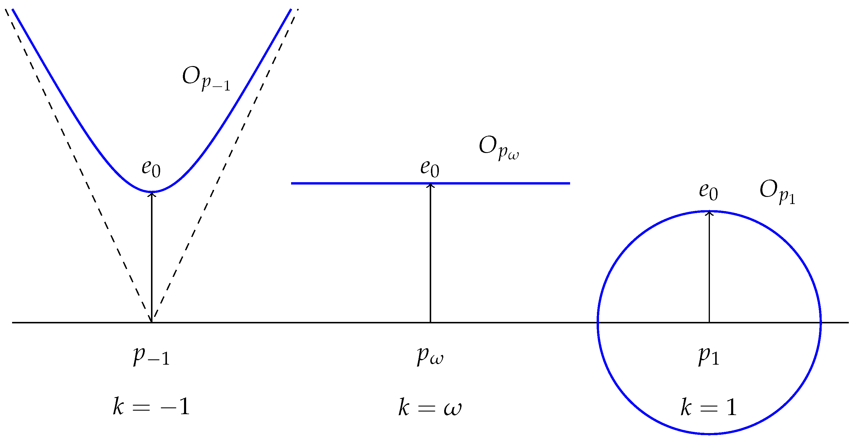
For convenience, let us introduce a new element by taking the most important information from S .
Definition 4.
The space of observers is the subset O of T M containing the first vector of each basis at S , and the space of observers at pis O p : = O T p M .
(i) 
In the region k > 0 , O contains all the unit vectors for g and each O p is a sphere.
(ii) 
In the region k <; 0 , O contains all the future-directed time-like unit vectors for g and each O p is a hyperboloid.
(iii) 
In the region k = , O is equal to Ω 1 ( 1 ) and each O p is an affine hyperplane not containing 0.
(iv) 
In the region k = 0 , O is equal to the absolute rest vector field W (so, each O p is a subset containing a single nonzero tangent vector).
Remark 3.
If n = dim M, then dim L M = n ( n + 1 ) and S L M is always a submanifold with dim S = ( n + 1 ) n / 2 . Nevertheless, O must be regarded as a subset of T M . Then, it becomes a smooth manifold of dimension 2 n 1 in the region k 0 but it collapses to a submanifold of dimension n when k = 0 .
The transition from Lorentzian to Riemannian through a region with k = ω can be easily understood by looking at O (see Figure 1). We will not be interested in the transition through a region with k = 0 . However, this could be described in a completely analogous way by defining a dual space of observers (constructed by picking at each point p the first element of the elements in the bases which are dual to those in S p ).

3.3. Pointwise Variation of Speed of Light

In the region < k < 0 , the function c ( p ) = | k ( p ) | might be understood as a variation of the speed of light with the point at M. Such a possibility has been speculated since the beginning of general relativity and was put forward in the 90s in relation to cosmological inflation and the horizon problem (see for example Reference [38,39,40,41] as well as some criticism in References [42,43]). In order to avoid the circularity of using the light to define the units to measure its speed, Barrow and Magueijo [44] argue that only the variation of adimensional constants would have a true physical meaning; so, the variation of c should be regarded as a variation of the (adimensional) fine structure constant α = e 2 / c 4 π ϵ 0 .
Without deepening into these questions, some comments about varying c in our framework are in order. Recall first that, in the affine case obtained by assuming Postulate 1, to assume also Postulate 2 would imply that all the IFRs would be using the same units for measurement and, then, the specific value of c would depend of the chosen units. Indeed, the natural interpretation of the group O ( k ) ( 4 , R ) for k = c 2 ( , 0 ) is just the Lorentz group in some appropriate coordinates. Thus, if one regarded the affine space Aff as a manifold and took different units at each point, then this could not be interpreted as a variable speed of light.
To measure a varying speed of light would rely on the possibility to compare the units of measurement at different points. In the affine case, such a comparison would be possible if the interactions were invariant by translations (an unlikely possibility). In general, one would need measurements involving magnitudes which are dimensionally independent (in particular, this would be achieved by measuring adimensional constants, as commented above). In principle, this might be achieved by measuring essentially different interactions, as in the case of light and gravity propagation (see below Definition 3)13. Anyway, as we will see, the Lorentz–Finsler viewpoint will open other possibilities by using infinitesimal anisotropy.

3.4. Relativistic vs. Leibnizian Structures

A priori, the cases < k < 0 and k = ω (with constant k and then c) are the physically interesting ones, either as a model of spacetime or as an approximation to this model. Next, they will be briefly compared.
In the first case, we will assume k = 1 on all M, after our discussion in the previous subsection. Therefore, one has a time-oriented Lorentzian metric g and O is a fibered space on M with fiber the hyperbolic space. Moreover, the Levi–Civita connection g is canonically associated with g, and any other affine connection ∇ parallelizing g (i.e., satisfying μ g ν ρ = 0 ) must be nonsymmetric. This selects g and provides a sense of free fall and light-like geodesics (compare with EPS later).
In the case k = ω , the Leibnizian structure consisting in the absolute time form Ω and the absolute space (ker ( Ω ) , h ) on M described in Section 3.1 is obtained. These structures were studied systematically in References [31,32]. In this setting, one considers Galilean connections, that is, affine connections ∇ which parallelize both Ω and h. It is worth pointing out that the set of all the Galilean connections has the same degrees of freedom as the set of all affine connections (symmetric or not) parallelizing a Lorentzian metric g. However, a symmetric Galilean connection will exist if and only if Ω is closed ( d Ω = 0 ), that is, locally Ω = d t for some function t . Nevertheless, in this case, there is no univocally determined symmetric connection. Moreover, this happens even if Ω is exact; that is, Ω = d t for some function t defined globally on M, which will be called the absolute time ( t is unique up to an additive constant). Indeed, an explicit Koszul-type formula reconstructs all the symmetric Galilean connections in terms of two data14 and Reference [31] Cor. 28, namely, the gravitational field (a vector field in the absolute space, that is, a section of the bundle ker ( Ω ) M ) and the vorticity (a skew symmetric 2-form on the vector bundle ker ( Ω ) ).
In conclusion, relativistic spacetimes are preferred to Leibnizian ones from the viewpoint of foundations because of two celebrated properties: (a) they permit to model a finite speed of propagation in vacuum (recall that observers appear now at each event as infinitesimal approximations to IFRs and, so, the arguments in Remark 2 apply), and (b) they select a unique affine connection in the set of all the connections parallelizing the geometric structure, while Leibnizian ones require the gravitational and vorticity fields as an extra input.
In the next section, we will focus only on relativistic spacetimes and the Finslerian extensions. Nevertheless, some previous elements serve as a background for the Lorentz and Lorentz–Finsler cases and they can be compared a posteriori with them (see Table 1). We point out a pair of them so that the interested reader might come back here later:
(1) Leibnizian structure ( Ω , h ) vs cone triple ( Ω , T , F ) (which is useful to define and to handle any cone structure C , Lorentz or Lorentz–Finsler; see Definition 8 and Remark 6(2)). Notice that, when F comes from a Riemannian metric h, then the Leibnizian structure can be regarded as a sort of limit when λ of the triples ( λ Ω , T / λ , F ) , which “open” the cone C .
(2) Chronometric vs EPS approach to spacetime (Section 5). The Leibnizian structure ( Ω , h ) (eventually, with Ω = d t ) gives a chronometric approach to spacetime in a similar way as the Lorentz metric does in relativitiy. However, the former requires an additional input (an affine connection) in order to define free fall. Therefore, the EPS approach (at least the axioms which do not consider light propagation) might also be interesting in the Leibnizian case. In contrast, the Lorentz–Finsler metric L will provide time-like and light-like geodesics in a very similar way as the Lorentz metric g in spite of the differences between the Levi–Civita g and the anisotropic connection (see Footnote 21) determined by L.
Note 1.
Newton–Leibniz controversy. To end this section, it is worth pointing out that the notion of Leibnizian structure provides a precise mathematical description of a historical controversy between Leibniz and Newton. Roughly speaking, Leibniz criticized Newton’s arguments about IFRs by pointing out that the Euclidean space perceived by an observer is equal even after a rotation of the observer’s coordinates. Therefore, he claimed that one could not detect whether these axes are being rotated at different times. Newton replied that spinning water in a bucket would detect whether the observer is rotating. From the mathematical viewpoint, Newton was using the structure of a Galilei–Newton spacetime, as described in Section 2.3 (that is, the linear quadratic classical space + time approximation in Table 1). Therefore, the overall affine structure of the (four dimensional) spacetime yields a natural affine connection, which can be used to detect rotation. Leibniz, however, is considering physical spacetime only as a manifold endowed with a Leibnizian structure (that is, he drops the spacetime affine structure and considers only the pointwise quadratic first nonlinear space + time in Table 1). Therefore, with these elements, no affine connection is determined and rotation cannot be measured. Summing up, Leibniz was right to point out that, only with the Leibnizian structure on M at hand, no Galilean connection is selected15. However, Newton did select such a connection by guessing the further affine structure of M.

4. Second Non-Linearization

4.1. Background: Norms, Cones, and Lorentz–Finsler Metrics

In order to show rigorously the emergence of the notion of Finsler spacetime, some purely geometric elements are stressed first. Even though some of them are elementary, they will be necessary to make precise discussions. Therefore, the experimented reader can skip some parts and come back when necessary.
The first ones come from classical norms on a (finite-dimensional, real) n-vector space V and Finsler Geometry; they are carefully explained in Reference [46].
Definition 5.
A Minkowski norm on V is a map F 0 : V R satisfying
(i) 
positiveness: F 0 ( v ) 0 , with equality if and only if v = 0 ,
(ii) 
positive homogeneity: F 0 ( λ v ) = λ F 0 ( v ) for all λ > 0 ,
(iii) 
strongly convex indicatrix: F 0 is smooth away from 0, and the fundamental tensor field g defined as the Hessian of 1 2 F 0 2 is positive definite on V \ { 0 } .
Remark 4.
Notice the following about this definition:
(1) 
Positive homogeneity. This requirement only for λ > 0 enhances the applications of Finsler Geometry16, and it will be enough for our purposes. Positive homogeneity implies that F 0 is univocallly determined by its indicatrix (unit sphere) Σ 0 : = F 1 ( 1 ) . In particular, the full homogeneity of F 0 becomes equivalent to the symmetry of Σ 0 with respect to the origin.
(2) 
Smoothness. The standard definition of norm implies that they are only continuous. We assume smoothness (say, C , pointing out the cases when lower regularity becomes relevant) away from 0. Using (ii), this is clearly equivalent to the smoothness of Σ 0 .
(3) 
Role of triangle inequality. It is not imposed directly, however,
(a) 
Triangle inequality becomes equivalent (for any 1-homogeneous function smooth away from 0) to the convexity of Σ 0 (i.e., its inner-pointing second fundamental form σ is positive semidefinite). Moreover, it is also equivalent to the convexity of the open unit ball B 0 : = F 0 1 ( [ 0 , 1 ) ) (all the segments connecting points u , v B 0 are included in B 0 ).
(b) 
The strict triangle inequality becomes equivalent to the strict convexity of Σ 0 (the hyperplane tangent to Σ 0 at each point p only intersects Σ 0 at p). Moreover, it is also equivalent to the strict convexity of the closed unit ball B ¯ 0 (segments connecting points u , v B ¯ 0 are included in the open ball B 0 up to the endpoints u , v ).
(c) 
Assuming (i) and (ii), hypothesis (iii) becomes equivalent to the strong convexity of Σ (σ is positive definite), which is more restrictive than its strict convexity.
(4) 
Conic Minkowski norms. These norms are as in Definition 5 just by allowing the map F 0 to be defined only on a cone domain (see Definition 7 below) A 0 of V. All the previous considerations on the triangle inequality extend trivially to such conic Minkowski norms.
(5) 
Scalar products. Norms coming from (Euclidean) scalar products are Minkowski. Conversely, a Minkowski norm comes from a scalar product under one (and then both) of the following properties:
(a) 
The classical parallelogram identity holds.
(b) 
F 0 2 is C 2 -smooth at zero [48] (Proposition 4.1).
Recall also that, clearly, any norm coming from a (Euclidean or Lorentzian) scalar product is determined by its value on a cone domain.
Definition 6.
A Finsler metric F on a manifold M is a function F : T M R satisfiying the following: (i) F is smooth away from the zero section 0 T M , and (ii) the restriction F p of F to each tangent space T p M , p M , is a Minkowski norm.
Remark 5.
Notice the following about this definition:
(1) 
2-homogeneity. Taking F 2 instead of F, Finsler metrics can be defined alternatively as positive 2-homogeneous functions (this will be convenient for their Lorentzian extensions). Furthermore, the C 2 -smoothability of F 2 at 0 would imply that it comes from a Riemannian metric (recall Remark 4 (5)).
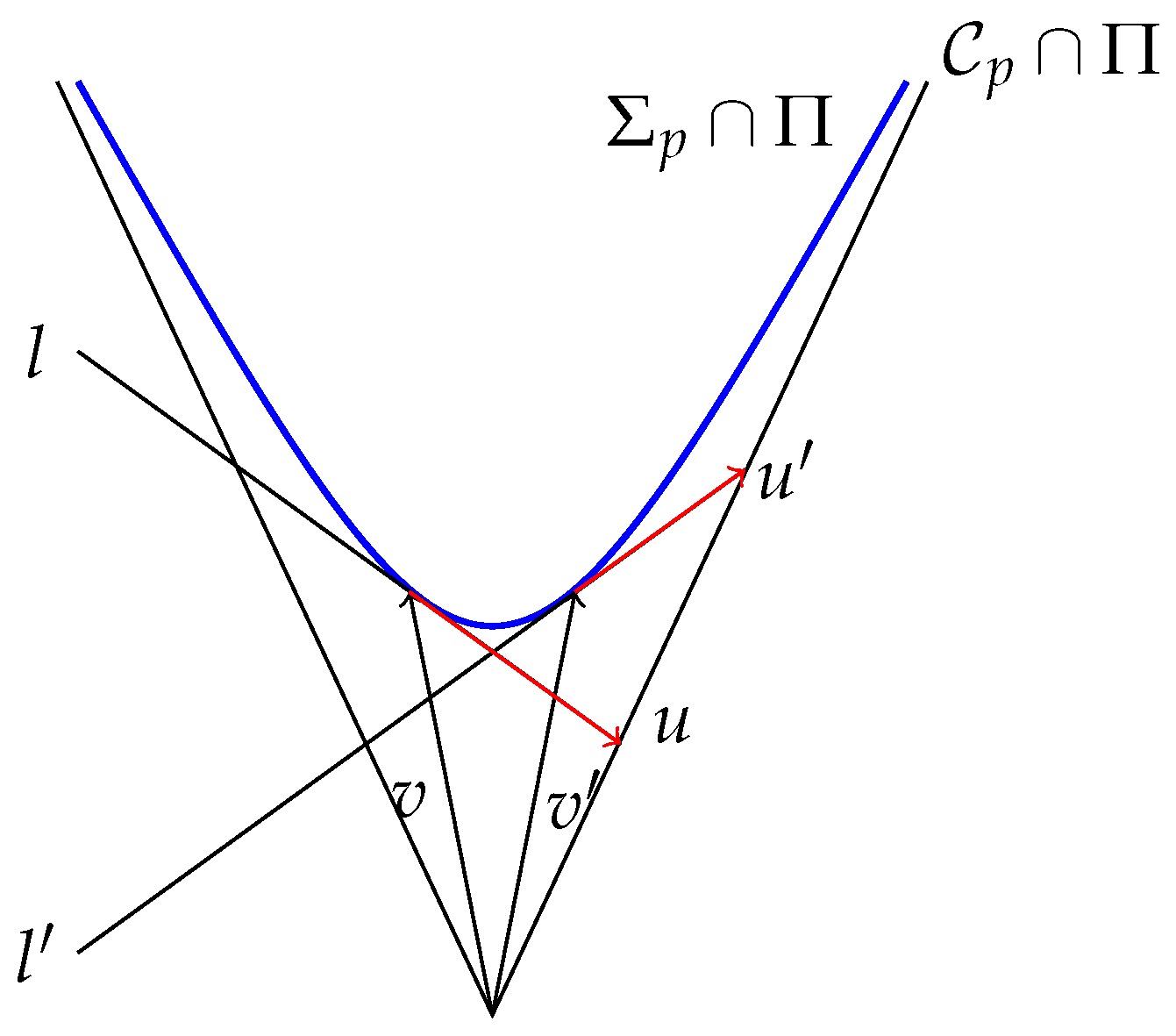
(2) 
Role of the indicatrix. As F is determined by its indicatrix F 1 ( 1 ) , a Finsler metric can be defined alternatively as a smooth hypersurface Σ embedded in T M satisfying appropriate conditions, namely, (a) Σ intersects transversely17 each T p M and (b) this intersection Σ p : = Σ T p M is a strongly convex compact connected embedded hypersurface whose inner domain B p (such that Σ p = B p , where ∂ denotes the boundary in V)18 contains the zero vector 0 p .
(3) 
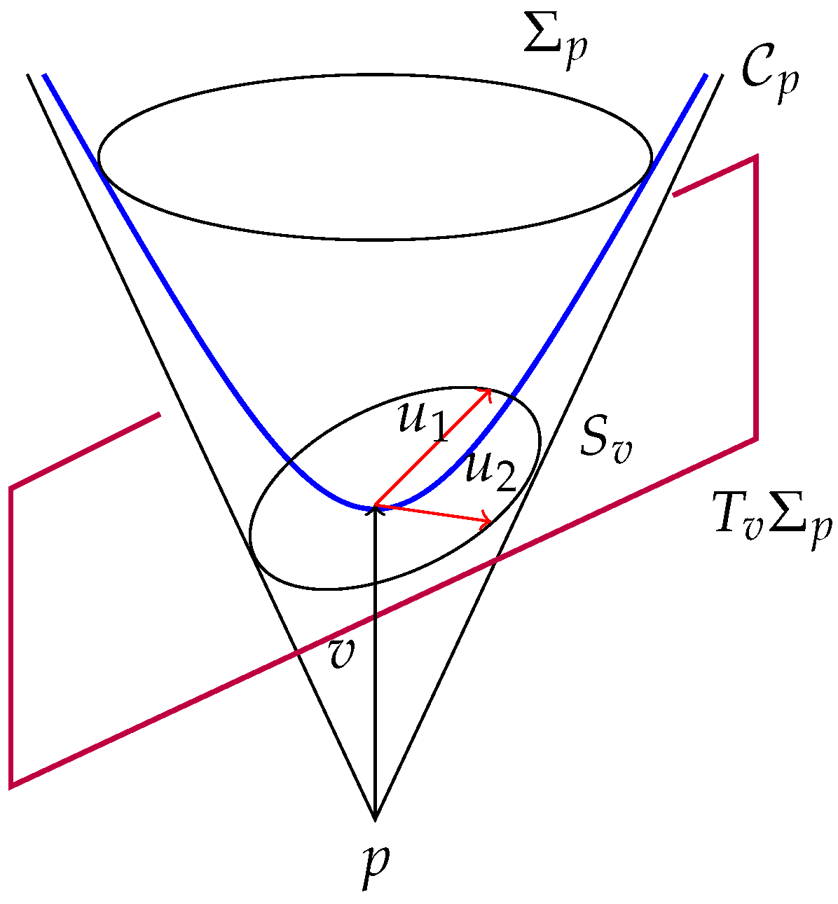
Fundamental tensor on a vector bundle. Each F p defines a fundamental tensor field on T p M \ { 0 } and, so, a 2-covariant tensor on each fiber of the (slit) tangent bundle π : T M \ 0 M . We will use the letter g to denote such a tensor field, so that, for each v T M \ 0 , g v will be a tensor on T p M , being p = π ( v ) . Clearly, the definition of Finsler metric and fundamental tensor can be extended to any vector bundle, not necessarily the tangent one.
The rest of elements involves the Lorentz–Finsler case, and we follow Reference [9]. We start with the definition of cone. For our purposes, the next one is enough. A more intrinsic definition can be seen in Reference [10] Def. 2.1 (the equivalence and related optimal assumptions are analyzed in Reference [10]) and Section 2.1.
Definition 7.
A (strong) cone C 0 in V is any embedded hypersurface which can be constructed as follows: choose a hyperplane Π V which does not contain 0 and a strongly convex compact connected embedded ( n 2 ) -hypersurface S 0 Π , take all the half-lines from 0 to the points of S 0 , and define C 0 as the union of all these half-lines except 0.
Then, the cone domain is the open subset A 0 obtained analogously by taking the (open) half-lines from 0 to each point of the inner domain B 0 of S 0 in Π (so that the boundary of A 0 in V \ { 0 } is C 0 ).
Definition 8.
A cone structure on a manifold M is a smooth embedded hypersurface C T M such that (a) C intersects transversely each T p M and (b) this intersection C p : = Σ T p M is a cone on T p M . Then, the cone (structure) domain is A = p M A p , where each A p is the cone domain of C p . A vector v A (resp. v C ; v A C ) is called time-like (resp. light-like; causal).
Remark 6.
Notice the following about this definition:
(1) 
Smoothness and transversality. Intuitively, a cone structure is just to smoothly put a cone at each T p M , p M . From the formal viewpoint, however, this cannot be deduced only from the smoothness of C , making necessary assumption (a) (recall Remark 5 (2) and footnote 17 or the discussion around Reference [49] Figure 2).
(2) 
Cone triples. Any cone structure C can be determined (in a highly nonunique way) by means of a cone triple ( Ω , T , F ) , where Ω is any time-like 1-form on M (i.e., Ω ( v ) > 0 for all causal v), T is any time-like vector field with Ω ( T ) 1 and F is the unique Finsler metric on ker ( Ω ) such that F ( w ) T + w C for any w ker ( Ω ) \ 0 [10] (Section 2.4). Conversely, any ( Ω , T , F ) with Ω ( T ) 1 and F Finsler on ker ( Ω ) is the cone triple of some cone structure C .
(3) 
Extended classical Causality. C allows one to extend basic elements of causality of spacetimes such as the chronological ≪, strict causal <, causal ≤, and horismotic → relations ( p q when p < q and p q ) and, thus, the chronological/causal futures and pasts of a point, I + ( p ) , I ( p ) / J + ( p ) , J ( p ) . In particular, cone geodesics are defined as locally horismotic curves and they generalize the future-directed lightlike pregeodesics associated with the conformal structure of any Lorentz metric.
In the following, we will say that a function is smooth in a manifold with boundary (contained in a regular manifold M) if it can be (locally) extended to a smooth function on an open subset of M.
Definition 9.
Let C 0 be a cone on V and A ¯ 0 = C 0 A 0 . A (properly) Lorentz–Minkowski norm with cone C 0 is a smooth map L 0 : A ¯ 0 R satisfying
(i) 
L 0 ( v ) 0 with equality if and only if v C 0 .
(ii) 
L 0 is positive 2-homogeneous: L 0 ( λ v ) = λ 2 v for all v A ¯ 0 and λ > 0 .
(iii) 
The fundamental tensor g obtained as the Hessian of 1 2 L 0 has Lorentzian signature ( + , , , ) on A 0 .
Remark 7.
Consistently with the positive definite case, let us observe the following:
(1) 
A less redundant definition for L 0 (as well as for the Lorentz–Finsler metric L below) can be carried out without prescribing the cone C 0 ; see Reference [10] Def. 3.1 and 3.5.
(2) 
Two homogeneities for L 0 are preferred to 1-homogeneity because of the general equality L 0 ( v ) = g v ( v , v ) . Notice also that the Lorentzian signature is changed with respect to previous sections, and consistently, if L 0 is smoothly extended around any v C 0 , then L 0 must become negative away from A ¯ 0 .
(3) 
L 0 is determined by its indicatrix Σ 0 = L 0 1 ( 1 ) , which is now strongly concave and asymptotic to C 0 . Indeed, a Lorentz–Finsler metric could be defined alternatively as a strongly concave hypersurface Σ 0 in A 0 which is asymptotic to some cone structure C 0 under the mild technical condition that the map A 0 v L 0 ( v ) such that v / L 0 ( v ) Σ 0 extends smoothly to C 0 with nondegenerate19g.
(4) 
All the properties related to the triangle inequality in the positive definite case (which were associated with the convexity of the indicatrix and held for conic Minkowski norms; Remark 4 (3) is automatically translated now as reverse triangle inequalities in the Lorentz–Finsler case (associated with the concaveness of Σ 0 ).
(5) 
Even though A ¯ 0 V \ { 0 } , L 0 can be continuously extended to 0 ( L 0 ( 0 ) = 0 ). However, the smoothness of this extension20 depends on whether L 0 comes from a Lorentzian scalar product, as in the positive definite case.
(6) 
It is possible to smoothly extend L (preserving the 2-homogeneity) to an open conic subset A 0 * which contains A ¯ 0 (recall that 0 A ¯ 0 ). This extension is far from unique, but the fundamental tensor in the boundary is well determined.
Definition 10.
Let C be a cone structure on M and A ¯ = C A . A (properly) Lorentz–Finsler metric with cone C is a smooth map L : A ¯ R satisfying that the restriction L p of L to each T p M A ¯ is a Lorentz–Minkowski norm. Then, ( M , L ) is A (properly) Finsler spacetime.
Remark 8.
The following results on Finsler spacetimes will be relevant:
(1) 
Any Lorentz–Finsler metric can be extended to T M \ 0 as a smooth 2-homogeneous function with fundamental tensor g of Lorentzian signature; see [12]. However, such an extension is highly nonunique and, as we will see, it is not justified by direct measures of observers.
(2) 
Given L, time-like and light-like geodesics are naturally defined, and they satisfy local maximizing properties which extend those of relativistic spacetimes (recall Remark 7(4) and Reference [10] Prop. 6.5). In particular, the light-like pregeodesics of L coincide with the cone geodesics of C [10] (Section 6.2).
(3) 
Thus, all the Lorentz–Finsler metrics with the same cone structure have the same light-like pregeodesics. Two such metrics, L 1 and L 2 , are called anisotropically equivalent, and they satisfy L 2 = μ L 1 for some 0-homogeneous function μ > 0 on A ¯ [10] (Section 3.3).
(4) 
Any cone structure C is associated with a Lorentz–Finsler metric L (and, then, with its anisotropically equivalent class). Indeed, if C is determined by a cone triple ( Ω , T , F ) , one can construct such an L starting at the map
G ( v ) : = Ω ( v ) 2 F ( π 2 ( v ) ) 2 , v A ¯ ,
where π 2 : T M = Span ( T ) ker ( Ω ) ker ( Ω ) is the natural projection. G satisfies all the required properties of L except the differentiability on Span ( T ) , the latter because of the lack of differentiability of F 2 at 0 when it is not Riemannian. Indeed, the indicatrix G 1 ( 1 ) A is not smooth precisely on T, that is, only at the point T p on each p. However, standard techniques of smoothability for convex functions allow one to smoothen G around T obtaining the required L [10] (Section 5.2).
(5) 
The lack of differentiability of G above is analogous to the well-known lack of differentibility of any product of (non-Riemannian) Finsler manifolds. Indeed, if ( M 1 , F 1 ) is a Finsler manifold, then d t 2 ( ± F 1 2 ) is not smooth as Finsler or Lorentz–Finsler metrics on R × M 1 along the direction t . This problem prevents the extension to the Lorentz–Finsler case of the trivial procedure to construct a relativistic product spacetime starting at a Riemannian manifold.
(6) 
Given a Lorentz–Finsler metric, there exists a univocally determined A-anisotropic connection which is torsion-free and parallel. Moreover, when we consider a properly Lorentz–Finsler metric, this A-anisotropic connection can be extended to an open subset A * which contains A ¯ \ 0 . As the extension away from A ¯ is highly nonunique, we will speak about A ¯ -anisotropic connections. When A = T M \ 0 , we will just say anisotropic connection21.
Due to this last item, the definitions of some classes of Finsler spacetimes such as the static ones have included the possibility to have some non-smooth directions [2,3,54]. However, the smoothing procedure mentioned in part (4) of Remark 8 is also applicable to these cases. This shows that, from the foundations viewpoint, the motivation for non-smooth metrics is not stronger for the Lorentz–Finsler case than for classical relativistic spacetimes [10] (Sections 4.2 and 4.4).
Note 2.
Nevertheless, there are some physical considerations (see Section 6.1) which lead to examples where L is not smoothly extendible to the cone structure C , even if
(i) its cone C is smooth (so, the cone geodesics are well defined), and
(ii) the A-anisotropic connection can be smoothly extended to C (so, the Finslerian curvature tensors are well defined on C ).
Such examples could also be included in our definition of Lorentz–Finsler metrics and spacetimes, as all the relevant geometric properties remain. However, we will consider for simplicity that L is smooth at C and, when this property does not hold, we refer to them as improper and we will discuss whether (i) and (ii) hold then. Accordingly (and consistently with Reference [10] Def. 3.1), an improper Lorentz–Minkowski norm L 0 satisfies all the properties in Definition 9 but the differentiablility at L 0 1 ( 0 ) .
Remarkably, a large class of spacetimes satisfying both conditions (i) and (ii) can be found following Reference [22]. Namely, they hold for any two-homogeneous function L defined on the set of causal vectors A ¯ determined by a cone structure C such that (a) L is zero on C and determines a Lorentz–Finsler metric in the interior A of A ¯ and (b) there is a power of L which is smooth on C with nondegenerate Hessian (notice that, in Reference [22], L is assumed to be defined on the whole T M ).
Anyway, there are some examples of Finsler spacetimes in the literature that do not even satisfy our weaker definition of improper Lorentz–Finsler spacetime, such as Randers spacetimes or those introduced by Kostelecky [55,56], which are the effective model of some particles with no GR background (see the discussion in Reference [10] and Appendices A and B).

4.2. Physical Intuitions for Finsler Spacetimes

Next, our aim is to justify physically our definition of Finsler spacetime (Definition 10), supported by some mathematical properties pointed out above. The first consideration is that Postulate 2 should be regarded now as an approximate symmetry at each point in a similar way as the affine structure of Postulate 1 has been regarded as an approximate symmetry to the structure of a relativistic spacetime22. This means that, now, one cannot find a set of coordinate charts such that the relations in Equation (3) occur at each p; however, one would expect that we will not be far from this situation (at least in regions of spacetime free of extremely exotic or violent situations). Consistently, we will not have the sets S p of linear bases at each T p M playing the role of (linear) IFR at p. However, one would expect that the set of observers O introduced in Definition 4 will still make sense and will be “close” to the space of observers for a relativistic spacetime. As the latter is a hyperboloid (asymptotic to a quadratic cone) at each point p, now, O p should be a strongly concave hypersurface asymptotic to some cone structure defining a Lorentz–Minkowski norm at p (see Remark 7 (3)), and moreover, O should be identified as the indicatrix Σ of a Lorentz–Finsler metric L.
Remark 9.
The previous discussion leads us to a Lorentz–Finsler metric L with indicatrix Σ equal to O which lies exactly under our Definition 10 (including also the improper case explained in Note 2). The way to arrive at this definition from the viewpoint of symmetries can be summarized as follows.
(1) Following [23], consider the connected parts of the identity I S O 1 ( 4 ) , S O 1 ( 4 ) , I S O ( 3 ) , and S O ( 3 ) of the Poincaré, Lorentz, Euclidean, and orthogonal groups, resp. In special relativity, the homogeneous spaces obtained as the quotients I S O 1 ( 4 ) / S O 1 ( 4 ) , I S O 1 ( 4 ) / I S O ( 3 ) , and I S O 1 ( 4 ) / S O ( 3 ) are, respectively, the spacetime, the space of all the (rest) spaces (i.e., the space of all the spacelike hyperplanes, being the standard rest space I S O ( 3 ) / S O ( 3 ) ), and the space of observers O (being the space of velocities S O 1 ( 4 ) / S O ( 3 ) ). Here, O is metrically identifiable with R 4 × H + 3 .
(2) In general relativity, O is identified with the set Σ g of all the future-directed unit vectors. Σ g is a subbundle of T M in which the fibers are affine hyperboloids at each tangent space. Such hyperboloids characterize g univocally so that the information of g is codified in O .
(3) For the space of observers O in the Lorentz–Finsler setting, Σ g is replaced with a hypersurface Σ satisfying formal properties analogous to Σ g (but dropping its pointwise symmetries) so that it characterizes a Lorentz–Finsler metric.
Next, let us discuss more carefully the physical grounds of Definition 6:
(1)
The fact that L is defined only on a cone domain A and that it is extended continuously to C comes from the nature of the space of observers.
Recall that, then, one has time-like geodesics (Remark 8 (2)) and, thus, freely falling observers. At least from a trivial mathematical viewpoint, this is enough to determine L and, then, the fundamental tensor g on the cone domain A.
Notice that, given an observer v Σ p , the tensor g v is then also obtained on the directions of T v Σ p . In principle, g v (which can be obtained just from Σ ) could be measured, as it comprises properties of neighboring observers.
(2)
The smooth extensibility of both L and the fundamental tensor g (as a nondegenerate one) to the cone structure C appears as a natural approximation (in principle, one would expect to remain close to the situation in a relativistic spacetime) which mathematically ensures that C is truly a cone (with S 0 in Definition 7 satisfying strong convexity). Moreover, then L also determines light-like geodesics which, up to reparametrization, are inherent to the cone structure. The improper case of Finsler spacetimes satisfying the properties (i) and (ii) in Note 2 would also satisfy all these properties about geodesics and cones.
Then, as a consequence, the behaviour of lightlike geodesics becomes completely analogous to the classical relativistic case. Indeed, Lorentz–Finsler metrics with the same cone structure are also related by an “anisotropic conformal factor μ ” (Remark 8(3)) and the cone structure C also allows one to mimic the relativistic behaviour of causality (Remark 6(3)).
(3)
The physical considerations in the two previous items are also assumed in standard relativity. Namely, observers are always expected to measure only massive or massless particles, that is, elements with velocities in a causal cone. In seneral relativity, this is apparent from the EPS formulation, where radar coordinates are systematically used with this aim (see the next section). Certainly, the metric tensor g is assumed to be defined on all the directions in the relativistic case but the underlying reason is that g is fully determined by its value along the causal vectors (Remark 4(5)). This is not by any means true in the Lorentz–Finsler case, even if L can be extended to the whole T M (recall Remark 8(1)).
(4)
When a space-like separation in a direction l is going to be measured by an observer v, it seems natural to consider g v ( l , l ) ; therefore, it would be irrelevant whether L is not defined outside the cone.
Indeed, from a purely geometric viewpoint, T v Σ p would be naturally regarded as the rest space of the observer v at p and that g v would be the unique metric available there, even though the physical process to measure it might not be obvious. It is worth pointing out here Ishikawa’s claim in Reference [8] that g v ( l , l ) can be measured, assuming that the physical light rays are those of g v . Indeed, this author criticizes Beem’s definition of light rays, which was constructed by using the light-like vectors on the cone C . Anyway, in our opinion, Ishikawa’s claim needs further physical support.
(5)
It is worth emphasizing that no issue on smoothability occurs with Σ , which can be assumed smooth (as in Remark 4(2)) in most interesting cases.
(a) The Lorentz–Finsler metric L cannot be C 2 -extended to 0 in agreement with the behavior of norms in both the positive definite case and the Lorentz–Finsler one (Remark 4(5)). However, no physical or mathematical reason seems to require the smoothability of L at 0 (compare with the EPS approach in Section 5.2.1 below).
(b) Product metrics d t 2 + F 2 or, with more generality, the rough Lorentz–Finsler version of static spacetimes Λ ( x ) d t 2 + F 2 ( x , y ) , with natural coordinates ( x , y ) at T M are never smooth at t whenever F is Finsler but not Riemannian. Consequently, some authors have included the possible existence of non-smooth directions as a fundamental ingredient of Lorentz–Finsler metrics (see for example References [2,3,54]). Nevertheless, as explained in Remark 8, parts (4) and (5), general smoothing procedures can be applied. Furthermore, a natural definition of (smooth) static spacetimes as well as an explicit procedure to construct locally all of them are available in Reference [10] (Section 4.2).
(c) Other issues of non-smoothness appear when modelling some specific physical situations (very special relativity and birefringence) and will be considered in Section 6.1.

5. Comparison with Ehlers–Pirani–Schild Approach

5.1. Summary of the Approach

EPS approach [19] constructs step by step each geometric structure of physical spacetime (until reaching the metric) by means of physically motivated axioms:
(1)
Spacetime becomes a differential manifold M endowed with a cone structure C . Essentially, this is obtained by means of axioms on light propagation which involve messages and echoes between particles.
Indeed, these axioms allow one to find radar coordinates with respect to (freely falling, massive) particles, the latter represented by a class of unparametrized curves, which provide the structure of differentiable manifold, see EPS axioms D 1 D 4 . Then, the cone structure C is obtained by using two axioms, L 1 , L 2 , on the local character of light propagation around each event e. Indeed, L 1 states that, given any particle P with some parameter t which passes through e, it follows that any event p ( p P) can be connected with the particle by exactly two light rays23, while L 2 distinguishes two connected components for light rays. Moreover, L 1 also states that, if these two rays cross the curve at the events e 1 , e 2 , then g ( p ) : = t ( e 1 ) t ( e 2 ) is required to be smooth in a small neighborhood of e. EPS claims that, then, C will come from the conformal structure of some Lorentz metric (a particular case of our Definition 8) and, so, we can speak about C -time-like directions.
(2)
Spacetime is endowed with a projective structure P . This is achieved by means of two axioms, P 1 and P 2 , which model the free fall of particles.
The first one states only the existence of a unique particle, represented by means of an (unparametrized) curve, for each event e and C -time-like direction at e. The second axiom states that, around each event e, one can find coordinates x ¯ i such that any particle through e admits a parametrization x ¯ ( u ¯ ) satisfying
d 2 x ¯ i d u ¯ 2 e = 0 .
This equality is regarded as an infinitesimal law of inertiA (consistently with Trautman [57]). By using Equation (10), EPS argues that a projective structure, which is claimed to be compatible with some affine connection A , must appear. As a consequence, not only the original particles would be recovered as pregeodesics of A but also one would obtain pregeodesics at any direction, time-like or not.
(3)
Spacetime is a Weyl space ( M , C , A ) , where A is an affine connection compatible with the cone structure C , in the sense that the light-like C -pregeodesics are also A -pregeodesics. This is carried out by means of their axiom C, which matches particles and light rays.
Specifically, this axiom assumes that, around each event e, any point in the C -chronological future of e lies on a particle through e. This will imply that the light-like C -pregeodesics of the conformal structure (namely, the C -cone geodesics; see Remark 8(2)) are also pregeodesics for the projective structure P in step (2). Then, EPS claims that such a compatibility selects a unique affine connection A compatible with the projective structure.
(4)
Spacetime is endowed with a (time-oriented) Lorentzian metric g, up to an overall (constant) scalar factor. This is obtained by means of a Riemannian axiom, which takes into acccount that A has its own parallel transport and its curvature tensor; the axiom imposes the compatibility of (one of) these two elements with g.
Indeed, they state that the Riemannian compatibility of ( M , C , A ) is equivalent to any of the following conditions: (a) the vectors obtained by A -parallel transport of a single one v at p M along two curves with the same endpoint q have the same norm at q (computed with any of the homothetic scalar products compatible with C q ), or (b) using Jacobi fields to construct arbitrarily close particles, the proper times of two of such particles are linearly related at first order, that is, the regular ticking of a clock for the first particle implies the regular ticking for the second one.
About these axioms and proofs, EPS admits: “a fully rigorous formalization has not yet been achieved”. Next, we will focus just on the relation of EPS approach with Lorentz–Finsler metrics. For progress on EPS approach, see for example Reference [58].

5.2. Keys of Compatibility with Finslerian Spacetimes

The fact that a Finslerian spacetime can fulfill the EPS axioms was already pointed out by Tavakol and Van den Berg [15], who considered the case of Berwald spaces. Now, our aim is to revisit precisely the compatibility of the four EPS steps with Finslerian elements [15].

5.2.1. EPS Step (1)

Recently, Lammërzhal and Perlick [11] have argued against the role of smoothness of the function g ( p ) at e in step (1). This differentiability becomes essential because the equalities g ( e ) = 0 , g , a ( e ) = 0 allow EPS to find a metric tensor g , a b ( e ) compatible with C .
Indeed, there are subtle differences at this point in comparison with the introduction of radar coordinates, which are used to settle the smooth ( C 3 ) manifold structure of the spacetime. Certainly, EPS were aware of the existence of nontrivial subtleties, as one can read at the beginning of their subsection Differential Topology: “The reason that we do not take this structure [smooth manifold] for granted is that differentiability plays a crucial role in our introduction of null cones (...) and in the infinitesimal version of the law of free fall”. The following three items must be taken into account in the EPS development:
(i) The axioms D 1 D 4 , which allow one to define radar coordinates, should apply to particles P and Q which do not intersect. Otherwise, spurious differential issues might appear even in the case of Lorentz–Minkowski spacetime24.
(ii) Axiom L 1 , however, considers the functions p t ( e 1 ) and p t ( e 2 ) (which would be radar coordinates for some particle P through e) defined even on P. Moreover, this axiom ensures that the particular combination g ( p ) = t ( e 1 ) t ( e 2 ) is C 2 -differentiable on P too.
(iii) In the discussion above [19] Lemma 1, they explain that t ( e 1 ) = t ( e 2 ) = 0 occurs if and only if p = e = e 1 = e 2 (thus, p P) and they focus on this case. Then, EPS argues first that the differential g , a ( e ) must be 0 by applying L 2 and, using C 2 differentiability, they show that the light directions must lie in the quadratic cone of the lightlike vectors of g , a b ( e ) .
Recall, however, that there is no physical justification about why g must be differentiable or C 2 . Notice that g is constructed from the functions e t ( e 1 ) and e t ( e 2 ) , which are not smooth even in the Lorentz–Minkowski spacetime (see Example 1 below). This assumption on the product t ( e 1 ) t ( e 2 ) yields a posteriori the quadratic character of the cone, forbidding more general cone structures.
From a purely mathematical viewpoint, the smoothness issue on the radar coordinates above would be similar to the differentiability of the radial coordinate r of a normed vector space at 0: r is never smooth at 0 and r 2 is smooth if and only if the norm comes from a Euclidean scalar product (Remark 4(5)). Therefore, such an a priori assumption would be completely unjustified from a mathematical viewpoint too:
(a)
There are norms with an analytic indicatrix (thus, analytic away from 0) which do not come from a scalar product. For example, on R 2 , when the indicatrix is equal to the curve in polar coordinates ρ ( θ ) = 1 + ϵ sin θ for small ϵ > 0 (so that it is strongly convex).
(b)
Euclidean scalar products are very particular cases of analytic norms.
That is, the apparently mild EPS requirement of differentiability at 0 becomes even stronger than analyticity for a norm.
Example 1.
Let us see the role of smoothability for the EPS function g obtained by using a pair of radar coordinates with respect to a particle (according to EPS, one should take two pairs of radar coordinates by choosing two particles). We will work on M = R × R 3 . Let t : R × R 3 R be the natural projection, consider any Minkowski norm F 0 on R 3 and take spherical-type coordinates ( r , θ , φ ) on R 3 (up to suitable points) with θ , φ , the usual spherical angles, and r F 0 ; then, extend the functions r , θ , φ to R × R 3 in a t-independent way. Let C be the natural (constant) cone structure given by t ( p ) = r ( p ) and regard the t-axis as a particle P. The corresponding radar coordinates are t ± r , and thus, the EPS g is g ( p ) = t 2 ( p ) + r 2 ( p ) . This function is smooth at 0 if and only if F 0 comes from a Euclidean scalar product25. Anyway, the cone structure is smooth because it is determined by the cone triple ( d t , t , F 0 ) and, so, it is compatible with a smooth Lorentz–Finsler metric L (indeed, a Lorentz–Minkowski norm); see Remark 8(4). As stressed in item (5) below Remark 9, the fact that d t 2 + F 0 2 is not smooth at t neither contradicts the existence of a smooth L nor introduces any issue of smoothability.

5.2.2. EPS Step (2)

The way EPS deduces the existence of the projective structure P from the infinitesimal law of inertia in Equation (10) consists in rewritting this last formula in arbitrary coordinates to obtain Reference [19] Equation (7)
x ¨ a + Π b c a x ˙ b x ˙ c = λ x ˙ a
where λ depends on the parameterization x a ( u ) of the curve and Π b c a depends on x a . These functions are called the projective coefficients, as they would determine a projective structure P compatible with some affine connection.
However, if one allowed the functions Π b c a to depend on the direction of the velocities x ˙ j , then Π b c a ( x i , x ˙ j ) could represent the formal Christoffel symbols for a Lorentz–Finsler metric L (indeed, for its A-anisotropic connection, see Remark 8, item 6). Thus, the solutions of Equation (11) would be pregeodesics for L which satisfy the law of inertia in Equation (10), up to the following issue of C 2 -differentiability of the chart coordinates at the origin.
The existence of normal coordinates in C -time-like directions (which is ensured for any A-anisotropic connection26) would be the natural mathematical translation for the law of inertia. However, the Christoffel symbols of a Lorentz–Finsler metric might not be even continuous at the origin by the trivial reason that these symbols may depend on the direction but they cannot vary along each direction (they are homogeneous of degree 0). Thus, its exponential map is not guaranteed to be C 2 at the origin unless the anisotropic connection is affine (i.e., it does not depend on the direction). It is known that, for a positive definite Finsler metric, this happens if and only if the metric is of Berwald type27 [60] (see also Reference [61] Ex. 5.3.5) and this can be extended to the Lorentz–Finsler case. Indeed, this type of metrics provides the Lorentz–Finsler examples beyond EPS suggested in the literature; see Section 5.2.5.
Summing up, we emphasize (a) that the coordinates provided by the exponential map of a Lorentz–Finsler metric at any event e are smooth along the half-lines starting at e and they satisfy Equation (10) and (b) excluding anisotropic connections because their lack of smoothness at 0 is a subtle mathematical issue and (as in the discussion of the step 1 in Section 5.2.1) this is not justified in EPS, neither physically nor mathematically. Thus, the law of inertia should be regarded as compatible with Lorentz–Finsler metrics according to our definition (where the directions outside the causal cone are not taken into account), including even the improper case in Note 2).

5.2.3. EPS Step (3)

The compatibility of ( C , P ) as a Weyl space with a (unique) affine connection A obtained by using EPS axiom C becomes a subtle question. On the one hand, Trautman [62] claimed the necessity of a detailed proofs in his review on the reprinted EPS article and, shortly after, this author and V. Matveev [63] characterized when a pair ( C , P ) is compatible. On the other hand, the notion of Weyl space as the triple ( M , C , A ) given by EPS does not coincide with the standard one of Weyl geometry28. Some authors questioned whether such an EPS structure permits to define a standard Weyl one as well as EPS development at this step. However, very recently, this question has been positively answered by Matveev and Scholtz [66], vindicating the EPS approach.
We emphasize that the EPS compatibility axiom C can be stated with no modification in the case that C is any cone structure and P is the projective class of pregeodesics of any A ¯ -anisotropic connection defined on all the C -causal directions (as already commented, C determines intrinsically cone geodesics extending those in EPS conformal cones (Remark 6(3))). Therefore, the possibility to extend previous results to this setting should be explored.

5.2.4. EPS Step (4)

In the EPS spirit, the Riemann axiom would be any (minimum, physically well-motivated) assumption making a compatible triple ( C , P , A ) also compatible with a Lorentzian metric, as the conditions labelled (a) and (b) at step (4). However, in order to state now a Finslerian axiom, one should notice that these conditions involve A and, so, they might depend on the way the previous step is solved.
Anyway, it is worth pointing out some reasons which would support the convenience of such a Finslerian axiom. On the mathematical side, the results collected in Remark 8 (parts (3) and (4)) show a natural consistency: (i) any C can be associated with a Lorentz–Finsler metric L, (ii) any other associated L is anisotropically related to L, and (iii) the light-like pregeodesics of all the associated Lorentz–Finsler metrics agree with the cone geodesics of C . On the physical side, the standard chronometric approach is reduced to the determination of the indicatrix of the observers at each event, and this would depend only on the behaviour of clocks and measurements of proper time29. Notice that, in the Finslerian case, this behaviour would not be restricted by any condition of quadratic compatibility (but only by a mild overall concaveness and asymptoticity to C ).

5.2.5. Finslerian Examples Strictly Compatible with EPS

As we have explained, the requirement of C 2 smoothability at 0 for cones and geodesics is the main gap in the EPS approach. However, Tavakol and van der Berg [15] showed Finslerian examples which are even compatible with this requirement. Next, let us analyze these and other possible examples of Finsler EPS compatible (FEPS) spacetimes.
A very simple FEPS example would be the following. Consider an affine space endowed with any Lorentz norm L 0 with the same cone as a Lorentzian scalar product · , · ( L 0 can be obtained by perturbing the indicatrix of · , · , as explained in Remark 8, item (4)). Then, the cone and geodesics of L 0 would satisfy all the EPS axioms, including those of C 2 smoothness at 0. Here, the key is that the affine parallel transport preserves both the indicatrix of L 0 and · , · .
Remark 10.
The Tavakol and van der Berg examples also obey this pattern, even though they are more refined and interesting. Indeed, they are Berwald-type spacetimes constructed by using an auxiliary Lorentz metric g. The fact that they are FEPS examples becomes apparent because they have the same cone and geodesics as g.
However, we emphasize that these FEPS examples are not in contradiction with the EPS conclusions. Indeed, the above examples only show that the physical elements C , A , under the EPS restrictions, may be compatible with two different geometric structures: the Lorentz g and Lorentz-Finsler L metrics. To decide which of them would be physically more appropriate would depend on further physical input. In absence of such input, the use of g would be mathematically simpler. Nevertheless, this input might appear from the measurements of proper time, as suggested at the end of Section 5.2.4.
In order to obtain a true Finslerian contradiction with EPS conclusions, one should construct a Lorentz–Finsler metric L with associated cone C and anisotropic connection A satisfying
(i) the EPS C 2 requirements,
(ii) the cone geodesics of C being pregeodesics of A ,
(iii) C being invariant under the A -parallel transport, and
(iv) A being not compatible with any Lorentz metric.
However, the following known results on linear algebra and Finsler metrics suggest the difficulty to find such a contradiction. Notice that the Finslerian results have been obtained in the positive definite case (the last one after the original EPS paper) and their suitable extensions to the Lorentz–Finsler case is not always clear:
(a) The square of a norm is C 2 at 0 if and only if it comes from an Euclidean scalar product ([48], Section 4.2, item 5 (b)). As a consequence, the C 2 requirement (i) implies the Lorentzian character of the cones (Section 5.2.1).
(b) A linear map between two Lorentzian vector spaces is homothetic if and only if it preserves the lightcones 30. As a consequence, if C is compatible with a Lorentzian metric g (as established in (a)), the preservation of C under A -transport in (iii) implies that this transport must be a g-homothety; in particular, the Riemann axiom (its version (a) in Section 5.1, item (4) is satisfied.
(c) The exponential of a Finsler metric is smooth at 0 if and only if it is Berwald [60]. As a consequence, the law of the inertia (with the C 2 requirement (i)) would imply that only Berwald-type Lorentz–Finsler metrics could be admitted (Section 5.2.2).
(d) All Finsler metrics of Berwald-type metric are affinely equivalent to a Riemann space; that is, their affine connections are Levi–Civita for Riemannian metrics (Szabó, [68]).
Notice that, in the case that a suitable Lorentz–Finsler version of this last result existed (taking into account, eventually, requirement (ii)), this would imply that FEPS is also compatible with a Lorentz metric; that is, the requirement (iv) could not be fulfilled if (i), (ii), and (iii) held.
Remark 11.
Recently, Fuster et al. [69] have shown that there are Berwald-type Finsler spacetimes which are not affinely equivalent to a Lorentz metric. However, they contain non-smooth directions; this must be taken into account for the comparison with Szabó’s result or the possible contradiction with EPS. Anyway, they show a minimal violation of smoothness. Indeed, their examples include improper Lorentz–Finsler metrics L, satisfying both (i) and (ii) in Note 2 and, moreover, they satisfy that some power L r (with r > 1 and integer) is smooth even at the light-like directions of their cone; see Remark 15.
Remark 12.
Recently, Hohmann et al. [70] have classified the Berwald spacetimes which are spatially homogeneous and isotropic. Among them, they have found a genuinely Finslerian class (with cones equal to classical FLWR spacetimes). As a proper Finslerian extension of relativistic cosmological spacetimes, the interest of this FEPS class is remarkable (even if it is not clear that they yield a true contradiction with EPS or not).

5.3. Constructive EPS Approach vs. Observer’s Approach

In order to compare EPS approach and ours, notice first that EPS distinguishes between a chronometric approach à la Synge [71,72] and their constructive approach. The former one regards the concepts of particle and standard clock as basic and introduces the metric g as fundamental. Therefore, it regards as primitive an easily measurable physical quantity (proper time) and a single geometric structure (the metric), the latter encoding all the other geometric elements in a simple way. As a consequence of these advantages, the chronometrical approach is very economical. However, EPS also pointed out drawbacks:
(1)
the impossibility to construct the metric from the behavior of the clocks alone,
(2)
the inclusion by hand of the hypothesis that metric geodesics will correspond with free motion, and then,
(3)
the expectation that the clocks constructed by means of freely falling particles and light rays will agree with the metric clocks.
This motivated their constructive approach starting at basic elements (events, particles, and light rays) and axioms close to the physical experience. Certainly, EPS aimed to deduce the metric structure from their axioms. However, the difficulties found in some points (as explained in Section 5.2.3, step (3) would have been solved only very recently) as well as the necessity to introduce a Riemannian axiom at the end makes the procedure somewhat awkward.
In contrast, our approach is neither chronometric nor constructive; instead, it only appeals to the way we measure. As such, a procedure is complex: one starts at the ideal situation when some symmetries among measurements are assumed (our two postulates). Under our viewpoint, if such symmetries did not hold at all, it would not be clear even the meaning of the verb “to measure”. However, in the case that the symmetries can be invoked as an approximation, the meaning of measurements can be recovered. Then, the emergence of some geometric structures resembles a sort of experimental Klein’s Erlangen program.
Notice that only hypotheses on the way of taking coordinates of space and time (inertial reference frames and observers) were assumed. It is noteworthy that only some few possibilities emerged for the geometry of spacetime when these symmetries hold in a strict way. From the standard physical viewpoint (close to philosophical realism), the fact that the space, time, and matter allow us to measure in some specific way should be interpreted as an evidence about the power of the emerged geometric structures in order to describe the physical spacetime.
Anyway, it is also worth noticing that our final geometric model of spacetime (a manifold endowed with a Lorentz–Finsler metric defined only on the set A ¯ of causal vectors for a cone structure) is compatible with EPS approach. Indeed, as shown in the previous subsection, EPS excluded the properly Finslerian case only due to two mathematical subtleties about unjustified restrictions of smoothness in radar coordinates (step (1)) and the law of inertia (step (1)). As pointed out in our discussion at Section 5.2.4, in the case that C (or the Weyl pair ( C , P ) in the step (4)) were not assumed to be compatible with a Lorentz metric, the Riemannian axiom might be replaced by a Finslerian one which would involve only the behaviour of clocks.
Finally, we emphasize that EPS approach also gives a strong support to our hypothesis that, in principle, the Lorentz–Finsler metric must be defined only at the causal directions in A ¯ : no basic element in the EPS approach (particle, light rays, radar coordinates, and echoes) involves noncausal directions.

6. Lorentz Symmetry Breaking

The implications of the introduction of Finslerian geometry may be more transparent if we focus on the Lorentz symmetry breaking, which occurs when Lorenz–Finsler norms are used to extend special relativity (i.e., when one considers only the second non-linearization in Table 1). We will center around this breaking from our theoretical viewpoint; for a more experimental one, a review on tests of Lorentz invariance (which includes Lorentz–Finsler possibilities and discussions on von Ignatowski approach) was updated in 2013 by Liberati [73].

6.1. Modified Special Relativity

Assume that the spacetime has a structure of affine n-space Aff and that it is endowed with a Lorentz–Minkowski norm L 0 rather than a Lorentz scalar product · , · 1 . Roughly speaking, this is a generalization of special relativity where, instead of dropping Postulate 1 (as in general relativity), we are dropping Postulate 2. Thus, one has affine reference frames but no IFRs; however, one can still assume that any physically relevant vector basis B will be composed of a time-like vector with respect to the cone C 0 associated with L 0 and three noncausal ones spanning a space-like hyperplane Π ( Π C 0 = ).
Remark 13.
There is a mathematical analogy between the transition from · , · 1 to L 0 and the one from special to general relativity. The latter goes from the point-independent · , · 1 to a Lorentz metric g p , which depends on the point p in an n-manifold M. In the former transition, the vector space V associated with Aff is endowed with a Lorentzian metric g v , which depends on the direction of v A ¯ 0 for some cone structure C 0 . Furthermore, the independence of g v with the radial direction ( g v = g λ v for λ > 0 ) makes relevant only the variation of v on a topological ( n 1 ) -spherical cap.

6.1.1. VSR and GVSR

The transition from · , · 1 to L 0 appears naturally in the so-called Very Special Relativity (VSR). This was introduced by Cohen and Glashow [74], who realized that most physical theories (including those satisfying the charge-parity symmetry) which are invariant under certain proper subgroups of the Poincaré group have the symmetries of special relativity. Thus, the cases when VSR does not imply special relativity appear as a convenient arena to test violations of Lorentz invariance. Remarkably, Bogoslovsky [21] had already studied the most general transformations which preserve the massless wave equation, and he found the invariant metric:
L Bog = · , · 1 ( 1 b ) ( β β ) b ,
where β is a · , · 1 -light-like dual vector and 0 b < 1 is a constant31.
Remark 14.
(1) When L Bog is restricted to the future causal cone C 0 of · , · 1 , it becomes a Lorentz–Minkowski norm up to the requirement of differentiability at the light-like vectors; that is, L Bog is an improper Lorentz–Minkowski norm according to Note 2. Indeed, L Bog is not smooth at C 0 , but it trivially satisfies properties (i) and (ii) of that note as, in this case, the A-anisotropic Chern connection of L Bog is the affine connection of the Euclidean space.
(2) Recall that the restriction of L Bog to the causal C 0 -vectors is natural not only because of the physical reasons discussed in the previous sections but also because the vectors where L Bog vanishes include the · , · 1 -space-like ones in the kernel of β, and these vectors do not seem to admit any natural interpretation as directions of light rays.
As a generalization of VSR for curved spaces, General Very Special Relativity (GVSR) drops the invariance of VSR by translations. This was introduced by Gibbons et al. [6], who pointed out the Finslerian character of GVSR. Relevant examples of Lorentz–Finsler metrics in VSR and GVSR have been recently found; see References [4,5] and references therein.
Remark 15.
A natural generalization of Bogoslovski metric to GVSR is obtained by regarding · , · 1 and β as a Lorentz metric and arbitrary 1-form on a manifold M. Fuster et al. [69] even consider the generalization obtained by multiplying the latter by a homogeneous factor type ( c + m β 2 / · , · 1 ) p , where c , m , p R . Among this type of metrics, they found the Berwald spacetimes non-affinely equivalent to a Lorentz one cited in Remark 11.

6.1.2. Smoothability at the Cone and Birefringence

By starting at our previous study of Bogoslovsky metric, we can go further in the issue of the differentiability of the Lorentz–Finsler metrics at the cone by comparing our approach with the one introduced by Pfeifer and Wohlfart (PW) [22] (Section A), which has been modified sometimes [7,70].
These authors considered a definition of Lorentz–Finsler spacetime and metric which permits degenerate directions. This definition becomes consistent with our notion of improper Lorentz–Finsler metric in Note 2 and the conditions (i) and (ii) therein. Essentially, PW considers, instead of a Lorentz–Finsler metric L as above, a function L r which is r-homogeneous for some r 2 , and they relax the nondegeneracy of the fundamental tensor g, allowing a set of zero-measure where it degenerates. Remarkably, the smoothness of L r does not imply the smoothness of the two-homogeneous function L = L r 2 / r along the cone C . Nevertheless, the A-anisotropic connection (which is well defined on a dense set of time-like vectors) can be then extended to the light-like ones (see Reference [22] Th. 2). In this case, L = L r 2 / r lies under our definition of improper Lorentz–Finsler metric with a connection extendible to C .
However, for most choices of b, the Bogoslovsky metric in Equation (12) is an example which does not lie under PW definition, in spite of having a regular cone and a connection extendible to it (indeed, both of them are the same as Lorentz–Minkowski spacetime). Nevertheless, they remain under the definition in the variants [7,70] and they are always improper Lorentz–Finsler in the sense of Note 2, which seems to provide a suitable geometric framework for these cases. Indeed, let us analyze a generalization of Bogoslovsky metrics from norms to arbitrary manifolds considered in Reference [5]. Let L Bog = g ( · , · ) ( 1 b ) ( β β ) b , where g is a (time-oriented) Lorentzian metric and β be a 1-form in a manifold M; notice that, whenever β remains g-causal, the future cone C of g agrees with the light-like vectors for L Bog and that this metric is well-defined on all the g-causal vectors. Let r = 1 / ( 1 b ) and L Bog r = g ( · , · ) ( β β ) m , with m = b / ( 1 b ) . Then,
g v L Bog r ( u , w ) = β ( v ) m g ( u , w ) + m β ( v ) m 1 ( g ( v , u ) β ( w ) + g ( v , w ) β ( u ) ) + 1 2 m ( m 1 ) g ( v , v ) β ( v ) m 2 β ( u ) β ( w ) .
It is not difficult to see that g L Bog r has the same signature as g when β ( v ) > 0 (use for example the criterion in Reference [10] Prop. 4.10), but it is trivially equal to zero when β ( v ) = g ( v , v ) = 0 and 1 / 2 < b < 1 (observe that, in such a case, m > 1 ). As a consequence, if β is always g-time-like, the generalized Bogoslovsky metric is always a Finsler spacetime according to PW definition. When β is g-light-like, there will be light-like directions of L Bog which do not satisfy the conditions of PW, no matter if the connection is extendible to the (regular, Lorentzian) cone C or not; however, they will be improper Lorentz–Finsler metrics and will satisfy also the definitions in References [7,70].
An issue beyond the lack of smoothness is birefringence. This phenomenon occurs in some crystals, and it is described by using two cones, each one with a Lorentz or Lorentz–Finsler metric. It is related with the dispersion of light with different wavelengths in the crystal. Some authors have pointed out the possibility that these dispersions occur also as a constitutive element of the spacetime [14,76].
One way to describe the lightrays when there is birefringence is by using the product of two Lorentz metrics L = L 1 L 2 . Essentially, the lightrays are described then by the light-like geodesics of this product; indeed, when one of the metrics L 1 vanishes and the other does not, then a metric anisotropically conformal to L 1 is obtained. However, some additional subtleties appear. For example, when the lightcones C 1 and C 2 of the metrics are one inside the other, say C 1 < C 2 , this product is an improper Lorentz–Finsler spacetime on the domain A ¯ 1 determined by the interior cone C 1 (see Reference [10] Appendix A.5). Notice, however, that the situation would be more complex when the position of the cones is arbitrary. Assuming that the intersection A 1 A 2 is non-empty at every p M , then each ( A 1 ) p ( A 2 ) p is convex. However, its boundary may have non-smooth directions and L would become an improper Lorentz–Finsler metric.
Under our viewpoint, the existence of different light cones may be a worthy possibility (see the discussions around Definition 3). However, in principle, our mathematical framework would consider separately the cones. Indeed, a possible way to describe phenomenons related to the dispersion of light would be to introduce a space M ¯ = M × R + with an extra dimension representing the refractive index n . Then, a Lorentz-F-insler metric L n would appear for each n and the different cone structures C n on T M × { n } would project on T M . The birefringent model would correspond with an effective description of polarization by using two refractive index, that is, the projection on M of a limit case on M ¯ where only two values of n would become relevant.

6.2. Anisotropic Speed of Light

In Section 3.3, the possibility of a pointwise variation of c was discussed for Lorentz metrics. As explained there, an additional element to the metric structure (such as a pointwise measurement of the fine structure constant α ) was germane. Next, we will consider some different possibilities for the measurement of a varying speed of light (VSL) proper for the Lorentz–Finsler case.
The underlying reason of the difficulty to measure a VSL in the Lorentzian case relied on the fact that the Levi–Civita parallel transport is a conformal transformation (indeed, an isometry), thus mapping always affinely light-like cones into lightlike cones. A first possibility in the Finslerian case is the following:
(VSL1) Light-like cones at different points may be non-affinely equivalent32.
Clearly, this should be an indicator of the existence of different speeds of light at different points. Anyway, at the end, such a possibility would be possible because a Lorentz–Finsler metric L provides a breaking of Lorentz symmetry at each point. This would turn out in the existence of anisotropies of the speed of light emitted from a single event p in different directions. Therefore, let us focus on this possibility, which includes Lorentz–Minkowski norms in affine spaces.
(VSL2) At an event p M , a single observer v Σ p finds distinct speeds of light at different directions at its rest space ( T v Σ p endowed with g v ).
At least from a purely geometric viewpoint, this could happen as follows. The cone C p will intersect the rest space T v Σ p at some strongly convex ( n 2 ) -hypersurface S v , say, the sky observed by33v; see Figure 2.
Then, for u S v , the value of c v ( u ) : = g v ( u , u ) can be regarded as a u-dependent speed of light measured by v (namely, the space-like length covered by the light in the direction of u in a unit of time).
Remark 16.
(1) This u-dependent speed of light appears because of the anisotropies of Σ p . Thus (in contrast to (VSL1)), it might happen even for a Lorentz–Finsler metric compatible with the cone structure of Lorentz–Minkowski spacetime (or any other Lorentzian manifold).
Indeed, at each p M , the metric g v depends on the space of observers Σ p close to v. Therefore, if Σ p were the space of observers for the Lorentz–Minkowski metric L, we could perturb it around some v Σ p in order to obtain the space of observers Σ p of an anisotropically equivalent Lorentz–Finsler metric L satisfying
v Σ p Σ p , and T v Σ p = T v Σ p .
Then, the skies of v for L and L are equal but, in general, g v g v and c v ( u ) c v ( u ) .
(2) It is also worth pointing out that two different observers v , v Σ p will span a single plane Π T p M which can be regarded as a time-like one for both g v and g v . The intersections of Π with the rest spaces T v Σ p , T v Σ p will give two lines l and l (which are space-like for g v and g v , respectively). Even though l and l are different, they would represent the “space-like direction where the other observers lies”. However, the speed of light in the (consistently oriented) directions of l and l may differ, that is, c v ( u ) c v ( u ) for u l and u l (see Figure 3).
The possibility to measure (VSL2) might be somewhat naïve because (a) experimental difficulties for the measurements of the involved geometric elements g v and S v (or the relation between g v and g v ) might appear and, (b) in the case that C were compatible with a Lorentzian metric, then one should speak on anisotropies of the space for massive particles (or, eventually, for measurement instruments) rather than for the propagation of light.
Anyway, there is an anisotropic propagation of the light in the case of a breaking of the conformal Lorentz symmetry, namely,
(VSL3) At an event p M , the cone C p is not compatible with any Lorentz scalar product.
In principle, this could be measured by using the trajectories of lightrays even in the case of Lorentz–Minkowski norms on an affine space (so that the lightrays are straight lines). Indeed, when L comes from a Lorentz scalar product g, then g v depends only on p ( g v g p ), S v becomes a sphere in T v Σ centered at 0 of radius r = 1 , the second fundamental form σ (with respect to the inner direction) of S v can be identified with the restriction of g p / r 2 to S v , and the speed of light is regarded naturally as isotropic. However, in the case of a Lorentz–Minkowski norm L, the second fundamental form σ u at some u S v may satisfy, for example, σ u > g v / g v ( u , u ) (as quadratic forms on T u S v ). Then, the vectors of S v close to u can be regarded as “shorter” than those in the Lorentz metric case, that is,
the speed of light measured by v Σ p at the direction u S v : = T v Σ p C p is bigger (resp. smaller) than the speed of light in the directions close to u when σ u > g v / g v ( u , u ) (resp. σ u < g v / g v ( u , u ) ).
More precisely, if λ ( > 0 ) is the eigenvalue of σ u in the direction w T u S v , then 1 / λ would rate the increasing of the speed along the direction w.
We emphasize that the previous procedure would allow the observer v to realize that an anisotropy holds either in Σ p or in C v . The fact that g v only depends on the behavior of Σ p around v prevents to disregard the first case. However,
C v is compatible with a Lorentz scalar product if and only if S v is an ellipsoid,
and the latter property can be checked in purely affine terms on T v Σ (namely, it holds when it vanishes the cubic form C ( X , Y , Z ) = X σ ξ ( Y , Z ) 34 constructed from the second fundamental form σ ξ and the induced connection , both for the Blaschke normal ξ ; see Reference [80] Theorem II.4.5.
Remark 17.
The property σ ξ 0 implies the intrinsic anisotropy of the speed of light, but it does not assign an “absolute” speed of light c v ( u ) (which would depend on the Lorentz metric L as in (VSL2)). However, one has the possibility to measure variations on the speed of light around each u. The qualitative behavior of such variations relies on the cone structure instead of the metric (compare with Remark 16).

6.3. Matter as Anisotropy and Quantum Physics

Clearly, a Lorentz–Minkowski norm or properly Lorentz–Finsler metric would appear if some type of anisotropy were detected in physical spacetime (see for example Reference [13] and references therein). However, we emphasize the following:
The existence of an anisotropy does not mean necessarily a “preexisting spacelike anisotropy of empty space”. Indeed, the existence of matter induces anisotropies in causal directions, and this might be reflected in the indicatrix of L.
This possibility is stressed in our formalism, as L is defined only on causal directions. Even though this idea is quite speculative, let us explain it briefly.
Consider first that an event p M is crossed by a particle γ , γ ( 0 ) = p , with mass m > 0 . In this case, γ ( 0 ) selects a privileged direction at p, and this would introduce an anisotropy in the space of observers O p (with respect to a background Lorentz metric). This perturbation might be made quantitative in some ways, for example, by introducing a perturbation in the curvature of O p around p proportional to m. In the case of having a stress energy tensor T in an initial background Lorentzian metric g, algebraic properties of T (as the energy density or pressure for perfect fluids) might induce the perturbation of O p .
These perturbations, even if tiny, might have interest at Planck scale. Indeed, it is commonplace to assume that nonlinear modifications of linear Schrödinger equation might lead to an effective collapse which resolves the measurement problem (see for example Reference [81] Section 7). Therefore, the nonlinear framework of Finsler spacetimes opens possibilities in this direction which are worth being studied further.
Remark 18.
Recent examples of Finslerian spacetimes, as the model of relativistic kinetic gases in Reference [82], can be understood also under the above viewpoint. Their authors explain that an ensemble of a large number of P individual interacting and gravitating point particles can be described at three levels:
(1) 
individual particles;
(2) 
description as a kinetic gas, by using a 1-particle distribution function (1PDF), which retains information about velocities; and
(3) 
description as a fluid, where velocities at each point are also averaged.
That reference develops the second viewpoint, where a Lorentz–Finsler model emerges. However, one should take into account that, certainly, the individual particle description is the extreme idealization of the gas, as these particles should be quantum objects. Therefore, the Lorentz–Finsler metric might be directly the most natural description as a semi-classical limit.

7. Conclusions

Along this article, we have obtained goals in the following three directions:
(1) A revision of the foundations of the theories of non-quantum spacetime from the viewpoint of how space and time are being measured, carried out in three parts.
1a. In the first one (doubly linearized models, Section 2) the previous approaches in this direction [16,17] have been sharpened and simplified, and the four compatible models of spacetime have been concisely described. In particular, we have introduced the hypothesis of apparent temporality. This hypothesis is enough to obtain the models with no additional hypotheses on, for example, group actions (Theorem 1). Moreover, it will yield time-orientability in three of the models (the temporal ones) and it will underlie our definition of Finsler spacetime, where the Lorentz–Finsler metric is defined only on the causal vectors of a single cone structure. The other two parts consider their natural nonlinear generalizations.
1b. The first non-linearization Section 3 is carried out in the spirit of the generalization from special to general relativity. In a natural way, the previous four models lead to a signature-changing metric, with Leibnizian structures (and their dual) in the degenerate part and to pointwise variations c ( p ) of the speed of light which are briefly discussed. It is worth pointing out that, consistently with the discussion at the end of Section 2, here, c ( p ) appears as the supremum of velocities between observers at each event p; however, it becomes identifiable with the speed of propagation of the light because it propagates in vacuum (and c ( p ) is the unique common speed different to 0 measurable by all the observers at p).
1c. Focusing on the relativistic case, the second non-linearization in Section 4 is obtained just by removing the relativistic quadratic restriction (intrinsic to Lorentzian metrics) on the space of observers. This leads directly to our definition of Finsler spacetime. Its mathematical background and subtleties (including issues on differentiability specific to the Fisnler case which will be relevant later) are also introduced concisely.
(2) A critical revision of EPS approach Section 5 with a triple aim.
2a. The first aim was to examine which EPS assumptions forbid nonrelativistic Lorentz–Finsler metrics to emerge, taking into account previous studies [11,15]. We have found that these assumptions appear neatly at two steps (Section 5.2.1 and Section 5.2.2) and that they have the same origin: they impose certain conditions of C 2 -differentiability at 0 (in each tangent space T p M ) of some geometric quantities which, by its very nature, forbids any anisotropy and, mathematically, leads to the quadratic restriction on the metric (the latter, essentially, by an elementary computation in Reference [48] Proposition 4.1). Intuitively, this condition can be understood as follows: if one has any element in a vector space depending only on the direction (as the fundamental tensor of a non-Riemannian Finslerian metric or the Christoffel symbols of a non-affine anisotropic connections), then this element cannot be even continuous at 0, as this vector can be regarded as the limit of vectors coming from different directions. Of course, such a condition would not be reasonable from a mathematical viewpoint (it would exclude as non-smooth even all the analytic Finsler metrics) but also from a physical one. Indeed, it would be even preferable to assume directly the isotropy in different directions as a physical assumption; as such, an isotropy might be natural in some cases. In contrast, the assumption on C 2 -differentiability at 0 a priori may be misleading, and it interferes with the assumption on radar coordinates (which is regarded as involved by many authors; see for example the recent Reference [66] footnote 7). For the sake of completeness, we have also studied the Finslerian examples which are compatible with the EPS axioms (including C 2 differentiability at 0, as in Reference [15]) and discussed at what extent they contradict EPS conclusions (Section 5.2.5).
2b. The second aim was to compare EPS as well as the standard chronometric approach with ours. As an important difference between the philosophies of the previous approaches and ours, our postulates do not involve the physical objects which will be measured but the way we can measure physical objects. Indeed, the possibility to make meaningful measurements of the physical spacetime relies on the existence of some mild symmetries among the observers, so that different measurements (carried out at different events and by different observers at each event) can be compared. As stressed here, such symmetries become then apparent in the observers space O and, then, allow one to determine some geometries for the physical spacetime. The fact that the exact symmetries of O in the initial linearized model may be only approximate, leads to general relativity, modified special relativity, and the general model of Finsler spacetimes.
2c. As an extra bonus of the previous two aims, EPS approach can be also used to obtain Lorentz–Finsler metrics for the geometry of spacetime. Indeed, removing the criticized hypotheses of C 2 smoothability, any Lorent–Finsler metric L will be compatible with the two first steps of EPS. The other two steps should justify the uniqueness of L up to an overall factor. These steps would be involved mathematically (indeed, the third one would have been justified for the original EPS approach one only recently [66]). However, as suggested in Section 5.2.4, only the behavior of clocks would be enough to construct O and, then, to characterize L. Even though this behavior becomes natural in the chronometric approach rather than in EPS, the main objection of these authors to chronometrics (part (1) in Section 5.3) would be solved. It is also worth emphasizing that, in this way, our procedure becomes simple and rigorous at all the stages.
(3) A summary of some issues related to Lorentz symmetry breaking discussed from the introduced viewpoint. This includes the following:
3a. Very special relativity and Pfeifer & Wohlfart (PW) definition of Finsler spacetimes (Section 6.1). They are particular cases of Finsler spacetimes with non-smooth light-like directions (and, so, they do not satisfy properly our definition of Lorentz–Finsler metric. However, they are endowed with a regular cone structure C and an isotropic connection extendible to C and, so, most of their relevant properties hold (see Note 2). The case of Bogoslovsky metric and its generalization to arbitrary manifolds is studied specifically. Moreover, the way to fit the phenomenon of birefringence in our setting is also discussed.
3b. Three ways to detect the possibility that the speed of light varied with the direction Section 6.2. The first one would be a pointwise variation which would go beyond the one discussed in general relativity, which relies on the possibility that a cone structure has cones at different points non-affinely isomorphic. The other two ways focus on the Lorentz symmetry breaking at each point p M . The first one is a geometric analysis which would detect the anisotropies of the Lorentz–Finsler metric L (and, then, of the measured speed of light) in different situations, namely, when a single observer looks at different space-like directions (Figure 2) and when two observers at p compare their space-like measurements (Figure 3). Because of these anisotropies of L, the measured speeds of the light might be different even for a cone structure compatible with a quadratic (relativistic) cone. Thus, the other procedure focuses on the specific properties of the cone and would detect its lack of quadraticity.
3c. A justification of Lorentz–Finsler anisotropy. Typically, Finslerian anisotropy is considered as a space-like anisotropy. Notice, however, that our Lorentz–Finsler metrics are not even defined on space-like directions. As extensively argued along the article, Lorentz–Finsler anisotropies appear on the space of observers. Therefore, it is natural to think that they might be associated with the distribution of mass and energy. These might be anisotropic even if one thought that a “background isotropic vacuum” existed. In this vein, a possible link with quantum mechanics is suggested and further developments on this issue might be worthy.
Summing up, this paper tries to provide physical grounds and precise mathematical formulations for the development of Lorentz–Finsler geometry and its relativistic applications. It is worth emphasizing that the applications, however, go beyond the relativistic setting. For example, an extra bonus has its roots in analogue gravity [83]. Indeed, the classical nonrelativistic problem of Zermelo navigation is better understood by using Lorentz–Finsler metrics and the corresponding Fermat principle [10,49]. Then, on the one hand, the classical Finslerian/Zermelo viewpoint has applications to spacetimes [84,85] and, on the other, the Lorentz–Finsler viewpoint has applications for issues such as the propagation of fire spreading, quantum navigation, and classical Finsler geometry [86,87,88]. Therefore, Lorentz–Finsler geometry and its applications appears as a fascinating area to be developed further.

Author Contributions

The authors have all contributed substantially to the derivation of the presented results as well as analysis, drafting, review, and finalization of the manuscript. All authors have read and agreed to the published version of the manuscript.

Funding

M.A.J. was partially supported by MICINN/FEDER project reference PGC2018- 097046-B-I00 and Fundación Séneca project reference 19901/GERM/15, Spain, and M.S. was supported by Spanish MINECO/FEDER project reference MTM2016-78807-C2-1-P. This work is included in the framework of the Programme of Excellence Groups of the Region of Murcia, Spain funded by Fundación Séneca, Science, and Technology Agency of the Region of Murcia.

Acknowledgments

The authors warmly acknowledge discussions on this topic with V. Perlick (University of Bremen), C. Pfeifer (University of Tartu), and N. Voicu (University of Brasov).

Conflicts of Interest

The authors declare no conflict of interest.

References

  1. Aazami, A.B.; Javaloyes, M.A. Penrose’s singularity theorem in a Finsler spacetime. Class. Quantum Gravity 2016, 33, 025003. [Google Scholar] [CrossRef] [Green Version]
  2. Caponio, E.; Stancarone, G. Standard static Finsler spacetimes. Int. J. Geom. Methods Mod. Phys. 2016, 13, 1650040. [Google Scholar] [CrossRef] [Green Version]
  3. Caponio, E.; Stancarone, G. On Finsler spacetimes with a time-like Killing vector field. Class. Quantum Gravity 2018, 35, 085007. [Google Scholar] [CrossRef] [Green Version]
  4. Fuster, A.; Pabst, C. Finsler pp-waves. Phys. Rev. D 2016, 94, 104072. [Google Scholar] [CrossRef] [Green Version]
  5. Fuster, A.; Pabst, C.; Pfeifer, C. Berwald spacetimes and very special relativity. Phys. Rev. D 2018, 98, 084062. [Google Scholar] [CrossRef] [Green Version]
  6. Gibbons, G.W.; Gomis, J.; Pope, C.N. General very special relativity is Finsler geometry. Phys. Rev. D 2007, 76, 081701. [Google Scholar] [CrossRef] [Green Version]
  7. Hohmann, M.; Pfeifer, C.; Voicu, N. Finsler gravity action from variational completion. Phys. Rev. D 2019, 100, 064035. [Google Scholar] [CrossRef] [Green Version]
  8. Ishikawa, H. Note on Finslerian relativity. J. Math. Phys. 1981, 22, 995–1004. [Google Scholar] [CrossRef]
  9. Javaloyes, M.A.; Sánchez, M. Finsler metrics and relativistic spacetimes. Int. J. Geom. Methods Mod. Phys. 2014, 11, 1460032. [Google Scholar] [CrossRef] [Green Version]
  10. Javaloyes, M.A.; Sánchez, M. On the definition and examples of cones and Finsler spacetimes. Rev. R. Acad. Cienc. Exactas Fís. Nat. Ser. A Mat. RACSAM 2020, 114, 30. [Google Scholar] [CrossRef] [Green Version]
  11. Lammërzahl, C.; Perlick, V. Finsler geometry as a model for relativistic gravity. Int. J. Geom. Methods Mod. Phys. 2018, 15 (Supp. 1), 1850166. [Google Scholar] [CrossRef] [Green Version]
  12. Minguzzi, E. An equivalence of Finslerian relativistic theories. Rep. Math. Phys. 2016, 77, 45–55. [Google Scholar] [CrossRef] [Green Version]
  13. Perlick, V. Fermat Principle in Finsler Spacetimes. Gen. Relativ. Gravit. 2006, 38, 365–380. [Google Scholar] [CrossRef] [Green Version]
  14. Pfeifer, C. Finsler spacetime geometry in Physics. Int. J. Geom. Methods Mod. Phys. 2019, 16 (Suppl. 2), 1941004. [Google Scholar] [CrossRef] [Green Version]
  15. Tavakol, R.; Van Den Bergh, N. Finsler spaces and the underlying geometry of space-time. Phys. Lett. A 1985, 112, 23–25. [Google Scholar] [CrossRef]
  16. Bernal, A.N.; López, M.P.; Sánchez, M. Fundamental Units of Length and Time. Found. Phys. 2002, 32, 77–108. [Google Scholar] [CrossRef] [Green Version]
  17. Ignatowsky, W.V. Einige allgemeine Bemerkungen über das Relativitätsprinzip. Phys. Z. 1910, 11, 972–976. Available online: https://de.wikisource.org/wiki/Einige_allgemeine_Bemerkungen_%C3%BCber_das_Relativit%C3%A4tsprinzip (accessed on 15 April 2020).
  18. Ignatowsky, W.V. Das Relativitätsprinzip. Arch. Math. Phys. Band 1910, 17, 1–24, Band 1911, 18, 17–40. Available online: https://de.wikisource.org/wiki/Das_Relativit%C3%A4tsprinzip_(Ignatowski) (accessed on 15 April 2020).
  19. Ehlers, J.; Pirani, F.A.E.; Schild, A. Republication of: The geometry of free fall and light propagation. Gen. Relativ. Gravit. 2012, 44, 1587–1609. [Google Scholar] [CrossRef]
  20. Ehlers, J.; Pirani, F.A.E.; Schild, A. Republication of: The geometry of free fall and light propagation. In General Relativity; Synge, J.L., O’Reifeartaigh, L., Eds.; Clarendon Press: Oxford, UK, 1972; pp. 63–84. [Google Scholar]
  21. Bogoslovsky, G. A special-relativistic theory of the locally anisotropic space-time. Il Nuovo Cimento B Ser. 1977, 40, 99–115. [Google Scholar] [CrossRef]
  22. Pfeifer, C.; Wohlfarth, M. Causal structure and electrodynamics on Finsler space-times. Phys. Rev. D 2011, 84, 044039. [Google Scholar] [CrossRef] [Green Version]
  23. Gielen, S.; Wise, D.K. Lifting general relativity to observer space. J. Math. Phys. 2013, 54, 052501. [Google Scholar] [CrossRef] [Green Version]
  24. Hohmann, M. Spacetime and observer space symmetries in the language of Cartan geometry. J. Math. Phys. 2016, 57, 082502. [Google Scholar] [CrossRef] [Green Version]
  25. Bernal, A.N.; Sánchez, M. Un paseo por las geometrías del espaciotiempo en el centenario de la Relatividad General. Gaceta RSME 2015, 18, 521–542. [Google Scholar]
  26. Lévy Leblond, J.-M. Une nouvelle limite non-relativiste du groupe de Poincaré. Ann. Inst. H. Poincaré Sect. A 1965, 3, 1–12. [Google Scholar]
  27. Duval, C.; Gibbons, G.W.; Horvathy, P.A.; Zhang, P.M. Carroll versus Newton and Galilei: Two dual non-Einsteinian concepts of time. Class. Quantum Gravity 2014, 31, 085016. [Google Scholar] [CrossRef]
  28. Figueroa-O-Farrill, J.; Grassie, R.; Prohazka, S. Geometry and BMS Lie algebras of spatially isotropic homogeneous spacetimes. J. High Energy Phys. 2019, 8, 119. [Google Scholar] [CrossRef] [Green Version]
  29. Geroch, R.P. Faster than light? In Advances in Lorentzian Geometry; Plaue, M., Rendall, A., Scherfner, M., Eds.; AMS/IP Studies in Advanced Mathematics, 49; International Press: Somerville, MA, USA, 2011. [Google Scholar]
  30. LIGO Scientific Collaboration and Virgo Collaboration; Fermi Gamma-ray Burst Monitor; INTEGRAL. Gravitational Waves and Gamma-Rays from a Binary Neutron Star Merger: GW170817 and GRB 170817A. Astrophys. J. Lett. 2017, 848, L13. [Google Scholar] [CrossRef]
  31. Bernal, A.N.; Sánchez, M. Leibnizian, Galilean and Newtonian structures of spacetime. J. Math. Phys. 2003, 44, 1129–1149. [Google Scholar] [CrossRef] [Green Version]
  32. Künzle, H.P. Galilei and Lorentz structures on space-time: comparison of the corresponding geometry and physics. Ann. Inst. H. Poincaré Sect. A 1972, 17, 337–362. [Google Scholar]
  33. Hartle, J.B.; Hawking, S.W. Wave function of the Universe. Phys. Rev. D 1983, 28, 2960–2975. [Google Scholar] [CrossRef]
  34. Dray, T.; Ellis, G.; Hellaby, C.; Manogue, C.A. Gravity and signature change. Gen. Relativ. Gravit. 1997, 29, 591–597. [Google Scholar] [CrossRef] [Green Version]
  35. White, A.; Weinfurtner, S.; Visser, M. Signature change events: a challenge for quantum gravity? Class. Quantum Gravity 2010, 27, 045007. [Google Scholar] [CrossRef] [Green Version]
  36. Kossowski, M.; Kriele, M. Signature type change and absolute time in general relativity. Class. Quantum Gravity 1993, 10, 1157. [Google Scholar] [CrossRef]
  37. Vakilia, B.; Jalalzadehb, S. Signature transition in Einstein-Cartan cosmology. Phys. Lett. B 2013, 726, 28–32. [Google Scholar] [CrossRef] [Green Version]
  38. Albrecht, A.; Magueijo, J. A time varying speed of light as a solution to cosmological puzzles. Phys. Rev. D 1999, 59, 043516. [Google Scholar] [CrossRef] [Green Version]
  39. Barrow, J.D. Cosmologies with varying light speed. Phys. Rev. D 1999, 59, 043515. [Google Scholar] [CrossRef] [Green Version]
  40. Moffat, J. Superluminary Universe: A Possible Solution to the Initial Value Problem in Cosmology. Int. J. Mod. Phys. D 1993, 2, 351–366. [Google Scholar] [CrossRef] [Green Version]
  41. Petit, J.P. An interpretation of cosmological model with variable light velocity. Mod. Phys. Lett. A 1998, 3, 1527–1532. [Google Scholar] [CrossRef] [Green Version]
  42. Ellis, G.F.R. Note on Varying Speed of Light Cosmologies. Gen. Relativ. Gravit. 2007, 39, 511–520. [Google Scholar] [CrossRef] [Green Version]
  43. Uzan, J.-P. Fundamental constants and their variation: Observational status and theoretical motivations. Rev. Mod. Phys. 2003, 75, 403–455. [Google Scholar] [CrossRef] [Green Version]
  44. Barrow, J.D.; Magueijo, J. Varying-α theories and solutions to the Cosmological Problems. Phys. Lett. B 1998, 443, 104–110. [Google Scholar] [CrossRef]
  45. Sancho de Salas, J.B. Characterization of Levi-Civita and Newton-Cartan connections in dimension 2. Differ. Geom. Appl. 2020, 68, 101583. [Google Scholar] [CrossRef]
  46. Javaloyes, M.A.; Sánchez, M. On the definition and examples of Finsler metrics. Ann. Scuola Norm. Super. Pisa Cl. Sci. (5) 2014, 13, 813–858. [Google Scholar]
  47. Flores, J.L.; Herrera, J.; Sánchez, M. Gromov, Cauchy and Causal Boundaries for Riemannian, Finslerian and Lorentzian Manifolds. Mem. Am. Math. Soc. 2013, 226, 76. [Google Scholar] [CrossRef]
  48. Warner, F.W. The conjugate locus of a Riemannian manifold. Am. J. Math. 1965, 87, 575–604. [Google Scholar] [CrossRef]
  49. Caponio, E.; Javaloyes, M.A.; Sánchez, M. Wind Finslerian structures: From Zermelo’s navigation to the causality of spacetimes. arXiv 2014, arXiv:1407.5494. [Google Scholar]
  50. Javaloyes, M.A. Anisotropic tensor calculus. Int. J. Geom. Methods Mod. Phys. 2019, 16, 1941001. [Google Scholar] [CrossRef] [Green Version]
  51. Javaloyes, M.A. Curvature computations in Finsler Geometry using a distinguished class of anisotropic connections. arXiv 2020, arXiv:1904.07178. [Google Scholar]
  52. Martínez, E.; Cariñena, J.F.; Sarlet, W. Derivations of differential forms along the tangent bundle projection. Differ. Geom. Appl. 1992, 2, 17–43. [Google Scholar] [CrossRef] [Green Version]
  53. Martínez, E.; Cariñena, J.F.; Sarlet, W. Derivations of differential forms along the tangent bundle projection. Part II. Differ. Geom. Appl. 1993, 3, 1–29. [Google Scholar] [CrossRef] [Green Version]
  54. Lammërzahl, C.; Perlick, V.; Hasse, W. Observable effects in a class of spherically symmetric static Finsler spacetimes. Phys. Rev. D 2012, 86, 104042. [Google Scholar] [CrossRef] [Green Version]
  55. Kostelecký, V.A. Riemann-Finsler geometry and Lorentz-violating kinematics. Phys. Lett. B 2011, 701, 137–143. [Google Scholar] [CrossRef] [Green Version]
  56. Kostelecký, V.A.; Russell, N.; Tso, R. Bipartite Riemann-Finsler geometry and Lorentz violation. Phys. Lett. B 2012, 716, 470–474. [Google Scholar] [CrossRef] [Green Version]
  57. Trautman, A. The general theory of relativity. Usp. Fiz. Nauk 1966, 89, 3–37, English translation: Sov. Phys. Usp. 1966, 9, 319–339. [Google Scholar] [CrossRef]
  58. Stachel, J. Conformal and projective structures in general relativity. Gen. Relativ. Gravit. 2011, 43, 3399–3409. [Google Scholar] [CrossRef]
  59. Szilasi, J.; Lovas, R.L.; Kertész, D.C. Ten ways to Berwald manifolds—And some steps beyond. arXiv 2011, arXiv:1106.2223. [Google Scholar]
  60. Akbar-Zadeh, H. Sur les espaces de Finsler à courbures sectionelles constantes. Acad. R. Belg. Bull. Cl. Sci. (5) 1988, 74, 281–322. [Google Scholar]
  61. Bao, D.; Chern, S.-S.; Shen, Z. An Introduction to Riemann-Finsler Geometry; Graduate Texts in Mathematics, 200; Springer: New York, NY, USA, 2000. [Google Scholar]
  62. Trautman, A. Editorial note to: J. Ehlers, F. A. E. Pirani and A. Schild, The geometry of free fall and light propagation. Gen. Relativ. Gravit. 2012, 44, 1581–1586. [Google Scholar] [CrossRef] [Green Version]
  63. Matveev, V.; Trautman, A. A criterion for compatibility of conformal and projective structures. Commun. Math. Phys. 2014, 329, 821–825. [Google Scholar] [CrossRef] [Green Version]
  64. Folland, G. Weyl structures. J. Differ. Geom. 1970, 4, 145–153. [Google Scholar] [CrossRef]
  65. Fatibene, L.; Francaviglia, M. Weyl Geometries and Timelike Geodesics. Int. J. Geom. Meth. Mod. Phys. 2012, 9, 1220006. [Google Scholar] [CrossRef]
  66. Matveev, V.; Scholz, A. Light cone and Weyl compatibility of conformal and projective structures. arXiv 2020, arXiv:2001.0149. [Google Scholar]
  67. Beem, J.K.; Ehrlich, P.E.; Easley, K.L. Global Lorentzian Geometry, 2nd ed.; Monographs and Textbooks in Pure and Applied Mathematics; Marcel Dekker Inc.: New York, NY, USA, 1996; Volume 202. [Google Scholar]
  68. Szabó, A. Positive definite Berwald spaces. Tensor 1981, 35, 25–39. [Google Scholar]
  69. Fuster, A.; Heefer, S.; Pfeifer, C.; Voicu, N. On the non metrizability of Berwald Finsler spacetimes. arXiv 2020, arXiv:2003.02300v1. [Google Scholar]
  70. Hohmann, M.; Pfeifer, C.; Voicu, N. Cosmological Berwald Spacetimes. arXiv 2020, arXiv:2003.02299v1. [Google Scholar]
  71. Synge, J.L. Relativity: The Special Theory; North Holland: Amsterdam, The Netherlands, 1960. [Google Scholar]
  72. Synge, J.L. Relativity: The General Theory; North Holland: Amsterdam, The Netherlands, 1964. [Google Scholar]
  73. Liberati, S. Tests of Lorentz invariance: A 2013 update. Class. Quantum Gravity 2013, 30, 133001. [Google Scholar] [CrossRef]
  74. Cohen, A.G.; Glashow, S.L. Very special relativity. Phys. Rev. Lett. 2006, 97, 021601. [Google Scholar] [CrossRef] [Green Version]
  75. Bogoslovsky, G. The rest momentum as an additional property of a massive particle in Finsler space-time. J. Phys. Conf. Ser. 2018, 1051, 012007. [Google Scholar] [CrossRef]
  76. Lammërzahl, C.; Hehl, F.W. Riemannian light cone from vanishing birefringence in premetric vacuum electrodynamics. Phys. Rev. D 2004, 70, 105022. [Google Scholar] [CrossRef] [Green Version]
  77. Sachs, R.K.; Wu, H.H. General Relativity for Mathematicians; Springer: New York, NY, USA, 1977. [Google Scholar]
  78. Mo, X.; Huang, L. On characterizations of Randers norms in a Minkowski space. Int. J. Math. 2010, 21, 523–535. [Google Scholar] [CrossRef]
  79. Javaloyes, M.A.; Vitório, H. Some properties of Zermelo navigation in pseudo-Finsler metrics under an arbitrary wind. Houst. J. Math. 2018, 44, 1147–1179. [Google Scholar]
  80. Nomizu, K.; Sasaki, T. Affine Differential Geometry; Cambridge Tracts in Mathematics; Cambridge University Press: Cambridge, UK, 1994; Volume 111. [Google Scholar]
  81. Finster, F.; Kleiner, J. Causal Fermion Systems as a Candidate for a Unified Physical Theory. J. Phys. Conf. Ser. 2015, 626, 012020. [Google Scholar] [CrossRef] [Green Version]
  82. Hohmann, M.; Pfeifer, C.; Voicu, N. Relativistic kinetic gases as direct sources of gravity. Phys. Rev. D 2020, 101, 024062. [Google Scholar] [CrossRef] [Green Version]
  83. Barceló, C.; Liberati, S.; Visser, M. Analogue Gravity. Living Rev. Relativ. 2011, 14, 3. [Google Scholar] [CrossRef] [PubMed] [Green Version]
  84. Caponio, E.; Javaloyes, M.A.; Sánchez, M. On the interplay between Lorentzian causality and Finsler metrics of Randers type. Rev. Mat. Iberoam. 2011, 27, 919–952. [Google Scholar] [CrossRef] [Green Version]
  85. Javaloyes, M.A.; Sánchez, M. Some criteria for wind Riemannian completeness and existence of Cauchy hypersurfaces. In Lorentzian Geometry and Related Topics; Springer Proc. Math. Stat., 211; Springer: Cham, Switzerland, 2017; pp. 117–151. [Google Scholar]
  86. Gibbons, G.W. A Spacetime Geometry picture of Forest Fire Spreading and of Quantum Navigation. arXiv 2017, arXiv:1708.02777. [Google Scholar]
  87. Javaloyes, M.A.; Sánchez, M. Wind Riemannian spaceforms and Randers-Kropina metrics of constant flag curvature. Eur. J. Math. 2017, 3, 1225–1244. [Google Scholar] [CrossRef] [Green Version]
  88. Markvorsen, S. A Finsler geodesic spray paradigm for wildfire spread modelling. Nonlinear Anal. Real World Appl. 2016, 28, 208–228. [Google Scholar] [CrossRef] [Green Version]
1.
The reason relies on a classical result for any Finsler metric F: its square F 2 is C 2 at the zero section if and only if F comes from a Riemannian metric (see Remark 5 (1) and Section 5.2).
2.
This is consistent with our choices in our previous work [9]. There are other reasons for this choice from the purely mathematical viewpoint, as it clarifies the properties of anisotropically conformal metrics; see Reference [10].
3.
It is worth pointing out that [16] focuses on the viewpoint of general relativity. Therefore, the first postulate there is different to the one here. Our viewpoint was pointed in Reference [25] (written for a general audience in Spanish), and it is developed further here by introducing concepts such as apparent temporality (Theorem 1) or arguments as those on the varying of the speed of light.
4.
The reader can consider the simple case n = 2 (as in Equation (2)), when A ^ d , A ˜ d ˜ ( d , d ˜ R ). The solutions of this case yield all the relevant possibilities. They follow easily by noticing that, from the algorithm, to compute the inverse matrix,
a = a ˜ = d / det A , d = d ˜ = a / det A , b ˜ = b / det A a n d c ˜ = c / det A .
In particular, d 0 a 0 and, then, det A 2 = 1 . Therefore, this equality would follow by assuming additionally a > 0 (i.e., t ˜ / t > 0 in Equation (3)), which will correspond with the condition of apparent temporality in Theorem 1.
5.
This group was studied by Lévi-Leblond [26], who named it Carrollian group, after Lewis Carroll. Even though introduced as an academical exercise, recent applications of this group can be found in Reference [27,28].
6.
It is worth pointing out that, in this case, not only the independent symmetries between time and spatial coordinates in Equation (3) hold but also the crossed symmetries t / x ˜ i = x ˜ i / t and x i / t ˜ = t ˜ / x i appear now.
7.
Anyway, it would represent the model of space and time which goes back to Aristoteles. Recall that, in that model, one would assume not only the existence of the absolute space and time but also that, for any P Aff , there exists a physical observer at P at absolute rest. This would determine the affine line P + R · e 0 , which would be regarded as a “space point at any time”.
8.
That is, a choice of one of the two time-like cones when k < 0 and one of the two choices of absolute time or absolute rest observer when k = ω , 0 , resp.
9.
However, recent measurements of gravitational waves show that the speed of propagation of light and gravitation are equal with an extraordinary accuracy [30].
10.
L M contains all the (ordered) linear bases of T p M for all p M .
11.
Such a structure is equivalent to having the 1-form Ω and a positive semidefinite 2-contravariant tensor T of rank 3 with i Ω T ( : = T ( Ω , · ) ) 0 , studied in Reference [32]. Indeed, such a T induces a Riemannian metric in the dual of ker ( Ω ) and, then, in ker ( Ω ) . Conversely, the Leibnizian structure yields a Riemannian metric on ker ( Ω ) and then in its dual; this yields the tensor T by imposing that its radical is Span { Ω } .
12.
Recall that models of signature changing metrics have been studied at least since the influential “no boundary” proposal by Hartle and Hawking [33]; see for example [34,35]. Moreover, the existence of an “absolute time” in the transition region has also been pointed out by several authors [36] (Section 2; see also Reference [37]).
13.
In the more speculative case of a signature changing metric, the speed of light would change necessarily in the regions k = 0 , ω . Therefore, the possibility to measure a varying speed of light when < k < 0 would imply that the collapse of the lightcones (to a line or a hyperplane) could be measured gradually when approaching those regions.
14.
Such a formula can be extended to include nonsymmetric connections by adding as a third datum a suitable component of the torsion; see Reference [31] Th. 27.
15.
In our opinion, this justifies the name Leibnizian used here (following [31]); compare with Reference [32,45].
16.
Including those for relativistic stationary spacetimes; see Reference [47] and references therein.
17.
For the role of the condition of transversality see Reference [49] Prop. 12 and Reference [10] Def. 2.7, Rem. 2.8.
18.
Such a B p exists by Jordan–Brower theorem.
19.
These conditions would be satisfied by hypersurfaces suitably C 2 -close to the space of observers O of any relativistic spacetime (notice that some issues appear involving the extendability of L to the cone and whether the cone is prescribed or not), and they can be constructed for any cone (recall Remark 8(4) below).
20.
Recall that, for any function L 0 on A ¯ 0 { 0 } V (with A 0 a cone domain), the elementary definition of existence of a differential map at 0 makes sense because 0 is an accumulation point of the domain of L 0 and its uniqueness is guaranteed because A 0 contains n independent directions converging to 0.
21.
Essentially, this is a connection where, formally, the Christoffel symbols of a chart ( U , φ ) depend also on the direction and, so, they are functions on T U A T M \ 0 , which are positive homogeneous of degree zero. The name and a thorough study of A-anisotropic connections were given in References [50,51]; see also Reference [52,53] for a study of connections on fiber bundles from a more general viewpoint.
22.
Even though we focus on the relativistic case (disregarding the Leibnizian case and the other possibilities), one could also consider a Leibniz–Finsler structure ( Ω , h ) on a manifold M, where h would be now a Finsler metric on Ker ( Ω ) instead of a Riemannian one, according to Table 1.
23.
Along the events e ˜ P, all the light rays from e ˜ would trivially cross P at e ˜ ; therefore, the function g below would be trivially extended as g ( e ˜ ) = t ( e ˜ ) 2 . However, the points on P would be excluded in order to define the differentiable structure of the manifold by using radar coordinates (recall the example in Footnote 24 below).
24.
For example, let P be the t-axis and Q = { ( t , x = t / 2 , y = 0 , z = 0 ) : t R } . A message from Q to P would yield the map t t / 2 if t 0 and t 3 t / 2 if t 0 (see Example 1 below) which is not smooth at 0, in contradiction with D 2 (recall also Footnote 23).
25.
Of course, one could introduce a spurious differential structure on R 4 so that r 2 becomes smooth for a non-Euclidean F 0 , but this would not be natural by any means.
26.
In principle, the normal coordinates can be defined when the anisotropic connection is defined for all the vectors in T M \ 0 , but it is always possible to extend the A ¯ -anisotropic connection to all directions locally (see Reference [10] Remark 6.3, where the Lorentz–Finsler case is considered in detail). These coordinates are obtained using the exponential map in a neighborhood as in Reference [10] Lemma 6.2.
27.
This means that its Chern–Rund connection defines an affine connection on the underlying manifold; see Reference [59] for quite a few of characterizations.
28.
In modern language, a Weyl geometry on M is a conformal structure C endowed with a connection on the R + -principle bundle P C , where the fiber of P at each C p is the class of homothetic Lorentzian scalar products compatible with C p (see for example Reference [64]); such a notion was considered in references on EPS such as Reference [65].
29.
Compare with EPS claim (1) in Section 5.3 below.
30.
See for example Reference [67] Section 2.3.
31.
β would correspond with the direction of propagation of the wave, b would correspond with a parameter for a conformal transformation of · , · 1 which preserves the wave equation, and L Bog would correspond with a Finsler metric invariant by this transformation; see also Reference [75] for further information.
32.
From a mathematical viewpoint, the property that lightcones are affinely diffeomorphic is a Berwald-type property. Recall that one of the characterizations of Berwald manifolds in the class of the Finsler ones is the existence of a torsion-free derivative operator such that the parallel translations with respect to it preserve the Finsler norms of tangent vectors [59] (Prop. 6); in particular, the norms at different points are isometric.
33.
Equally, the rest space and the sky could be regarded as the hyperplane T v 0 Σ parallel to T v Σ through the origin 0 T p M and the projection S v 0 of S v along the direction v p into T v 0 Σ , respectively. This is a usual identification in general relativity [77].
34.
Observe that the cubic form coincides with the Matsumoto tensor of the pseudo-Minkowski norm having the affine hypersurface as indicatrix up to multiplication by a function (see for example Reference [78] or Reference [79]). The Matsumoto tensor is zero when the pseudo-Finsler metric comes from a scalar product.
Figure 1. Signature changing spacetime on M = R 2 : The natural coordinate basis B = ( e 0 , e 1 ) ( t , x ) is assumed to lie on S at each point. The matrices of the metric g and g * are k 0 0 1 and 1 / k 0 0 1 , respectively, with k ( t , x ) = 1 / x S 1 \ { 0 } . The space of observers changes from a hyperbola to a line and to a circumference.
Universe 06 00055 g001
Figure 2. The directions u 1 , u 2 S v may have g v ( u 1 , u 1 ) g v ( u 2 , u 2 ) , and therefore, the observer v could conclude c v ( u 1 ) c v ( u 2 ) , i.e., the speed of light depends on the direction.
Universe 06 00055 g002
Figure 3. In the plane π spanned by the observers v , v , the tangent lines to Σ p in π , l and l differ. Then, if u S v and u S v , possibly, g v ( u , u ) g v ( u , u ) . Therefore, the observers v and v measure different speeds of light in their common plane π .
Universe 06 00055 g003
Table 1. Classical models of non-quantum space and time (linear models and their non-linearizations). For Very Special Relativity (VSR) see Section 6.1.1.
ModelLinear space: affine Aff with vector V (translation-invariant elements) Geodesics ≡ straight linesSmooth connected manifold M (pointwise dependent elements)
Quadratic forms (doubly linear)No quadratic restrictionFirst nonlinearizat.: pointwise quadraticSecond nonlinearizat.: no quadratic restriction
SpaceEuclidean scalar product g E on V Minkowski norm · Riemannian metric g 0 Finsler metric F ( L = F 2 )
Symmetry O ( n ) (drop parallelogram identity + reversibility)Unit sphere bundle = pointwise ellipsoid. Levi–Civita natural mathematical choice.Indicatrix = pointwise strongly convex hypers. Cartan connection
Space + time ClassicGalilei–Newton ( t , g E ) Non-quadratic Galilei–Newton ( t , · ) Leibnizian structure:Leibniz–Finsler str.
- t absolute time (on V): Nonzero linear form-Replace g E in Galilei–Newton by a norm.Non-vanishing 1-form Ω (eventually, Ω = d t ) with a Riemannian metric on the bundle Ker ( Ω ) .-Replace the Riemannian metric on Ker ( Ω ) by a Finslerian one.
- ( Ker t , g E ) absolute space: g E Eucl. scalar product on Ker t .Not developed (as far as we know)Required to choose a linear connection parallelizing Ω and g R )Not developed (as far as we know)
Symmetry: orthochr. Galilean group
Space − time Relat.Special Relat. ( g L , C ) Modified Special Relat. ( L 0 , C 0 ) General Relat. g 1 :Finsler spacetime L (with a cone str. C )
- g L Lorentzian scalar product ( + , , + , ) - C 0 conePointwise smooth Lorentzian scalar product g 1 continuously time-orientedPointwise smooth Lorentz–Minkowski norm.
-C time-orientation (choice of one between 2 cones)- L 0 Lorentz-norm on C 0 causal vectors (eventually C 0 determined from L 0 )Levi–Civita connection: free fall, ligthlike pregeodesics, gravitational forceGeodesics determined by Cartan (and Chern etc.) connection.
Symmetry: orthochr. Lorentz group O 1 ( n ) No symmetry but includes the case VSR (with proper a subgroup of O 1 ( n ) ) C pregeodesics independent of L
Anisotropy with causal directions (possibly due to matter/energy)

