Article

Revisiting the 2PN Pericenter Precession in View of Possible Future Measurements

Ministero dell’Istruzione, dell’Università e della Ricerca (M.I.U.R.)-Istruzione, Viale Unità di Italia 68, 70125 Bari (BA), Italy
Universe 2020, 6(4), 53; https://doi.org/10.3390/universe6040053
Submission received: 27 January 2020 / Revised: 17 March 2020 / Accepted: 9 April 2020 / Published: 13 April 2020
(This article belongs to the Special Issue Current and Future Tests of General Relativity)

Abstract

:
At the second post-Newtonian (2PN) order, the secular pericenter precession ω ˙ 2 PN of either a full two-body system made of well-detached non-rotating monopole masses of comparable size and a restricted two-body system composed of a point particle orbiting a fixed central mass have been analytically computed so far with a variety of approaches. We offer our contribution by analytically computing ω ˙ 2 PN in a perturbative way with the method of variation of elliptical elements by explicitly calculating both the direct contribution due to the 2PN acceleration A 2 PN , and also an indirect part arising from the self-interaction of the 1PN acceleration A 1 PN in the orbital average accounting for the instantaneous shifts induced by A 1 PN itself. Explicit formulas are straightforwardly obtained for both the point particle and full two-body cases without recurring to simplifying assumptions on the eccentricity e. Two different numerical integrations of the equations of motion confirm our analytical results for both the direct and indirect precessions. The values of the resulting effects for Mercury and some binary pulsars are confronted with the present-day level of experimental accuracies in measuring/constraining their pericenter precessions. The supermassive binary black hole in the BL Lac object OJ 287 is considered as well. A comparison with some of the results appeared in the literature is made.

1. Introduction

The problem of calculating at the second post-Newtonian (2PN) order of general relativity [1] the secular1 precession ω ˙ 2 PN of pericenter ω of a full two-body system made of a pair of detached, non-rotating masses of comparable sizes and of a restricted two-body system characterized by a test particle orbiting its massive primary has been analytically tackled several times so far with a variety of calculational approaches [2,3,4,5,6,7,8,9,10,11,12,13,14,15,16,17,18,19,20,21,22,23]. Despite their formal elegance, it is not always easy to extract from them quickly understandable formulas, ready to be read and used in practical calculations in view of possible confrontation with actual data from astronomical and astrophysical scenarios of potential experimental interest. Perhaps, it is so because, e.g., of continuous references nested one inside the other to various papers pointing to a host of intermediate parameterizations, often of purely theoretical relevance that tend somehow to confuse a little bit at least some readers. Sometimes, they may wonder which numerical values of the parameters of the system under consideration out of those recorded in the literature have to be inserted in the equations. For a recent discussion on some aspects of the approaches followed in the literature so far, see Tucker & Will [19]; see also Klioner & Kopeikin [24] for a comparison of some of the parameterizations used in the literature to the 1PN level.
Our aim is revisiting the issue of analytically calculating the 2PN pericenter precession by straightforwardly computing it perturbatively with the widely known method of variation of the orbital elements [25,26,27,28,29,30,31,32,33,34,35,36] in order to provide quickly understandable formulas, ready to be used in practical calculations in view of possible measurements in a not so far future, more likely in binary pulsars than in our Solar system, or to better model the dynamics of peculiar systems like, e.g., tight extrasolar planetary systems or the BL Lac object OJ 287 [37,38]. A similar strategy was adopted in Kopeikin & Potapov [12]. Because the actual data analyses of astronomical and astrophysical systems are performed by using the harmonic coordinates of PN theory, we will adopt them in our calculation (see the discussion in Section 4 of [19]). We will, first, deal with the point particle case (Section 2) by starting with the precession directly induced by the 2PN acceleration A 2 PN entering the equations of motion (Section 2.1). Then, in Section 2.2, we will calculate the indirect 2PN precession arising from the fact that, to the order O c 4 , where c is the speed of light in vacuum, also the instantaneous shifts of the orbital elements occurring during an orbital revolution due to the 1PN acceleration A 1 PN itself should be taken into account in the averaging procedure of the 1PN effects. Instead, neglecting such changes gives rise to the usual, time-honored Einstein-like 1PN precession. In principle, also other general relativistic precessions may be calculated, to the order O c 4 , from the mutual interaction of some 1PN accelerations induced by the bodies’ mass and spin moments [39,40,41,42,43,44] entering the equations of motion; they will not be treated here because of their smallness. For some of them, see Iorio [45]. Section 2.3 contains numerical integrations of the equations of motion of some binary systems confirming our analytical result of Section 2.1 for the direct effect, and of Section 2.2 for the indirect one. It turns out that the direct 2PN perihelion precession of Mercury is smaller than the present-day observational accuracy in constraining any unmodeled perihelion precession of Mercury by about an order of magnitude or so. Currently, the 2PN equations of motion are not included in the dynamical models of the Solar system dynamics employed by the teams of astronomers producing the planetary ephemerides [46,47,48]. In Section 3 we repeat our calculation for a full two-body system by calculating both the direct (Section 3.1) and the indirect (Section 3.2) contributions to the 2PN pericenter precession in the same fashion as in Section 2. We compute them for the Hulse-Taylor binary pulsar PSR B1913+16 [49] and the double pulsar PSR J07373039A/B [50,51] by comparing the resulting predictions with the current experimental accuracy in determining their periastron precessions from timing measurements. While for PSR B1913+16 the overall 2PN periastron precession is already potentially measurable today, for PSR J07373039A/B the indirect contribution, which depends explicitly on the initial value of the orbital phase, may weaken or even cancel out the direct effect for certain values of the initial position of the pulsar along its orbit. On the other hand, for other initial positions the total 2PN periastron precession may be brought above the measurability threshold. We look also at the supermassive binary black hole in OJ 287. In Section 4, we compare our calculation with those in Kopeikin & Potapov [12] by disclosing an error in their results for the indirect effects. A comparison is made also with the results by Damour & Schafer [5]. Section 5 summarizes our findings, and offers our conclusions.

2. The Point Particle Case

2.1. The Direct Pericenter Precession Due to the 2PN Acceleration

The 2PN acceleration experienced by a test particle orbiting a fixed body of mass M at distance r, written in harmonic coordinates, is (see, e.g., [23], Equation (2.3); [35], Equation (8.8.16), p. 332)
A 2 PN = μ 2 c 4 r 3 2 v r 2 9 μ r r ^ 2 v r v .
In Equation (1), μ G M is the gravitational parameter of the primary, G is the Newtonian gravitational constant, and v r v · r ^ is the radial velocity of the test particle, i.e., the projection of its velocity v onto the versor r ^ of its position vector r with respect to the primary. Equation (1) can be obtained from the point particle limit of the 2PN equation of relative motion of a full two-body system treated in Section 3.1. Equation (1) can also be inferred from the equation of motion of Equation (4.4.18) of (Brumberg [27], p. 152) or Equation (1.5c) of (Damour & Schafer [5], p. 133) for the body 1 assumed as test particle orbiting the body 2 taken as its primary, i.e., for M 2 M , v 2 0 , M 1 0 , v 1 v .
Let us analytically work out the direct long-term, i.e., averaged one orbital period P b , 2PN precession of pericenter induced solely by Equation (1) by means of the Gauss equations (e.g., [29,32,35]), valid for any additional acceleration A with respect to the Newtonian monopole A N = μ / r 2 ,
d Ω d t = r A ν sin u n b a 2 1 e 2 sin I ,
d ω d t = 1 e 2 n b a e A r cos f + A τ 1 + r p sin f cos I d Ω d t ,
where a , e , I , Ω , ω , f are the semimajor axis, eccentricity, inclination, longitude of the ascending node, argument of pericenter, and true anomaly, respectively, p a 1 e 2 is the semilatus rectum, u ω + f is the argument of latitude, n b μ / a 3 is the Keplerian mean motion, while A r , A τ , A ν are the radial, transverse and out-of-plane components of the extra-acceleration A , respectively. It is appropriate to remark that the Gauss equations are exact since the possible smallness of A with respect to A N is not assumed in their derivation ([35], p. 108). In a perturbative calculation, which is fully adequate for the 2PN acceleration of Equation (1) in most of the situations in which a conceivable future detection could be envisaged (our Solar system, exoplanets, binary pulsars), the right-hand sides of Equations (2) and (3) have to be evaluated onto the Keplerian ellipse r = p / 1 + e cos f , assumed as unperturbed, reference trajectory, and averaged out over one orbital period P b 2 π / n b by means of [26,27,32,52,53,54,55]
d t d f = r 2 μ p 1 1 r 2 μ p d ω d t + cos I d Ω d t r 2 μ p 1 + r 2 μ p d ω d t + cos I d Ω d t .
In it, the derivatives of ω and Ω are given by Equations (2) and (3). To keep only terms of order O c 4 when Equation (1) is used in Equations (2) and (3), only the first term of Equation (4) has to be retained because of the presence of A itself in it through d Ω / d t , d ω / d t . It is intended that in the following, the right-hand-sides of Equations (2)–(4) are evaluated onto the constant Keplerian ellipse; in order to avoid an excessively cumbersome notation, we avoid to append a subscript “ K ” to the orbital elements entering them.
The radial, transverse, and out-of-plane components of Equation (1), evaluated onto the reference Keplerian trajectory, turn out to be
A r 2 PN = 9 a 5 n b 6 1 + e cos f 4 c 4 1 e 2 4 ,
A τ 2 PN = 2 e a 5 n b 6 1 + e cos f 4 sin f c 4 1 e 2 4 ,
A ν 2 PN = 0 .
By inserting Equations (5)–(7) into Equations (2) and (3) and averaging with the first term of Equation (4) yields, to order O c 4 , the direct 2PN pericenter precession
ω ˙ dir 2 PN = n b μ 2 28 e 2 4 c 4 a 2 1 e 2 2 ,
corresponding to a shift per orbit
Δ ω dir 2 PN = π μ 2 28 e 2 2 c 4 a 2 1 e 2 2 .
The analytical result of Equation (8) will be numerically confirmed in Section 2.3 by numerically integrating the equations of motion.

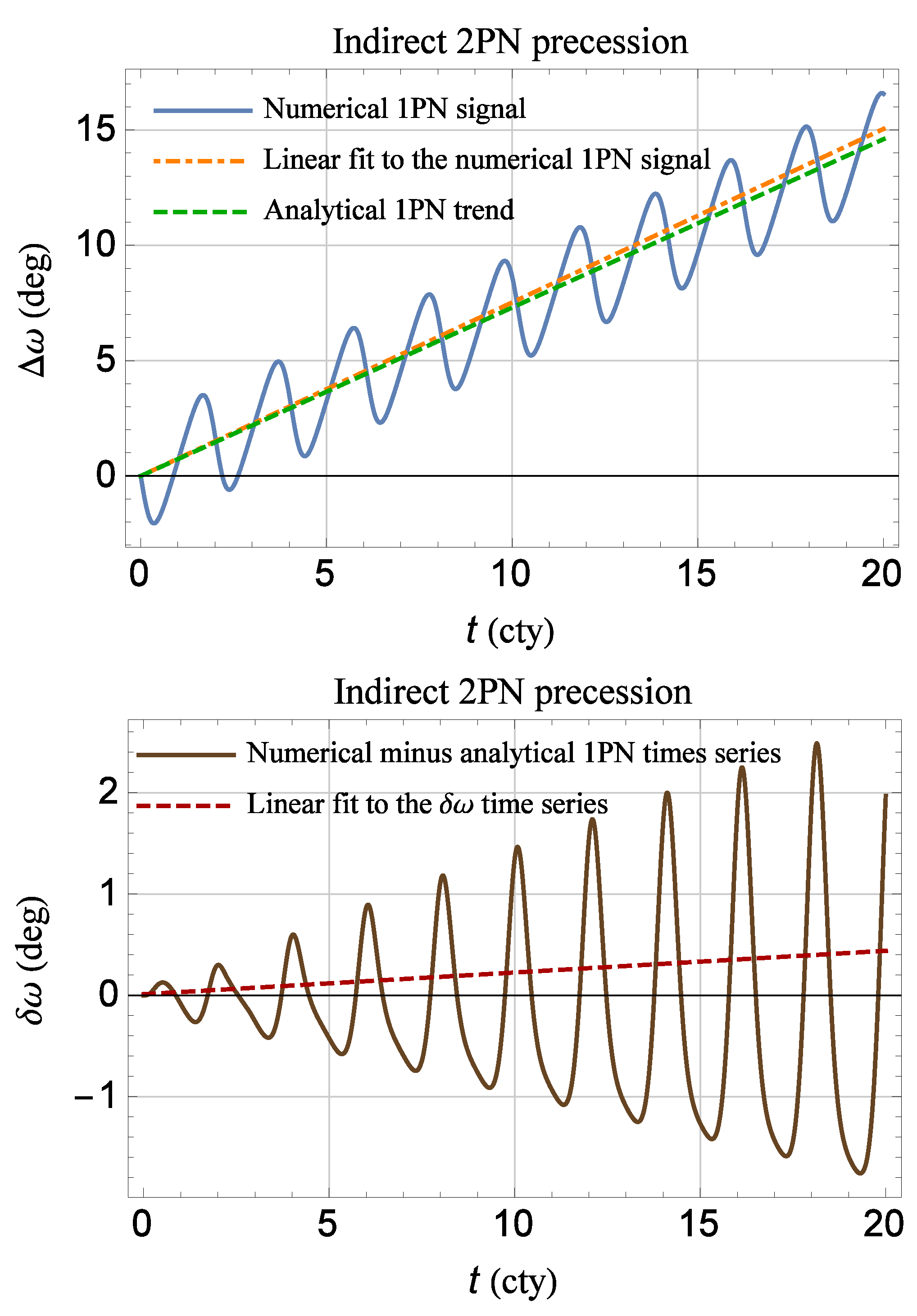
2.2. The Indirect Pericenter Precession due to the 1PN Acceleration

Equation (8), although directly inferred from the 2PN acceleration of Equation (1), does not exhaust the issue of calculating the full pericenter precession to the order O c 4 . Indeed, there are also other two contributions to it, which may be dubbed as “indirect", coming from the well-known 1PN acceleration itself (e.g., [35], p. 332)
A 1 PN = μ c 2 r 2 4 μ r v 2 r ^ + 4 v r v .
Basically, they arise because during an orbital revolution of the test particle under the perturbing influence of A like Equation (10) all the orbital elements, in principle, undergo instantaneous variations changing their values from their fixed Keplerian ones referred to some reference epoch t 0 . Moreover, when the integration over f is performed in order to obtain the net change per orbit, the fact that f is reckoned from a generally varying line of apsides because of A should be taken into account as well. Such features yield additional corrections of the order of O A 2 which, in the present case, are just of the order of O c 4 . We will implement such a strategy by following Iorio [45] in which the indirect effects of order O J 2 c 2 , where J 2 is the primary’s oblateness, were computed in agreement with Will [56,57].
One of the aforementioned indirect contributions to the 2PN pericenter precession, marked conventionally with the superscript I in the following, is obtained from the orbital average of Equations (2) and (3), calculated with Equation (10), by means of the second and third terms of Equation (4) containing just Equation (10) itself which, among other things, shifts slowly the apsidal line from which the true anomaly f is counted. By recalling that the radial, transverse, and out-of-plane components of Equation (10) are ([35], Equation (8.8.5)–(8.8.6), p. 330)
A r 1 PN = μ 2 1 + e cos f 2 3 + e 2 + 2 e cos f 2 e 2 cos 2 f c 2 a 3 1 e 2 3 ,
A τ 1 PN = 4 e μ 2 1 + e cos f 3 sin f c 2 a 3 1 e 2 3 ,
A ν 1 PN = 0 ,
the resulting indirect precession ω ˙ indir 2 PN I of order O c 4 turns out to be
ω ˙ indir 2 PN I = n b μ 2 9 + 37 e 2 + e 4 2 c 4 e 2 a 2 1 e 2 2 .
Please note that Equation (14) is formally singular in the limit e 0 .
The second indirect contribution ω ˙ indir 2 PN II comes from the fact that in general, when an extra-acceleration A like, e.g., Equation (10) enters the equations of motion, all its orbital parameters undergo instantaneous changes during an orbital period. Usually, in standard first order calculations in A, such generally slow variations are neglected by assuming the Keplerian elements as fixed to some fiducial values at a reference epoch t 0 . Instead, accounting also for such changes yield further, indirect effects of the second order in A. The resulting indirect integrated shift over one orbit of any of the orbital elements ϕ i , i = 1 , 5 , where ϕ 1 a , ϕ 2 e , ϕ 3 I , ϕ 4 Ω , ϕ 5 ω , can be calculated as
Δ ϕ i 2 = j = 1 5 f 0 f 0 + 2 π d ϕ i / d f ϕ j K Δ ϕ j f 0 , f 1 d f , i = 1 , 5 ,
where the superscript 2 indicates that the calculation is to the second order in A, K denotes that the content of the curly brackets has to be evaluated onto the unperturbed Keplerian ellipse, and Δ ϕ j f 0 , f 1 , j = 1 , 5 are the instantaneous shifts experienced by the orbital elements during the orbital revolution. The latter ones are calculated as
Δ ϕ j f 0 , f 1 = f 0 f d ϕ j d f K d f , j = 1 , 5 ,
where the superscript 1 indicates that the shifts of Equation (16) are to the first order in A. From [26,53,54,55]
d ω d f = r 2 μ e cos f A r + 1 + r a 1 e 2 sin f A τ cos I d Ω d f + O A 2 ,
valid to the first order in A given, in the present case, by Equation (10), and Equations (11)–(13), it turns out that in the case of pericenter, only the 1PN instantaneous shifts of a and e induced by Equation (10) are required. By recalling that the Gauss equations for such orbital elements, to the first order in A, can be written as [26,53,54,55]
d a d f = 2 a r 2 μ 1 e 2 e A r sin f + p r A τ + O A 2 ,
d e d f = r 2 μ A r sin f + cos f + 1 e 1 r a A τ + O A 2 ,
and that the radial, transverse, and out-of-plane components of Equation (10) are given by Equations (11)–(13), it is straightforward to obtain
Δ a f 0 , f 1 PN = 2 e μ cos f cos f 0 7 + 3 e 2 + 5 e cos f + cos f 0 c 2 1 e 2 2 ,
Δ e f 0 , f 1 PN = μ cos f 0 cos f 3 + 7 e 2 + 5 e cos f + cos f 0 c 2 a 1 e 2 .
They agree with, e.g., Equation (8.8.8) of Soffel & Han [35] (p. 331). Their insertion in Equation (15), calculated for i = 5 by means of Equation (17), yields
ω ˙ indir 2 PN II = n b μ 2 9 87 e 2 136 e 4 + 19 e 6 6 e 3 34 + 26 e 2 cos f 0 + 15 e cos 2 f 0 2 c 4 e 2 a 2 1 e 2 3 .
Please note that also Equation (22) is formally singular in e; moreover, it depends on the initial value of the true anomaly f 0 .
The indirect total 2PN precession ω ˙ indir 2 PN of order O c 4 is the sum of Equation (14) and Equation (22); it reads
ω ˙ indir 2 PN = n b μ 2 5 23 + 20 e 2 4 e 4 + 6 e 34 + 26 e 2 cos f 0 + 15 e cos 2 f 0 2 c 4 a 2 1 e 2 3 .
It should be noticed that Equation (23) is not singular for e 0 . On the other hand, Equation (23) is not univocally determined because of the presence of f 0 . In Section 2.3, we will confirm Equation (23) by numerically integrating the equations of motion for an arbitrary fictitious system.

2.3. A Numerical Confirmation of the Direct and Indirect 2PN Pericenter Precessions

The direct 2PN precession of Equation (8) was successfully confirmed by two numerical integrations of the equations of motion of, say, Mercury in the field of the Sun over 1 century ( cty ) .
It is worthwhile recalling that the present-day level of accuracy in constraining any anomalous perihelion precession of such a planet with the most recent ephemerides, which all model the Solar system dynamics only up to the 1PN level in harmonic coordinates, may be at the level of σ ω ˙ 8 microarcseconds per century (µas cty−1), or, perhaps, 10 50 times worse; see the discussion in Iorio [58], and references therein.
In the first run, we simultaneously integrated the Hermean equations of motion, including the Newtonian monopole and the 2PN acceleration of Equation (1), in rectangular Cartesian coordinates along with the Gauss equations for all the Keplerian orbital elements over a time span 1 cty long starting from a set of initial conditions for the state vector of Mercury retrieved from the WEB interface HORIZONS, maintained by the NASA Jet Propulsion Laboratory (JPL). The resulting time series of the solution for ω t , in blue, is displayed in Figure 1 along with a linear fit to it, in yellow.
The same plot was obtained in a second run in which the Gauss equations were not included in the numerical integration which was limited just to the equations of motion of Mercury in rectangular Cartesian coordinates, all the rest being the same as in the first run. Then, a time series for ω t was straightforwardly computed from the solutions obtained for the Cartesian coordinates x t , y t , z t of the planet by means of the standard conversion formulas for the Keplerian orbital elements. The resulting slope of the fitted linear trend amounts to 2.6 μas cty 1 , in agreement with the first run and Equation (8) calculated with the orbital parameters of Mercury. Interestingly, such a figure is only 3 times smaller than the previously quoted value of σ ω ˙ which, however, as already remarked, may be optimistic by a factor of ≃10–50.
It should be noted that at least in principle, the direct 2PN precession of Equation (8) should be measurable since it is due to a distinct acceleration, i.e., Equation (1), which may be suitably expressed in terms of a dedicated solve-for parameter to be estimated in a least-square sense in some covariance analyses. Instead, the indirect precession of Equation (23), since it comes from the 1PN acceleration of Equation (10) which is routinely modeled in the software of all the teams currently producing the planetary ephemerides, may not be detectable as a separate effect with respect to the other 1PN features of motion. Be that as it may, Equation (23) yields
16 μ as cty 1 ω ˙ indir 2 PN 33 μ as cty 1
for 0 f 0 < 360 deg .
It is possible to numerically confirm our analytical findings also for the indirect 2PN precession in the following way. First of all, a straightforward numerical integration of the equations of motion of a fictitious restricted two-body system to the 1PN level, i.e., by accounting only for the 1PN acceleration of Equation (10), shows that the simple secular trend arising from the celebrated 1PN Einstein-like pericenter precession
ω ˙ 1 PN = 3 n b μ c 2 a 1 e 2
does not match a linear fit to the time series obtained from the numerical integration. This is clearly shown in the upper panel of Figure 2 obtained for, say, f 0 = 0 . It turns out that such a feature lingers even by changing f 0 from a run to another. It is crucial to note that our analytical result for the indirect 2PN precession of Equation (23), calculated with f 0 = 0 , is able to fully explain the discrepancy between the slopes of the simple analytical 1PN trend due to Equation (25) (dashed green line) and of the linear fit (dot-dashed orange line) to the numerically integrated overall signature (continuous blue curve) which, indeed, should include both the direct 1PN and the indirect 2PN effects altogether. It may be shown that it occurs for different values of f 0 as well. Such a feature is further confirmed by a more refined analysis, displayed in the lower panel of Figure 2, consisting of subtracting the well-known analytical instantaneous time series of the 1PN change of ω , given by ([35], Equation (8.8.8), p. 331)
Δ ω ( f 0 , f ) 1 PN = μ 2 c 2 e a 1 e 2 6 e f f 0 + 2 3 + e 2 sin f 5 e sin 2 f 2 3 + e 2 sin f 0 + 5 e sin 2 f 0 ,
from the previously obtained numerical time series for the total (direct 1PN and indirect 2PN) time shift of the pericenter induced by the 1PN acceleration of Equation (10). The resulting time series, obtained by expressing the true anomaly f entering Equation (26) as a function of time t by means of ([26], p. 77)
f t = M t + 2 s = 1 s max 1 s J s s e + j = 1 j max 1 1 e 2 j e j J s j s e + J s + j s e sin s M t ,
where M = n b t t 0 + M 0 is the mean anomaly, M 0 is the mean anomaly at epoch, J k s e is the Bessel function of the first kind of order k, and s max , j max are some values of the summation indexes s , j adequate for the desired accuracy level, is the continuous brown curve for δ ω depicted in the lower panel of Figure 2. It can be noticed that it does not vanish, and a linear fit to it, represented by the dashed red line in the lower panel of Figure 2, returns just the same value as Equation (23). Also, in this case, it occurs by varying f 0 .

3. The Case of a Two-Body System

3.1. The Direct Pericenter Precession due to the 2PN Acceleration

In the case of a two-body system made of two bodies A , B with masses M A , M B , the 2PN acceleration of their relative motion is (see, e.g., [27], Equation (4.4.29), p. 154; [59], Equation (2.2d), p. 825; [60], Equation (B11), p. 10)
A 2 PN = μ c 4 r 2 η 3 + 4 η v 4 + 15 8 η 1 + 3 η v r 4 + η 9 2 6 η v 2 v r 2 + η 13 2 2 η μ r v 2 + + 2 + 25 η + 2 η 2 μ r v r 2 9 + 87 4 η μ 2 r 2 r ^ + η 15 2 + 2 η v 2 η 9 2 + 3 η v r 2 2 + 41 2 η + 4 η 2 μ r v r v .
where μ G M , M M A + M B , and η M A M B / M 2 .
The direct 2PN precession ω ˙ dir 2 PN of the pericenter of the relative motion of a two-body system can be straightforwardly computed from Equation (28) in the same fashion as for the point particle treated in Section 2.1. The radial, transverse, and out-of-plane components of Equation (28) are
64 c 4 1 e 2 4 a 5 n b 6 1 + e cos f 2 A r 2 PN = e 4 η 39 + 191 η + 16 36 + η 73 + 8 η + + 8 e 2 36 + η 13 + 72 η + + 8 e 144 + η 288 + 80 η + e 2 13 + 92 η cos f + + e 2 4 72 + η 298 + 144 η + e 2 45 + 11 η cos 2 f + + e η 8 57 + 20 η cos 3 f + 3 e 17 + 7 η cos 4 f ,
A τ 2 PN = a 5 e n b 6 1 + e cos f 3 sin f 2 c 4 1 e 2 4 4 + η 26 + 4 η e 2 15 + 4 η +
+ e 4 + 11 η cos f + 3 e 2 η 3 + 2 η sin 2 f ,
A ν 2 PN = 0 ;
they reduce to Equations (5)–(7) in the point particle limit, i.e., for η 0 . By averaging the right-hand sides of Equations (1) and (2), calculated with Equations (29)–(31), with the first term of Equation (4) one finally obtains
ω ˙ dir 2 PN = n b μ 2 e 2 2 + 3 7 16 η η + 8 7 + 5 7 η η 8 c 4 a 2 1 e 2 2 .
Equation (32) reduces to Equation (8) for η 0 .
For the double pulsar PSR J0737–3039A/B, characterized by [61] M A = 1.3381 M , M B = 1.2489 M , η = 0.249 , M = 2.58708 M , a = 878960 km , e = 0.0877 , P b = 0.10 d , Equation (32) yields
ω ˙ dir 2 PN = 0.00019 deg yr 1 .
The current accuracy in measuring the periastron precession of the double pulsar is [61]
σ ω ˙ = 0.00068 deg yr 1 .
An accuracy level of the order of Equation (33) should be reached in the forthcoming years thanks to new telescopes [62]. For the historical binary pulsar PSR B1913+16, whose relevant physical and orbital parameters are [63] M A = 1.4398 M , M B = 1.3886 M , η = 0.249 , M = 2.8284 M , a = 1.949 × 10 6 km , e = 0.6171334 , P b = 0.32 d , Equation (32) returns
ω ˙ dir 2 PN = 0.000038 deg yr 1 ,
while the most recent determination of its periastron rate is accurate to [63]
σ ω ˙ = 0.000005 deg yr 1 .
For the supermassive binary black hole in OJ 287, whose relevant orbital parameters are [38] M A = 18438 × 10 6 M , M B = 150.13 × 10 6 M , P b = 12.06 yr , e = 0.657 , Equation (32) predicts a direct 2PN perinigricon2 precession as large as ω ˙ dir 2 PN = 11.0 deg cty 1 , a remarkable fraction of the 1PN rate of change
ω ˙ 1 PN = 3 n b μ c 2 a 1 e 2 = 206.8 deg cty 1
corresponding to a shift per orbit
Δ ω 1 PN = 24.9 deg .

3.2. The Indirect Pericenter Precession Due to the 1PN Acceleration

The indirect precession due to the 1PN acceleration (see, e.g., [27], Equation (4.4.28), p. 154; [34], Equation (A2.6), p. 166; [35], Equation (10.3.7), p. 381)
A 1 PN = μ c 2 r 2 4 + 2 η μ r + 3 2 η v r 2 1 + 3 η v 2 r ^ + 4 2 η v r v
can be calculated as in the point particle case treated in Section 2.2.
The radial, transverse, and out-of-plane components of Equation (39) are
A r 1 PN = μ 2 1 + e cos f 2 e 2 4 13 η 4 3 + η + 8 e 1 2 η cos f + e 2 8 + η cos 2 f 4 c 2 a 3 1 e 2 3 ,
A τ 1 PN = 2 e μ 2 1 + e cos f 3 2 η sin f c 2 a 3 1 e 2 3 ,
A ν 1 PN = 0 .
Equations (40)–(42), which agree with Equations (A2.77a)–(A2.77c) of (Soffel [34], p. 178), reduce to Equations (11)–(13) for η 0 .
The indirect precession ω ˙ indir 2 PN I due to the second and third terms of Equation (4) turns out to be
ω ˙ indir 2 PN I = n b μ 2 32 3 + η 2 + 8 e 2 148 + 5 η 43 + 17 η + e 4 32 + 3 η 56 + 75 η 64 c 4 e 2 a 2 1 e 2 2 .
Equation (43) reduces to Equation (14) in the point particle limit.
The 1PN instantaneous shifts of a and e induced by Equation (39) are
Δ a f 0 , f 1 PN = e μ cos f cos f 0 2 c 2 1 e 2 2 4 7 + 3 η + e 2 3 + 4 η + + e e η cos 2 f + 4 5 + 4 η cos f 0 + 2 cos f 10 + 8 η + e η cos f 0 + + e η cos 2 f 0 , ,
Δ e f 0 , f 1 PN = μ cos f cos f 0 4 c 2 a 1 e 2 4 3 + η + e 2 7 + 6 η + + e e η cos 2 f + 4 5 + 4 η cos f 0 + 2 cos f 10 + 8 η + e η cos f 0 + + e η cos 2 f 0 .
They agree with Equations (1) and (2) of (Soffel [34], p. 178), and reduce to Equations (20) and (21) in the limit η 0 . Equations (44) and (45) allow computation of the other indirect contribution ω ˙ indir 2 PN II to the 2PN precession, which reads
64 c 4 e 2 a 2 1 e 2 3 n b μ 2 ω ˙ indir 2 PN II = 32 3 + η 2 8 e 2 3 + η 116 + 47 η + + e 4 4352 + 10664 4183 η η + + e 6 608 + 3 304 601 η η + + 48 e 3 8 17 + 7 η + e 2 104 + 109 η cos f 0 + + 3 e 4 5 + 4 η cos 2 f 0 + e η cos 3 f 0 .
The sum of Equation (43) and Equation (46), which reduces to Equation (22) for η 0 , yields the total indirect 2PN precession, which is
32 c 4 a 2 1 e 2 3 n b μ 2 ω ˙ indir 2 PN = e 4 320 + 540 η 789 η 2 16 115 + 16 η 7 + 2 η 4 e 2 400 + η 1097 + 466 η + + 24 e 8 17 + 7 η + e 2 104 + 109 η cos f 0 + + 3 e 4 5 + 4 η cos 2 f 0 + e η cos 3 f 0 .
Equation (47) agrees with Equation (23) in the point particle limit.
According to Equation (47), the indirect periastron precession of PSR J07373039A/B lies in the range
0.00092 deg yr 1 ω ˙ indir 2 PN 0.00132 deg yr 1
for 0 f 0 < 360 deg . If summed to the direct precession of Equation (33), such a result would bring the total 2PN periastron precession of the double pulsar in the realm of measurability independently of f 0 . For the binary pulsar PSR B1913+16, the indirect 2PN precession of Equation (47) is
0.000048 deg yr 1 ω ˙ indir 2 PN 0.001052 deg yr 1
for 0 f 0 < 360 deg . This implies that, for certain values of f 0 , Equation (49) may cancel the direct precession of Equation (35), thus making a potential measurement of the 2PN orbital effect unmeasurable. For OJ 287, Equation (47) yields an indirect 2PN perinigricon precession ranging from a maximum of 516 deg cty 1 to a minimum of 20 deg cty 1 . It is a remarkable result in view of Equation (37).

4. A Comparison with Other Works

To the knowledge of the present author, the only other work in the literature making use of the method of the variation of constants and the Gauss equations is Kopeikin & Potapov [12]. As we will show, their result is incorrect because of the treatment of what are dubbed here as indirect effects.
Equation (5.2) of Kopeikin & Potapov [12], which we reproduce here to the benefit of the reader, is their main result. It is the total 2PN pericenter shift per orbit, in units of 2 π , written in terms of the constants of integration k 1 , k 2 of the solutions of the Gauss equations for the semimajor axis and the eccentricity to the 1PN level. In our notation3, it is, in the test particle case,
Δ ω tot 2 PN 2 π = 3 μ c 2 k 1 1 k 2 2 1 + 3 μ 4 c 2 k 1 1 k 2 2 μ 4 c 2 k 1 .
Since the constants of integrations k 1 , k 2 entering Equation (50) are determined with the initial conditions at t = t 0 , they contain explicitly f 0 ; thus, Equation (5.2) of Kopeikin & Potapov [12] actually does depend on the latter one, contrary to what, at first glance, someone could argue, perhaps mislead by the notation used by Kopeikin & Potapov [12] for k 1 , k 2 . By retrieving the explicit expression of k 1 , k 2 from Eqautions (20) and (21)
k 1 = a + e μ 14 + 6 e 2 cos f 0 + e 4 + 5 cos 2 f 0 c 2 1 e 2 2 ,
k 2 = e + μ 6 + 14 e 2 cos f 0 + e 2 + 5 cos 2 f 0 2 c 2 a 1 e 2 ,
where a and e entering Equations (51) and (52) are intended as the Keplerian values of the unperturbed case, Equation (5.2) of Kopeikin & Potapov [12] can be finally cast into the form
Δ ω tot 2 PN 2 π = 3 μ 2 2 + e 2 32 e 2 cos f 0 4 c 4 a 2 1 e 2 2 ,
which does not agree with the corresponding expression for Δ ω tot 2 PN / 2 π obtainable from the sum of our Equation (8) and Equation (23) by taking its ratio to n b .
From what can be deduced from the description of the method followed by Kopeikin & Potapov [12], the indirect effect corresponding to our ω ˙ indir 2 PN ( II ) arises from the replacement a a + Δ a f 0 , f 1 PN , e e + Δ e f 0 , f 1 PN in4 Equation (17), in a series expansion of it in powers of c 1 to the order c 4 , and in an integration of the resulting expression from f 0 to f 0 + 2 π . The result, not explicitly shown by Kopeikin & Potapov [12], is
Δ ω indir 2 PN ( II ) 2 π = μ 2 9 48 e 2 + e 4 48 e 3 cos f 0 2 c 4 a e 2 1 e 2 2 ,
which does not agree with the corresponding expression from our Equation (22) for ω ˙ indir 2 PN ( II ) . Instead, it seems that the other two contributions arising from Equation (5.1) of Kopeikin & Potapov [12], despite not explicitly displayed by Kopeikin & Potapov [12], agree with the corresponding shifts from our Equation (8) and Equation (14) because their sum with Equation (54) yields just Equation (53). In particular, the fractional 2PN advance per orbit, which should come from the first term of Equation (5.1) of Kopeikin & Potapov [12] calculated with A 2 PN onto a reference Keplerian ellipse, is not shown; nonetheless, from the description of the calculational method by Kopeikin & Potapov [12], one may expect that it agrees with our Equation (8). Moreover, a direct calculation confirms that the second term of Equation (5.1) of Kopeikin & Potapov [12] yields just the shift corresponding to our Equation (14) for ω ˙ indir 2 PN ( I ) . Thus, it can be inferred that the total indirect 2PN pericenter precession of Kopeikin & Potapov [12] can be cast into the form
ω ˙ indir 2 PN = n b μ 2 11 + 2 e 2 48 e cos f 0 2 c 4 a 2 1 e 2 2 .
It neatly disagrees with our numerical results of Section 2.3 since, for the fictitious system treated in Figure 2, Equation (55) provides a slope as little as 0.00255 deg cty 1 .
It may be interesting to make a comparison of our results also with the seminal results by Damour & Schafer [5], despite they did not use the Gauss equations. Damour & Schafer [5], following the example by Landau & Lifshitz [65], started from the Hamiltonian of the binary system in Arnowitt–Deser–Misner (ADM) coordinates [66] and adopted the Hamilton-Jacobi method. As far as the 2PN pericenter precession of a system of two mass monopoles is concerned, their main result is Equation (3.12)
Δ ω tot 2 PN 2 π = 3 c 2 h 2 1 + 5 2 η E c 2 + 35 4 5 2 η 1 c 2 h 2 ,
where h and E are the coordinate-invariant, reduced orbital angular momentum and energy, respectively. Its translation in terms of the parameters of the Damour–Deruelle (DD) parametrization [67] is given by Equation (5.18) of Damour & Schafer [5]
Δ ω tot 2 PN 2 π = 3 μ n 2 / 3 c 2 1 e t 2 1 + μ n 2 / 3 c 2 1 e t 2 39 4 x A 2 + 27 4 x B 2 + 15 x A x B μ n 2 / 3 c 2 13 4 x A 2 + 1 4 x B 2 + 13 3 x A x B
where n is the PN mean motion ([67], Equation (3.6d) )
n = 2 E 3 / 2 μ 1 E 4 c 2 η 15 ,
x A M A M , x B M B M = 1 x A ,
and e t is one of the DD parameters [67]. Expressing Equation (56) in terms of the osculating Keplerian orbital elements can be made in the following two steps. First, E , h are to be written in terms of the DD parameters a r , e r by inverting Equations (3.6a) and Equation (3.6b) of Damour & Deruelle [67]. The result is
E = μ 2 a r 1 1 + μ 4 c 2 a r 7 η ,
h 2 = a r 1 e r 2 + μ 2 c 2 19 + e r 2 7 + η 3 η μ 2 16 c 4 a r 577 + e r 2 7 + η 2 + 246 25 η η μ 1 + μ 2 c 2 a r 11 3 η .
Then, Equations (28) to (29) of Klioner & Kopeikin [24], which in general relativity, are
a r = a 1 e 2 2 d a 0 1 e 2 2 μ c 2 3 + η + e 2 13 + e 2 + 7 η + 2 e 2 η 1 e 2 2 ,
e r = 2 a d e 0 e 1 + e 2 + e μ c 2 17 + 6 η + e 2 2 + 4 η 2 a 1 + e 2 ,
with the aid of Equation (14) and Equation (16) of Klioner & Kopeikin [24], whose general relativistic expressions are
d a 0 = e μ 8 7 + 3 η + e 2 24 + 31 η cos f 0 + e 4 5 + 4 η cos 2 f 0 + e η cos 3 f 0 4 c 2 1 e 2 2 ,
d e 0 = μ 8 3 + η + e 2 56 + 47 η cos f 0 + e 4 5 + 4 η cos 2 f 0 + e η cos 3 f 0 8 c 2 a 1 + e 2 ,
are used to express a r , e r as functions of the osculating Keplerian elements a , e . We obtain for a r a , e , e r a , e
4 1 e 2 2 a r = 4 a 1 e 2 2 μ c 2 3 + η + e 4 1 + 2 η + e 2 13 + 7 η + + e μ c 2 56 + e 2 24 31 η 24 η cos f 0 + + e 4 5 4 η cos 2 f 0 e η cos 3 f 0 ,
8 a 1 + e 2 e r = 4 e 2 a 1 + e 2 + μ c 2 17 + 6 η + e 2 2 + 4 η + + μ c 2 8 3 + η + e 2 56 + 47 η cos f 0 + + e 4 5 + 4 η cos 2 f 0 + e η cos 3 f 0 .
Finally, an expansion of the obtained expression in powers of c 1 to the 2PN level yields, in the point particle limit, Equation (53) which, as already noted, is incorrect. On the other hand, Equation (56) and Equation (57) seem to be mutually inconsistent since their expressions in terms of a , e do not even agree each other. Indeed, by using Equations (58), (66) and (67), Equation (30) of Klioner & Kopeikin [24], which, in general relativity, reads
e t = 2 a d e 0 e 1 + e 2 + e μ c 2 3 3 + η + e 2 6 + 7 η 2 a 1 + e 2 ,
and Equation (65) to express e t in terms of a , e
8 a 1 + e 2 e t = 4 e 2 a 1 + e 2 + μ c 2 3 3 + η + e 2 6 + 7 η + + μ c 2 8 3 + η + e 2 56 + 47 η cos f 0 + + e 4 5 + 4 η cos 2 f 0 + e η cos 3 f 0 ,
one obtains, in the limit η 0 ,
Δ ω tot 2 PN 2 π = 3 μ 2 2 3 e 2 32 e cos f 0 4 c 4 a 2 1 e 2 2 ,
which disagrees even with Equation (53) itself. By expanding Equations (53) and (70) in powers of e, it turns out that their disagreement is at the order O e 2 .

5. Summary and Conclusions

We analytically worked out the 2PN secular pericenter precession ω ˙ 2 PN of both a test particle orbiting a static central body and a full two-body system made of a pair of comparable non-rotating monopole masses with the method of variation of orbital elements.
We, first, calculated the direct precession ω ˙ dir 2 PN induced by the 2PN acceleration entering the equations of motion written in harmonic coordinates. Two different numerical integrations of the equations of motion of a point particle confirmed our analytical results. For Mercury moving in the field of Sun, it is ω ˙ dir 2 PN = 2.6 μas cty−1. It is just 3 times smaller than the present-day formal accuracy σ ω ˙ = 8 μas cty−1 in constraining any unmodeled effect in the Hermean perihelion rate with the latest planetary ephemerides, although σ ω ˙ may be realistically up to ≃10–50 times worse. In the case of the binary pulsar PSR B1913+16, the direct 2PN periastron rate is ω ˙ dir 2 PN = 0.000038 deg yr 1 , to be compared with the most recent determination of its periastron rate σ ω ˙ = 0.000005 deg yr 1 , while for the double pulsar PSR J0737–3039A/B one has ω ˙ dir 2 PN = 0.00019 deg yr 1 and σ ω ˙ = 0.00068 deg yr 1 . The direct 2PN perinigricon precession of the supermassive binary black hole in OJ 287 amounts to 11 deg cty 1 .
Then, we computed also the indirect 2PN pericenter precession ω ˙ indir 2 PN arising from the fact that the 1PN acceleration actually changes instantaneously the semimajor axis and the eccentricity, and shifts the line of apsides instant by instant during one full orbital revolution. If properly accounted for in the orbital average, such features, which are of the second order in the acceleration causing them, gives rise to a further contribution of order O c 4 to the 2PN pericenter precession which adds on the direct one. The resulting expression turns out to be dependent on the initial position f 0 along the orbit. Numerical integrations of the equations of motion confirmed also such a result. Since the orbital dynamics of our Solar system is routinely modeled up to the 1PN level in harmonic coordinates of PN theory, it is unlikely that such an indirect precession can be measured separately because it does not come from a distinct acceleration which, instead, could be suitably expressed in terms of a dedicated solve-for parameter to be estimated in specific covariance analyses. For Mercury, its nominal size amounts to 16–33 μas cty−1, depending on f 0 . For the binary pulsars, the experimental approach is different. It implies the determination, in a phenomenological, model-independent way, of several post-Keplerian parameters, among which there is also the periastron precession, from a confrontation of an analytical timing formula with the recorded pulses. Then, model-dependent analytical expressions for the measured post-Keplerian effects are used to determine the masses of the system, and to perform one or more tests of the model of gravitation considered. In the case of PSR B1913+16, the indirect 2PN precession ranges from 0.000048 deg yr 1 to 0.001052 deg yr 1 , while for PSR J07373039A/B it is 0.00092–0.00132 deg yr 1 . This shows that the choice of f 0 may enhance or even cancel out the overall 2PN periastron precession. For OJ 287, it ranges from 20 deg cty 1 to 516 deg cty 1 ; the 1PN perinigricon precession amounts to 206.8 deg cty 1 .
We compared our formulas to some other analytical results in the literature by showing that the latter ones disagree with ours and with our numerical integrations of the equations of motion. It appears that the source of discrepancy relies in the treatment of the indirect effects arising from the inclusion of the instantaneous 1PN changes of the semimajor axis and eccentricity in the integration over one orbital revolution of the pericenter shift due to the 1PN acceleration itself.

Funding

This research received no external funding.

Acknowledgments

I am grateful to all the referees and the Editorial Board’s members who took part in the reviewing process for their patience and constructive comments which notably improved the manuscript.

Conflicts of Interest

The authors declare no conflict of interest.

References

  1. Debono, I.; Smoot, G.F. General relativity and cosmology: Unsolved questions and future directions. Universe 2016, 2, 23. [Google Scholar] [CrossRef]
  2. Bagchi, M. Periastron advance in neutron star–black hole binaries. Mon. Not. R. Astron. Soc. 2013, 428, 1201. [Google Scholar] [CrossRef] [Green Version]
  3. Blanchet, L. Gravitational radiation from post-Newtonian sources and inspiralling compact binaries. Living Rev. Relat. 2014, 17, 2. [Google Scholar] [CrossRef] [PubMed] [Green Version]
  4. Damour, T.; Schaefer, G. Le problème des deux corps en relativité générale. CR Acad. Sci. Sér. II 1987, 305, 839. [Google Scholar]
  5. Damour, T.; Schafer, G. Higher-order relativistic periastron advances and binary pulsars. Nuovo Cimento B 1988, 101, 127. [Google Scholar] [CrossRef]
  6. D’Eliseo, M.M. Higher-order corrections to the relativistic perihelion advance and the mass of binary pulsars. Astrophys. Space Sci. 2011, 332, 121. [Google Scholar] [CrossRef] [Green Version]
  7. Do-Nhat, T. Full asymptotic expansion of the relativistic orbit of a test particle under the exact Schwarzschild metric. Phys. Lett. A 1998, 238, 328. [Google Scholar] [CrossRef]
  8. Gergely, L.A.; Keresztes, Z. Spinning compact binary dynamics and chameleon orbits. Phys. Rev. D 2015, 91, 024012. [Google Scholar] [CrossRef] [Green Version]
  9. Heng, F.; Zhao, F. Exact analytical solution to equations of perihelion advance in general relativity. Int. J. Theor. Phys. 2009, 48, 2198–2204. [Google Scholar]
  10. Hoenselaers, C. On Quadrupole Effects on Planetary Orbits Prog. Theor. Phys. 1976, 56, 324. [Google Scholar] [CrossRef] [Green Version]
  11. Königsdörffer, C.; Gopakumar, A. Post-Newtonian accurate parametric solution to the dynamics of spinning compact binaries in eccentric orbits: The leading order spin-orbit interaction. Phys. Rev. D 2005, 71, 024039. [Google Scholar] [CrossRef] [Green Version]
  12. Kopeikin, S.M.; Potapov, V.A. Relativistic shift of the periastron of a double pulsar in the post-post-Newtonian approximation of General Relativity. Astron. Rep. 1994, 38, 104. [Google Scholar]
  13. Mak, M.K.; Leung, C.S.; Harko, T. Computation of the General Relativistic Perihelion Precession and of Light Deflection via the Laplace-Adomian Decomposition Method. Adv. High Energy Phys. 2018, 2018, 7093592. [Google Scholar] [CrossRef]
  14. Marín, C.; Poveda, J. Perihelion precession in binary systems: Higher order corrections. Astrophys. Space Sci. 2018, 363, 245. [Google Scholar] [CrossRef] [Green Version]
  15. Memmesheimer, R.-M.; Gopakumar, A.; Schäfer, G. Third post-Newtonian accurate generalized quasi-Keplerian parametrization for compact binaries in eccentric orbits. Phys. Rev. D 2004, 70, 104011. [Google Scholar] [CrossRef] [Green Version]
  16. Ohta, T.; Kimura, T. Launch window study for the highly eccentric orbit satellite HEOS-1. Prog. Theor. Phys. 1989, 81, 679. [Google Scholar] [CrossRef] [Green Version]
  17. Schäfer, G.; Wex, N. Second post-Newtonian motion of compact binaries. Phys. Lett. A 1993, 174, 196. [Google Scholar] [CrossRef]
  18. Schäfer, G.; Wex, N. Errata: Second post-Newtonian motion of compact binaries. Phys. Lett. A 1993, 177, 461. [Google Scholar] [CrossRef]
  19. Tucker, A.; Will, C.M. Pericenter advance in general relativity: Comparison of approaches at high post-Newtonian orders. Class. Quantum Gravity 2019, 36, 115001. [Google Scholar] [CrossRef] [Green Version]
  20. Walters, S.J. A simple exact series representation for relativistic perihelion advance. Mon. Not. R. Astron. Soc. 2018, 480, 3747. [Google Scholar] [CrossRef]
  21. Wex, N. The second post-Newtonian motion of compact binary-star systems with spin. Class. Quantum Gravity 1995, 12, 983. [Google Scholar] [CrossRef]
  22. Will, C.M. New general relativistic contribution to mercury’s perihelion advance. Phys. Rev. Lett. 2018, 120, 191101. [Google Scholar] [CrossRef] [PubMed] [Green Version]
  23. Will, C.M.; Maitra, M. Relativistic orbits around spinning supermassive black holes: Secular evolution to 4.5 post-Newtonian order. Phys. Rev. D 2017, 95, 064003. [Google Scholar] [CrossRef] [Green Version]
  24. Klioner, S.A.; Kopeikin, S.M. The post-Keplerian orbital representations of the relativistic two-body problem. Astrophys. J. 1994, 427, 951. [Google Scholar] [CrossRef]
  25. Bertotti, B.; Farinella, P.; Vokrouhlický, D. Physics of the Solar System; Springer: Dordrecht, The Netherlands, 2003. [Google Scholar]
  26. Brouwer, D.; Clemence, G.M. Methods of Celestial Mechanics; Academic Press: New York, NY, USA, 1961. [Google Scholar]
  27. Brumberg, V.A. Essential Relativistic Celestial Mechanics; Adam Hilger: Bristol, UK, 1991. [Google Scholar]
  28. Danby, J.M.A. Fundamentals of Celestial Mechanics; The Macmillan Company: New York, NY, USA, 1962. [Google Scholar]
  29. Kopeikin, S.; Efroimsky, M.; Kaplan, G. Relativistic Celestial Mechanics of the Solar System; Wiley-VCH: Weinheim, Germany, 2011. [Google Scholar]
  30. Murray, C.D.; Dermott, S.F. Solar System Dynamics; Cambridge Univ. Press: Cambridge, UK, 2000. [Google Scholar]
  31. Plummer, H.C. An Introductory Treatise in Dynamical Astronomy; Dover Publications, Inc.: New York, NY, USA, 1960. [Google Scholar]
  32. Poisson, E.; Will, C.M. Gravity; Cambridge University Press: Cambridge, UK, 2014. [Google Scholar]
  33. Roy, A.E. Orbital Motion; Institute of Physics Publishing: Bristol, UK, 2005. [Google Scholar]
  34. Soffel, M.H. Relativity in Astrometry, Celestial Mechanics and Geodesy; Springer: Heidelberg, Gremany, 1989. [Google Scholar]
  35. Soffel, M.H.; Han, W.-B. Applied General Relativity; Springer: Cham, Switzerland, 2019. [Google Scholar]
  36. Tisserand, F. Traité de Mécanique Céleste; Gauthier-Villars: Paris, France, 1989. [Google Scholar]
  37. Dey, L.; Gopakumar, A.; Valtonen, M.; Zola, S.; Susobhanan, A.; Hudec, R.; Pihajoki, P.; Pursimo, T.; Berdyugin, A.; Piirola, V.; et al. The Unique Blazar OJ 287 and Its Massive Binary Black Hole Central Engine. Universe 2019, 5, 108. [Google Scholar] [CrossRef] [Green Version]
  38. Dey, L.; Valtonen, M.J.; Gopakumar, A.; Zola, S.; Hudec, R.; Pihajoki, P.; Ciprini, S.; Matsumoto, K.; Sadakane, K.; Kidger, M.; et al. Authenticating the presence of a relativistic massive black hole binary in OJ 287 using its general relativity centenary flare: Improved orbital parameters. Astrophys. J. 2018, 866, 11. [Google Scholar] [CrossRef] [Green Version]
  39. Frutos-Alfaro, F.; Soffel, M. On relativistic multipole moments of stationary space–times. R. Soc. Open Sci. 2018, 5, 180640. [Google Scholar] [CrossRef] [Green Version]
  40. Heimberger, J.; Soffel, M.; Ruder, H. Relativistic effects in the motion of artificial satellites: The oblateness of the central body II. Celest. Mech. Dyn. Astron. 1990, 47, 205. [Google Scholar] [CrossRef]
  41. Meichsner, J.; Soffel, M.H. Effects on satellite orbits in the gravitational field of an axisymmetric central body with a mass monopole and arbitrary spin multipole moments. Celest. Mech. Dyn. Astron. 2015, 123, 1. [Google Scholar] [CrossRef] [Green Version]
  42. Panhans, M.; Soffel, M.H. Gravito-magnetism of an extended celestial body. Class. Quantum Gravity 2014, 31, 245012. [Google Scholar] [CrossRef]
  43. Schanner, M.; Soffel, M. Relativistic satellite orbits: Central body with higher zonal harmonics. Celest. Mech. Dyn. Astron. 2018, 130, 40. [Google Scholar] [CrossRef]
  44. Soffel, M.; Wirrer, R.; Schastok, J.; Ruder, H.; Schneider, M. Relativistic effects in the motion of artificial satellites: The oblateness of the central body I. Celest. Mech. Dyn. Astron. 1987, 42, 81. [Google Scholar] [CrossRef]
  45. Iorio, L. Post-Newtonian direct and mixed orbital effects due to the oblateness of the central body. Int. J. Mod. Phys. D 2015, 24, 1550067. [Google Scholar] [CrossRef] [Green Version]
  46. Fienga, A.; Deram, P.; Viswanathan, V.; Di Ruscio, A.; Bernus, L.; Durante, D.; Gastineau, M.; Laskar, J. INPOP19a Planetary Ephemerides. Available online: https://hal.archives-ouvertes.fr/hal-02470929/document (accessed on 11 April 2020).
  47. Folkner, W.M.; Williams, J.G.; Boggs, D.H.; Park, R.S.; Kuchynka, P. The planetary and lunar ephemerides DE430 and DE431. Interplanet. Netw. Prog. Rep. 2014, 42, 1. [Google Scholar]
  48. Pitjeva, E.V.; Pitjev, N.P. Masses of the Main Asteroid Belt and the Kuiper Belt from the Motions of Planets and Spacecraft. Astron. Lett. 2018, 44, 554. [Google Scholar] [CrossRef] [Green Version]
  49. Hulse, R.A.; Taylor, J.H. Discovery of a pulsar in a binary system. Astrophys. J. 1875, 195, L51. [Google Scholar] [CrossRef]
  50. Burgay, M.; D’Amico, N.; Possenti, A.; Manchester, R.N.; Lyne, A.G.; Joshi, B.C.; McLaughlin, M.A.; Kramer, M.; Sarkissian, J.M.; Camilo, F. et al. An increased estimate of the merger rate of double neutron stars from observations of a highly relativistic system. Nature 2003, 426, 531. [Google Scholar] [CrossRef]
  51. Lyne, A.G.; Burgay, B.; Kramer, M.; Possenti, A.; Manchester, R.N.; Camilo, F.; McLaughlin, M.A.; Lorimer, D.R.; D’Amico, N.; Joshi, B.C.; et al. A double-pulsar system: A rare laboratory for relativistic gravity and plasma physics. Science 2004, 303, 1153. [Google Scholar] [CrossRef] [Green Version]
  52. Egorov, V.A. Definition of the True Anomaly in Perturbed Motion. Sov. Astron. 1958, 2, 147. [Google Scholar]
  53. Mioc, V.; Radu, E. Perturbations in the Anomalistic Period of Artificial Satellites Caused by the Direct Solar Radiation Pressure Centre for Astronomy and Space Sciences, Satellite Tracking Station No. 1132. Astron. Nachr. 1979, 300, 313. [Google Scholar] [CrossRef]
  54. Roth, E.A. Launch window study for the highly eccentric orbit satellite HEOS-1. Celest. Mech. 1970, 2, 369. [Google Scholar] [CrossRef]
  55. Taratynova, G.P. Über die Bewegung von künstlichen Satelliten im nicht-zentralen Schwerefeld der Erde unter Berücksichtigung des Luftwiderstandes. Fortschr. Phys. 1959, 7, 55. [Google Scholar] [CrossRef]
  56. Will, C.M. Incorporating post-Newtonian effects in N-body dynamics. Phys. Rev. D 2014, 89, 044043. [Google Scholar] [CrossRef] [Green Version]
  57. Will, C.M. Erratum: Incorporating post-Newtonian effects in N-body dynamics. Phys. Rev. D 2015, 91, 029902. [Google Scholar] [CrossRef] [Green Version]
  58. Iorio, L. Calculation of the Uncertainties in the Planetary Precessions with the Recent EPM2017 Ephemerides and their Use in Fundamental Physics and Beyond. Astrophys. J. 2019, 157, 220. [Google Scholar] [CrossRef] [Green Version]
  59. Kidder, L.E. Coalescing binary systems of compact objects to (post)5/2–Newtonian order. V. Spin effects. Phys. Rev. D 1995, 52, 821. [Google Scholar] [CrossRef] [PubMed] [Green Version]
  60. Gergely, L.A. Spinning compact binary inspiral. II. Conservative angular dynamics. Phys. Rev. D 2010, 82, 104031. [Google Scholar] [CrossRef] [Green Version]
  61. Kramer, M.; Stairs, I.H.; Manchester, R.N.; McLaughlin, M.A.; Lyne, A.G.; Ferdman, R.D.; Burgay, M.; Lorimer, D.R.; Possenti, A.; D’Amico, N.; et al. Tests of general relativity from timing the double pulsar. Science 2006, 314, 97. [Google Scholar] [CrossRef] [Green Version]
  62. Kehl, M.S.; Wex, N.; Kramer, M.; Liu, K. Future measurements of the Lense-Thirring effect in the Double Pulsar. In Proceedings of the Fourteenth Marcel Grossmann Meeting On Recent Developments in Theoretical and Experimental General Relativity, Astrophysics, and Relativistic Field Theories, Rome, Italy, 12–18 July 2015; Bianchi, M., Jansen, R.T., Ruffini, R., Eds.; World Scientific: Singapore, 2017; Volume 4, pp. 1860–1865. [Google Scholar]
  63. Weisberg, J.M.; Nice, D.J.; Taylor, J.H. Timing measurements of the relativistic binary pulsar PSR B1913+ 16. Astrophys. J. 2010, 722, 1030. [Google Scholar] [CrossRef]
  64. Schödel, R.; Ott, T.; Genzel, R.; Hofmann, R.; Lehnert, M.; Eckart, A.; Mouawad, N.; Alexander, T.; Reid, M.J.; Lenzen, R.; et al. A star in a 15.2-year orbit around the supermassive black hole at the centre of the Milky Way. Nature 2002, 419, 694. [Google Scholar] [CrossRef] [PubMed]
  65. Landau, L.D.; Lifshitz, E.M. The Classical Theory of Fields; Pergamon Press: Oxford, UK, 1971. [Google Scholar]
  66. Arnowitt, R.; Deser, S.; Misner, C.W. Gravitational-electromagnetic coupling and the classical self-energy problem. Phys. Rev. 1960, 120, 313. [Google Scholar] [CrossRef]
  67. Damour, T.; Deruelle, N. General relativistic celestial mechanics of binary systems. I. The post-Newtonian motion. Ann. Inst. Henri Poincaré Phys. Théor. 1985, 43, 107. [Google Scholar]
1.
For the sake of simplicity, we will omit the brackets denoting the average over one orbital revolution here and throughout the paper.
2.
It is one of the possible names which can be attributed to the pericenter when black holes are involved [64]. It comes from the Latin word “niger”, meaning “black”.
3.
In Kopeikin & Potapov [12], it is k 1 a 0 , k 2 e 0 .
4.
It is done in the first term of Equation (5.1) of Kopeikin & Potapov [12] when Equation (3.6) of Kopeikin & Potapov [12] for d ω / d t is calculated to the 1PN level.
Figure 1. Numerically produced time series, in blue, of the 2PN evolution of the perihelion ω of Mercury over 1 cty calculated by numerically integrating the Hermean equations of motion, including the 2PN acceleration of Equation (1) in addition to the Newtonian monopole, in Cartesian rectangular coordinates along with the Gauss equations for all its Keplerian orbital elements. A superimposed linear fit, in yellow, to the numerically integrated time series of ω is displayed as well. Its slope of 2.6 μas cty 1 agrees with the value obtainable analytically by calculating Equation (8) with the orbital parameters of Mercury. The initial conditions were retrieved from the WEB interface HORIZONS by the NASA Jet Propulsion Laboratory (JPL) which employs the same harmonic coordinates used in obtaining Equation (1) and Equation (10) to model the dynamics of the Solar system up to the 1PN level. The same plot, not displayed here, was obtained in a second numerical integration in which the Gauss equations were not included among the differential equations to be simultaneously solved.
Universe 06 00053 g001
Figure 2. Indirect 2PN pericenter precession in a fictitious scenario in which a test particle revolves around a primary with M = 10 10 M in P b = 2 cty around an elliptic orbit characterized by e = 0.095 . Upper panel: the continuous blue curve is the numerically produced time series of the overall (direct 1PN and indirect 2PN) pericenter shift Δ ω ( t ) obtained by numerically integrating the equations of motion of the test particle over 10 P b by including only the 1PN acceleration of Equation (10). It was obtained by taking the difference of the time series for ω computed from two integrations, with and without Equation (10), sharing the same arbitrary initial conditions with, say, f 0 = 0 . The dot-dashed orange straight line is a linear fit to Δ ω ( t ) , whose slope is 0.752 deg cty 1 . The dashed green straight line is the analytical secular trend of the 1PN pericenter precession ω ˙ 1 PN = 0.730 deg cty 1 . The difference between both the slopes of 0.022 deg cty 1 agrees just with the analytical prediction for the indirect 2PN precession of Equation (23) calculated with f 0 = 0 . Lower panel: the continuous brown curve is the difference δ ω between the continuous blue curve of the upper panel and the analytical 1PN time series for the pericenter of Equation (26), while the dashed red straight line is a linear fit to δ ω with a slope of just 0.022 deg cty 1 .
Universe 06 00053 g002

