Appendix A
The COSMOS2015 catalogue [
6] also contains the UltraVISTA DR2 [
41] catalogue data. The columns FLAG_HJMCC and FLAG_DEEP that have been combined into a single UltraVISTA sample. Further, a mutual sampling by the COSMOS and UltraVISTA galaxies have also been done. Further, we analyzed two independent samples: the COSMOS subsample (the optical range) with 184,197 galaxies and the UltraVISTA subsample (the near-IR range) with 40,237 galaxies.
The independence of the samples as well as the coverage of different spectral ranges allows one to conduct their comparative analysis. However, the number of UltraVISTA objects is 5 times less than in the COSMOS so this factor should be taken into account. These samples lie in the same direction on the celestial sphere and hence should give a correlation of density fluctuations.
The method was applied with the parameters
,
and without
w-sampling by
. The corresponding histograms of the radial distribution of galaxies with approximations by the Formulas (
3)–(
6) and fluctuation patterns are shown in
Figure A1 and
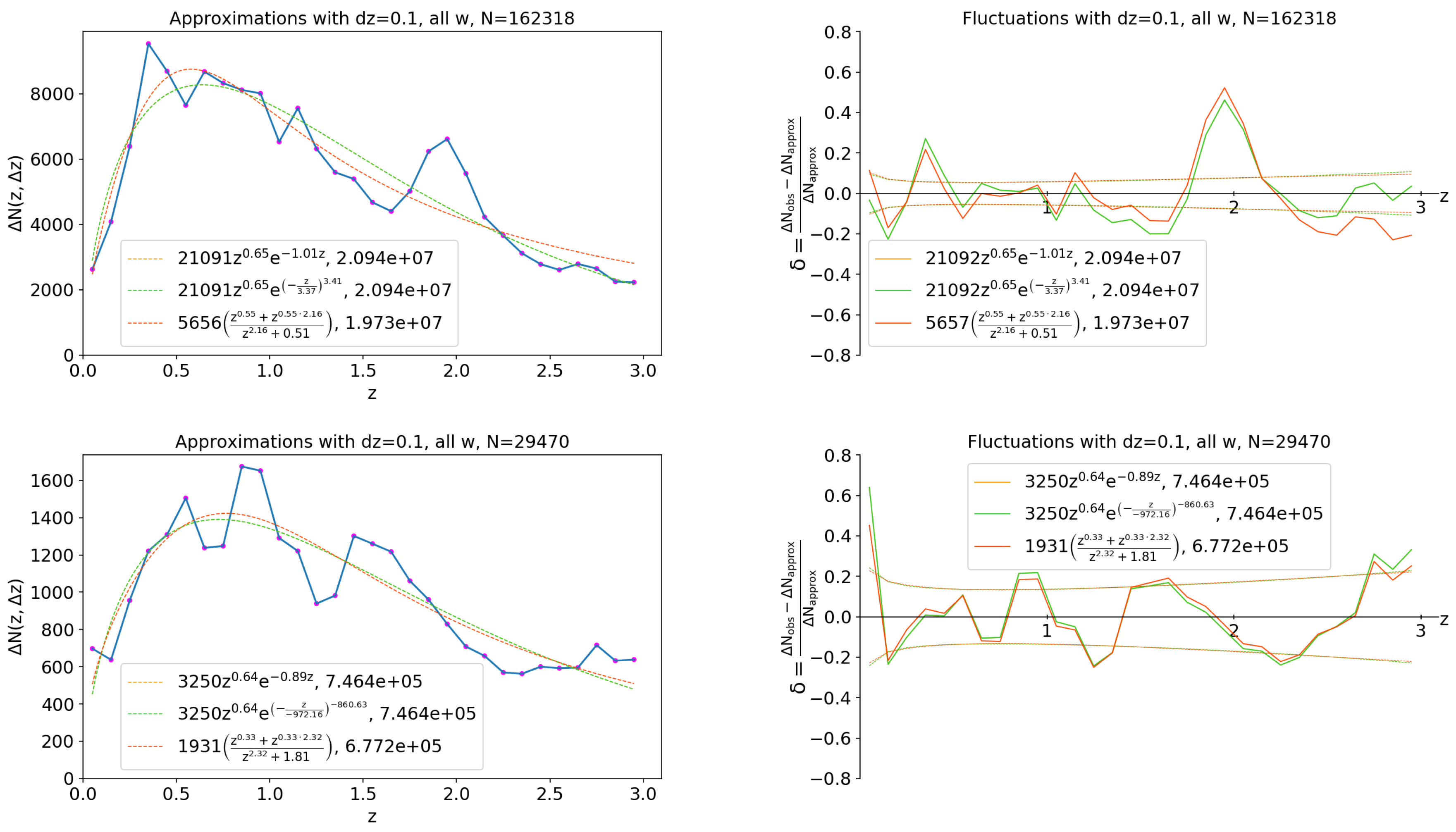
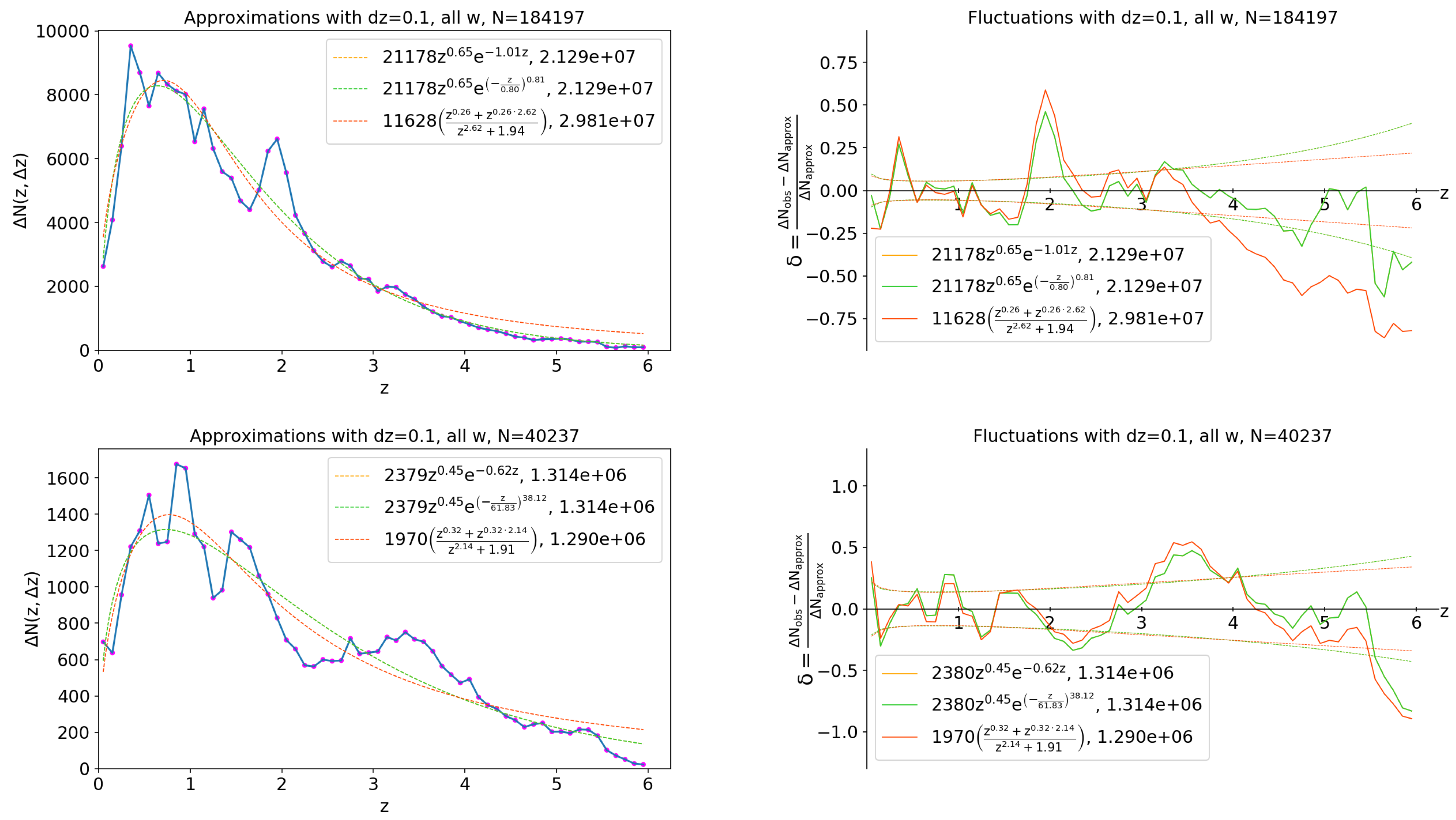
Figure A2. The dotted lines in the fluctuation patterns (right) show the Poisson noise of level 5
. As can be seen in the figures, the COSMOS sample shows four distinct (exceeding the level of
) structures with redshifts:
(void),
(cluster),
(void), and
(cluster). The UltraVISTA sample gives a somewhat different picture, although there is a positive correlation with the COSMOS sample at
, and shows distinct structures at
(void) and at
(cluster).
This result can be explained by the fact that in infrared observations the dust attenuation effects are smaller than in the optical range. Thus, according to the COSMOS2015 catalog data, it can be concluded that optical observations provide rich statistics, and therefore, are useful for the LSSU analysis at redshifts , while infrared observations have a better quality of statistics (in the sense of redshifts) up to .
The structure tables corresponding to
Figure A1 and
Figure A2 are shown in
Table A1 for
, and
Table A2 for
. The parameter
j is the index number of structure, detected by the algorithm. The parameter
n shows the number of bins of a given structure (each structure is a sequence of bins with only positive or only negative fluctuations). The parameter
shows the average redshift value for the bins of each structure, and the errors can be used to restore the centers of the border bins. The parameter
gives an estimate of the metric size of the structure (sequence of bins), where the upper and lower limits correspond to the metric size of the border bins. The parameter
is an estimate of the Poisson noise, which is equal to the ratio of unity to the number of all galaxies in the structure. The parameter
shows level of the observed cosmic variance, where the error is the standard deviation from
within the structure. We also include columns for comparing observations with the predictions of theoretical models. The parameter
shows the theoretical variance of the dark matter density in the
CDM model frameworks. The next column contains the corresponding galaxy bias
, with the errors that are proportional to the errors of the
.
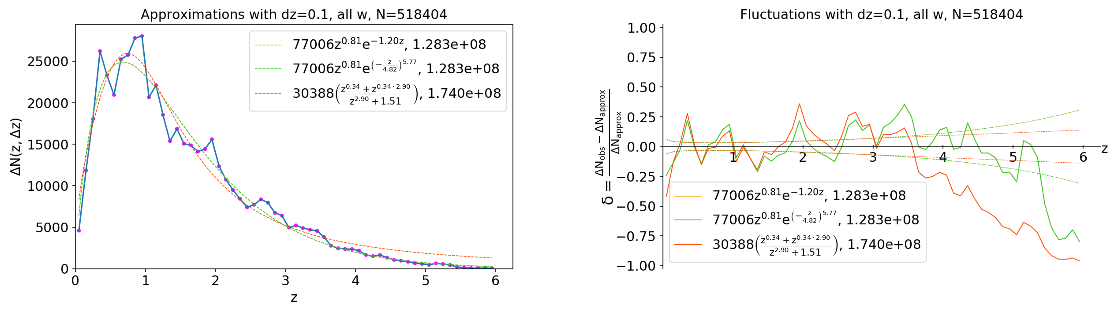
Figure A1.
Histograms of the radial distribution of the COSMOS2015 photometric redshifts and corresponding fluctuation patterns for the disjoint 162,318 COSMOS galaxies (top) and 29,470 UltraVISTA galaxies (bottom) with a bin and without sampling by . The dashed lines indicate the least squares fit (left) and Poisson noise 5 (right).
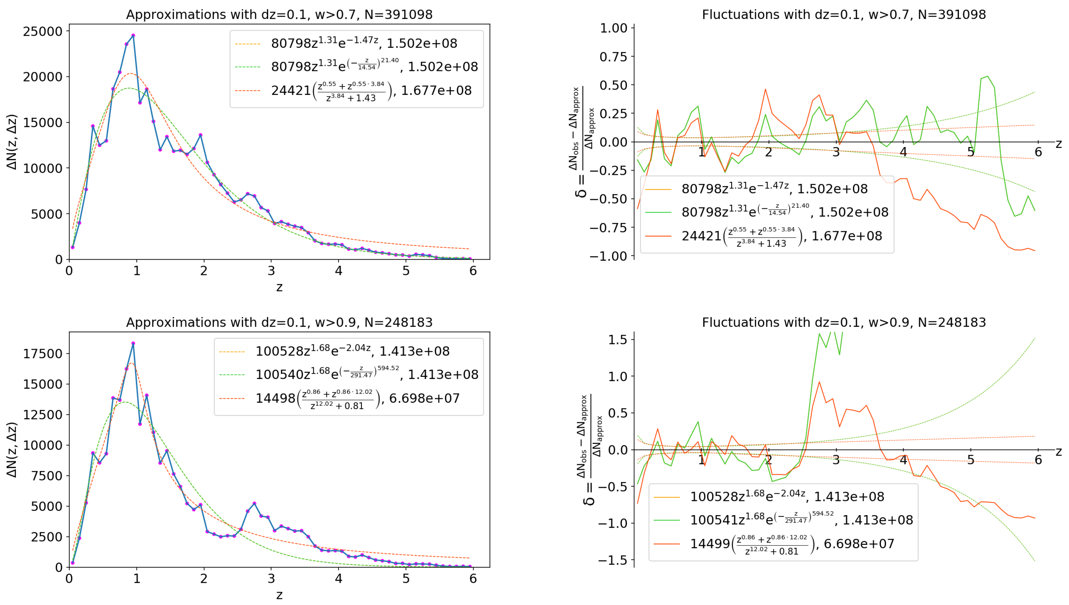
Figure A2.
Histograms of radial distribution of the COSMOS2015 photometric redshifts and the corresponding fluctuation patterns for the disjoint COSMOS galaxies (top) and UltraVISTA galaxies (bottom) with a bin and without sampling by . The dashed lines indicate the least squares fits (left) and Poisson noise 5 (right).
Table A1.
Tables of structures for disjoint the COSMOS (top) and UltraVISTA (bottom) samples from the COSMOS2015 catalogue for a bin
with
and without
selection. The approximation is by empirical Formula (
6). In the last string there are the means of corresponding values (by all structures): mean of redshifts
, mean of structure sizes in Mpc
, mean of Poisson noise level
, mean of observed cosmic variance
, mean of dark matter variance
, mean of dark matter bias
, mean of Peebles correlation function variance
and its bias
(see details in the text).
| Sample | j | n | | , Mpc | | | | | | |
|---|
| Only COSMOS | 1 | 3 | 0.15 ± 0.10 | | 0.008 | 0.100 ± 0.063 | 0.188 | 0.5 ± 0.3 | 0.199 | 0.5 ± 0.3 |
| 2 | 4 | 0.40 ± 0.15 | | 0.006 | 0.063 ± 0.078 | 0.140 | 0.5 ± 0.6 | 0.198 | 0.3 ± 0.4 |
| w = all | 3 | 4 | 0.80 ± 0.15 | | 0.006 | 0.025 ± 0.009 | 0.094 | 0.3 ± 0.1 | 0.178 | 0.1± 0.1 |
| | 4 | 3 | 1.05 ± 0.10 | | 0.007 | 0.020 ± 0.057 | 0.070 | 0.3 ± 0.8 | 0.151 | 0.1 ± 0.4 |
| | 5 | 7 | 1.45 ± 0.30 | | 0.005 | 0.105 ± 0.034 | 0.073 | 1.4 ± 0.5 | 0.184 | 0.6± 0.2 |
| | 6 | 6 | 2.00 ± 0.25 | | 0.006 | 0.185 ± 0.081 | 0.056 | 3.3 ± 1.4 | 0.168 | 1.1 ± 0.5 |
| | 7 | 5 | 2.45 ± 0.20 | | 0.008 | 0.058 ± 0.030 | 0.046 | 1.3 ± 0.6 | 0.154 | 0.4 ± 0.2 |
| | 8 | 3 | 2.75 ± 0.10 | | 0.011 | 0.014 ± 0.026 | 0.035 | 0.3 ± 0.4 | 0.125 | 0.1 ± 0.1 |
| means: | | | 1.38 ± 0.17 | | 0.007 | 0.071 ± 0.021 | 0.088 | 1.0 ± 0.4 | 0.170 | 0.4 ± 0.1 |
| Only UltraVISTA | 1 | 2 | 0.10 ± 0.05 | | 0.028 | 0.202 ± 0.438 | 0.157 | 1.3 ± 2.8 | 0.155 | 1.3 ± 2.8 |
| 2 | 3 | 0.25 ± 0.10 | | 0.018 | 0.109 ± 0.071 | 0.155 | 0.7 ± 0.5 | 0.187 | 0.6 ± 0.4 |
| w = all | 3 | 4 | 0.50 ± 0.15 | | 0.014 | 0.004 ± 0.044 | 0.124 | 0.0 ± 0.0 | 0.192 | 0.0 ± 0.0 |
| | 4 | 4 | 0.90 ± 0.15 | | 0.014 | 0.077 ± 0.082 | 0.087 | 0.9 ± 0.9 | 0.174 | 0.4 ± 0.5 |
| | 5 | 5 | 1.25 ± 0.20 | | 0.013 | 0.071 ± 0.066 | 0.075 | 0.9 ± 0.9 | 0.176 | 0.4 ± 0.4 |
| | 6 | 5 | 1.65 ± 0.20 | | 0.014 | 0.111 ± 0.028 | 0.062 | 1.8 ± 0.4 | 0.167 | 0.7 ± 0.2 |
| | 7 | 9 | 2.25 ± 0.40 | | 0.012 | 0.104 ± 0.031 | 0.055 | 1.9 ± 0.6 | 0.175 | 0.6 ± 0.2 |
| means: | | | 0.99 ± 0.18 | | 0.016 | 0.097 ± 0.023 | 0.102 | 1.2 ± 0.3 | 0.175 | 0.7 ± 0.2 |
Table A2.
Tables of structures for disjoint the COSMOS (top) and UltraVISTA (bottom) samples from the COSMOS2015 catalogue for a bin
with
and without
selection. The approximation is by empirical Formula (
6). In the last string there are the means of corresponding values (by all structures): mean of redshifts
, mean of structure sizes in Mpc
, mean of Poisson noise level
, mean of observed cosmic variance
, mean of dark matter variance
, mean of dark matter bias
, mean of Peebles correlation function variance
and its bias
(see details in the text).
| Sample | j | n | | , Mpc | | | | | | |
|---|
| Only COSMOS | 1 | 3 | 0.15 ± 0.10 | | 0.008 | 0.098 ± 0.064 | 0.188 | 0.5 ± 0.3 | 0.199 | 0.5 ± 0.3 |
| 2 | 4 | 0.40 ± 0.15 | | 0.006 | 0.063 ± 0.078 | 0.140 | 0.5 ± 0.6 | 0.198 | 0.3 ± 0.4 |
| w = all | 3 | 4 | 0.80 ± 0.15 | | 0.006 | 0.024 ± 0.009 | 0.094 | 0.3 ± 0.1 | 0.178 | 0.1 ± 0.1 |
| | 4 | 3 | 1.05 ± 0.10 | | 0.007 | 0.021 ± 0.057 | 0.070 | 0.3 ± 0.8 | 0.151 | 0.1 ± 0.4 |
| | 5 | 7 | 1.45 ± 0.30 | | 0.005 | 0.106 ± 0.034 | 0.073 | 1.5 ± 0.5 | 0.184 | 0.6± 0.2 |
| | 6 | 6 | 2.00 ± 0.25 | | 0.006 | 0.185 ± 0.081 | 0.056 | 3.3 ± 1.4 | 0.168 | 1.1 ± 0.5 |
| | 7 | 5 | 2.45 ± 0.20 | | 0.008 | 0.058 ± 0.030 | 0.046 | 1.2 ± 0.6 | 0.154 | 0.4 ± 0.2 |
| | 8 | 3 | 2.75 ± 0.10 | | 0.012 | 0.016 ± 0.025 | 0.035 | 0.3 ± 0.5 | 0.125 | 0.1 ± 0.1 |
| | 9 | 7 | 3.35 ± 0.30 | | 0.010 | 0.066 ± 0.032 | 0.039 | 1.7 ± 0.8 | 0.155 | 0.4 ± 0.2 |
| | 10 | 3 | 3.75 ± 0.10 | | 0.017 | 0.014 ± 0.015 | 0.028 | 0.0 ± 0.0 | 0.118 | 0.0 ± 0.0 |
| | 11 | 13 | 4.45 ± 0.60 | | 0.011 | 0.128 ± 0.028 | 0.034 | 3.7 ± 0.8 | 0.159 | 0.8 ± 0.2 |
| | 12 | 3 | 5.25 ± 0.10 | | 0.033 | 0.041 ± 0.036 | 0.022 | 1.2 ± 1.0 | 0.112 | 0.2 ± 0.2 |
| means: | | | 2.32 ± 0.20 | | 0.011 | 0.068 ± 0.015 | 0.069 | 1.3 ± 0.4 | 0.158 | 0.4 ± 0.1 |
| Only UltraVISTA | 1 | 3 | 0.25 ± 0.10 | | 0.018 | 0.132 ± 0.095 | 0.155 | 0.9 ± 0.6 | 0.187 | 0.7 ± 0.5 |
| 2 | 4 | 0.50 ± 0.15 | | 0.014 | 0.045 ± 0.045 | 0.124 | 0.3 ± 0.4 | 0.192 | 0.2 ± 0.2 |
| w = all | 3 | 4 | 0.90 ± 0.15 | | 0.014 | 0.130 ± 0.087 | 0.087 | 1.5 ± 1.0 | 0.174 | 0.7 ± 0.5 |
| | 4 | 5 | 1.25 ± 0.20 | | 0.013 | 0.056 ± 0.065 | 0.075 | 0.7 ± 0.8 | 0.176 | 0.3 ± 0.4 |
| | 5 | 4 | 1.60 ± 0.15 | | 0.015 | 0.101 ± 0.028 | 0.059 | 1.7 ± 0.5 | 0.158 | 0.6 ± 0.2 |
| | 6 | 11 | 2.25 ± 0.50 | | 0.010 | 0.175 ± 0.039 | 0.057 | 3.1 ± 0.7 | 0.179 | 1.0 ± 0.2 |
| | 7 | 3 | 2.85 ± 0.10 | | 0.022 | 0.002 ± 0.023 | 0.035 | 0.0 ± 0.0 | 0.124 | 0.0 ± 0.0 |
| | 8 | 15 | 3.65 ± 0.70 | | 0.012 | 0.249 ± 0.041 | 0.040 | 6.2 ± 1.0 | 0.166 | 1.5 ± 0.3 |
| | 9 | 6 | 4.60 ± 0.25 | | 0.024 | 0.043 ± 0.029 | 0.030 | 1.2 ± 0.8 | 0.143 | 0.3 ± 0.2 |
| | 10 | 4 | 5.00 ± 0.15 | | 0.033 | 0.061 ± 0.032 | 0.025 | 2.0 ± 1.0 | 0.127 | 0.4 ± 0.2 |
| | 11 | 4 | 5.30 ± 0.15 | | 0.036 | 0.044 ± 0.045 | 0.024 | 1.0 ± 1.1 | 0.126 | 0.2 ± 0.2 |
| means: | | | 2.56 ± 0.24 | | 0.019 | 0.094 ± 0.023 | 0.065 | 1.9 ± 0.5 | 0.159 | 0.6 ± 0.1 |
The next column contains the approximation of the matter density
, distributed according to the PLCF with the parameters
(see Tables 3 and 4 in Shirokov et al. [
9]). At high redshifts (
), linear extrapolation of the data in logarithmic coordinates was used to determine
. Column
contains the corresponding bias parameter, where errors are calculated in the same ways as
. The bias value
indicates that the Poisson noise is higher than
, and this structure is excluded from the
function, as well as from the calculation of the average bias value
.
Last row contains the following average values of corresponding parameters over all structures detected in a sample of galaxies: average redshift
, average size of structures in Mpc
, average Poisson noise level
, average observed cosmic variance
, average dark matter variance
, average dark matter bias
, average Peebles correlation function variance
and its bias
. Errors of all the target values correspond to the standard deviation of the corresponding parameters for all structures, except for
, which is calculated by the Formula (
12).
The catalogue contains an interesting note about redshift columns: “a comparison photo-z/spec-z shows that these errors could be underestimated by a factor 0.1 * I – 0.8 at I > 20 and 1.2 at I < 20”. Taking this into account one can improve the picture of spatial structures of the catalog and enhance the correlation of density fluctuations between independent surveys of this field in future studies.

 ,
, 


