Article

Predicting >10 MeV SEP Events from Solar Flare and Radio Burst Data

Department of Languages and Computer Sciences, Universidad de Málaga, 29016 Málaga, Spain
*
Author to whom correspondence should be addressed.
Universe 2020, 6(10), 161; https://doi.org/10.3390/universe6100161
Submission received: 23 August 2020 / Revised: 24 September 2020 / Accepted: 25 September 2020 / Published: 28 September 2020
(This article belongs to the Section Solar System)

Abstract

:
The prediction of solar energetic particle (SEP) events or solar radiation storms is one of the most important problems in the space weather field. These events may have adverse effects on technology infrastructures and humans in space; they may also irradiate passengers and flight crews in commercial aircraft flying at polar latitudes. This paper explores the use of ≥ M2 solar flares and radio burst observations as proxies for predicting >10 MeV SEP events on Earth. These observations are manifestations of the parent event at the sun associated with the SEP event. As a consequence of processing data at the beginning of the physical process that leads to the radiation storm, the model may provide its predictions with large anticipation. The main advantage of the present approach is that the model analyzes solar data that are updated every 30 min and, as such, it may be operational; however, a disadvantage is that those SEP events associated with strong well-connected flares cannot be predicted. For the period from November 1997 to February 2014, we obtained a probability of detection of 70.2%, a false alarm ratio of 40.2%, and an average anticipation time of 9 h 52 min. In this study, the prediction model was built using decision trees, an interpretable machine learning technique. This approach leads to outputs and results comparable to those derived by the Empirical model for Solar Proton Event Real Time Alert (ESPERTA) model. The obtained decision tree shows that the best criteria to differentiate pre-SEP scenarios and non-pre-SEP scenarios are the peak and integrated flux for soft X-ray flares and the radio type III bursts.

Graphical Abstract

1. Introduction

Solar energetic particle (SEP) events are produced when particles emitted by the Sun are accelerated during a flare or by coronal mass ejection (CME)-driven shocks [1] and reach the Earth along interplanetary magnetic field lines. The associated solar eruptions on the Sun are observed at several wavelengths, including soft X-rays, extreme ultraviolet (EUV), and radio. Energetic protons and ions are the main constituents of SEP events, and their effects are more severe than other particles, such as electrons. In space, SEP events may pose a significantly high risk of cancer to astronauts and damage a spacecraft’s electronic components [2,3,4,5]. On Earth, SEPs may irradiate passengers and flight crews in aircraft flying at polar latitudes [6,7,8].
In this paper, SEP events refer to the detection of high fluxes of energetic protons and ions in the near-Earth environment. Forecasting SEP events helps to improve mitigation of the aforementioned adverse effects. The prediction of SEP events is a challenge not only because these events are complex physical processes, the physics of which is still under study, but also because they are rare events. Indeed, in the period 2007–2020, only 42 SEP events were detected by the Geostationary Operational Environmental Satellite (GOES) satellites (J (E > 10 MeV) >10 proton flux units (pfu)).
The objective of this work is to predict the occurrence of SEP events with energies >10 MeV from flare and radio burst data. This study explores the use of an interpretable machine learning technique to predict >10 MeV SEP events from National Oceanic and Atmospheric Administration/Space Weather Prediction Center (NOAA/SWPC) data files, which may be easily obtained online. The final purpose of the model, called the University of Malaga predictor from Solar Data (UMASOD), is to optimize the probability of detection (POD), false alarm ratio (FAR), and average warning time (AWT). The first two metrics are optimized by maximizing the critical success index (CSI), which is used in atmospheric meteorology to assess severe weather predictors, providing a way to combine POD and FAR in a single value. Regarding the anticipation time (i.e., AWT), we approach it using flare data and radio burst data which are observational data at the beginning of the physical process.
Other approaches have also been proposed to analyze solar flare and radio data to predict the occurrence of >10 MeV SEP events [9,10,11]. In this paper, we call these approaches radio-data-based SEP event predictors. We compare our forecasting results with those obtained by the Empirical model for Solar Proton Event Real Time Alert (ESPERTA) model [10,11], which is the cutting edge in radio-data-based SEP event predictors. Currently, ESPERTA is not in operation because the radio data on which it depends are not available in real time.
Machine learning is a set of techniques for discovering knowledge and correlations from data with several purposes. These techniques have been used for the identification of patterns in datasets, employing several different tasks such as classification, regression, and summarization, among others. In the field of SEP event predictions, several machine learning techniques have been used. For example, Winter and Ledbetter [1] employed principal component analysis (PCA) to show that solar flare and radio burst data can lead to effective >10 MeV SEP prognosis. Boubrahimi et al. [12] used interpretable decision tree (DT) models for predicting >100 MeV SEP events from solar soft X-ray (SXR) and in situ proton observations. In this study, we also use interpretable DT models for predicting >10 MeV SEP events from solar flare and radio burst data.
This paper is organized as follows: Section 2 describes the problem to solve, including a brief explanation about solar proton events, flares, and radio bursts. Section 3 describes our approach to constructing the prediction model. Section 4 discusses the results and compares them with those obtained by other similar approaches, and Section 5 presents the conclusions.

2. Description of the Problem
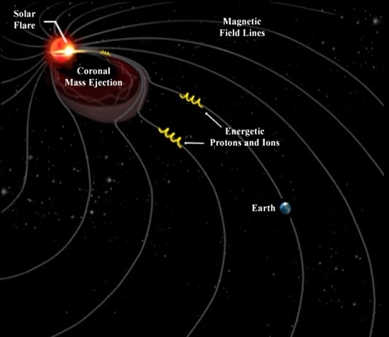
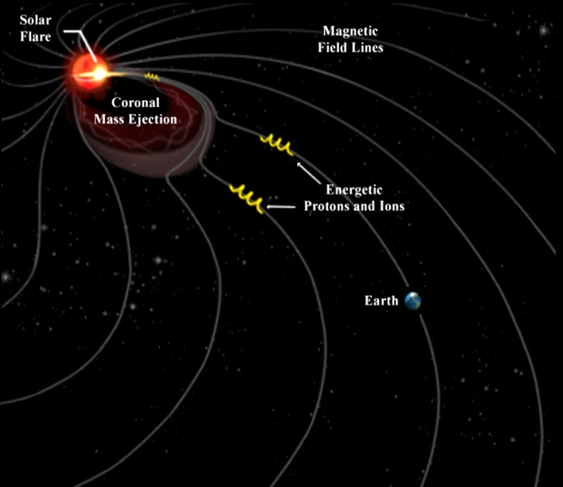
During a strong solar eruption, a flare and a CME take place. Solar eruptions are monitored using soft X-rays and radio data. A solar eruption may lead (with a low probability) to the occurrence of solar radiation storm in the near-Earth environment.
In this section, we present a brief description of these phenomena and the relation between them.

2.1. SEP Events

It is known that the frequency of SEP events varies, following a periodic 11year cycle of solar activity. In Figure 1, the evolution of the number of sunspots is shown, and the solar cycles can be clearly observed. It is important to learn prediction knowledge from a variety of solar and interplanetary situations; for this reason, in this study we used events from 1997 to 2014, which covered the entire 23rd solar cycle and part of the 24th cycle.
SEPs are accompanied by other phenomena like flares and radio bursts, which are discussed below.

2.2. Solar Flares

A solar flare is a sudden brightening in the solar atmosphere, typically spread across all atmospheric layers and involving substantial mass motions and particle acceleration. A solar flare occurs when magnetic energy in the solar atmosphere is suddenly released.
Solar flares can be described using various parameters such as heliolongitude and heliolatitude, brightness, area, and X-ray flux. Solar flares are classified into five classes (A, B, C, M, X), according to the peak flux of the soft X-rays, with the X-class flares being the most intense ones. Within each class, a number is put to indicate the intensity (e.g., an M1 flare is less intense than an M2 flare). Like ESPERTA [10,11], our model is triggered by ≥M2 flares to predict >10 MeV SEP events.

2.3. Radio Bursts

The research on solar radio bursts provides considerable possibilities for the study of some important pre-phenomena in solar physics. It is important to separate fixed-frequency radio bursts and sweep-frequency radio bursts. The first analysis type only considers some discrete frequencies and measures the peak values of microwaves at these frequencies; moreover, they were used before to predict SEPs with good results [13]. Regarding the shape of the radio burst, some different types of sweep-frequency radio bursts can be distinguished.
Although there is a larger number of solar radio burst types, types II to IV are briefly introduced below as they are known to be related to pre-SEP scenarios.
  • Type II:
These bursts are indications of the shock acceleration of electrons. They typically occur at around the time of the SXR flux peak in a solar flare, when the CME has already erupted and there is a shock. They drift slowly in frequency and last between a few minutes and half an hour, with a frequency range of approximately 50 to 120 MHz [13,14,15,16,17].
  • Type III:
Type III bursts are produced by electron beams traveling outward throughout the corona and interplanetary space. They are brief radio bursts that drift very rapidly in frequency versus time. They occur over a frequency range of 10 kHz to 8GHz and are associated with flares, although not every flare is accompanied by a type III burst. Although not as frequent, type III bursts may also travel inward, toward the solar surface [14,15,16,17,18,19].
  • Type IV:
The broadband and non-drifting nature of type IV emission has led to the widespread belief that they are due to trapped electrons in closed magnetic structures, which could be low in the corona during flares, or trapped electrons in a CME directed toward Earth. They are indications that very energetic electrons are forced to turn and, thus, have not escaped, but there is an intense electron activity. Type IV bursts are broadband quasi-continuum features associated with the decay phase of solar flares. These radio bursts are also nearly always associated with large flares of long duration. There are also drifting cases which could indicate that electrons escape. Type IV bursts are also associated with type II bursts [13,15,16,17].
Current association between SEPs and radio bursts:
Solar radio bursts were connected in past studies to energetic particles in general and SEP events in particular [5,8,15,16,17,18,19,20,21,22,23]. In brief, the currently accepted role of radio bursts in SEP predictions may be summarized as follows: there is a high association between SEP events and type III bursts (electron escape) during the first phase of solar eruptions, followed by type II (shock-accelerated electrons in the interplanetary medium) and IV (trapped electrons in a magnetic structure, e.g., a traveling CME).
It is important to mention that the radio emissions are only due to electrons. However, like ESPERTA, our model associates remote SXR and radio signatures with in situ protons, despite the fact that there is no direct cause–effect association. A current empirical association [21,24] is that if there is evidence that electrons were accelerated and could escape, then it is also probable that protons could also be accelerated and escape.
Table 1 shows a compilation of the characteristics and associated phenomena of these bursts. Moreover, the information about the NOAA edited event files [25] describes the remaining bursts types (V, VI, VII, and broadband long-lived dekametric continuum (CTM)) which are not explained here because, in Section 4, they were found to be irrelevant for predicting SEP events.

3. Methodology

The purpose of the proposed UMASOD model is to process the NOAA/SWPC Solar Edited Event file to build a decision tree that predicts >10 MeV SEP events. In order to obtain the training examples, we took two data sources. We used the SWPC Solar Event list [25] provided by the NOAA to build the unlabeled training examples; then, each of these examples were labeled with either “an SEP event is expected” or “no SEP event is expected” using the SEP list [26] provided by NASA and NOAA with the SEPs detected on Earth. During real-time operations, the final model should be able to use the analysis of the NOAA/SWPC Solar Edited Event file to predict >10 MeV SEP events. These files are updated every 30 min at 2 and 32 min past the hour.
The first data source, i.e., the NOAA/SWPC Solar Edited Event files, includes all the information about a great number of solar phenomena such as flares, CMEs, and radio bursts. Each file includes specific information about each type of phenomenon and a solar eruption code. Our pre-processing program gets the information on radio bursts, flares, and X-Rays, and saves it in an event list, called here the “Solar Event List”, which is used as the training dataset. An SEP event is associated with a single solar eruption code. A solar eruption is a complex process that is associated with several solar events (e.g., a flare, a radio burst); for this reason, several solar events may share the same (solar eruption) code.
The second source, the NOAA/NASA SEP list, is used only during the training phase. This list provides information about the intensity of SEP events, as well as information about the associated solar flare.
Both sources, the SWPC event list and the SEP list, provide flare time, peak, and location data, which are used to associate the data in both lists. Thus, for the period 1997–2014, our pre-processing program successfully associated 96 of the 98 SEPs (with full information) with an event from the event list. The information on the SEPs was added to the related solar events, and then filtered, taking into account only the events with a flare peak ≥M2, i.e., the filtering criterion used by the ESPERTA model [10,11]. The obtained event list contained a high proportion of negative instances.

3.1. Pre-Processing Events from NOAA/NASA Files

The first step in this study consisted of reading all the information provided in the NOAA files. Two different types of files were used.
Firstly, the NOAA edited event list [25] includes all the information related to flares, X-rays, coronal mass ejections, and radio bursts. Since 1997, this event list file has been edited daily and information is updated every 30 min. The file specifies the following information for each of these phenomena:
  • An event ID, which identifies the different phenomena that are associated with the same event, as well as the beginning and end of the phenomenon. It also includes the peak time for some of them.
  • The observatory that measured the phenomena, from a list of seven observatories in the USA, Australia, and Italy. The quality of the measurements is also presented.
  • The type of phenomenon, which includes all the phenomena previously cited, and others that are not relevant for this work. There is also specific information, depending on the type. This is explained later.
  • The assigned solar region number.
Our pre-processing program recorded a total of 89,002 different events from 1997 to 2014.
Secondly, the NOAA/NASA SEP list [26] includes all the information on SEP events since 1976. The following data are shown for every SEP event:
  • Start and peak time of the event, and maximum proton flux.
  • Associated CME, only since 1997.
  • Associated flare, including the time when the peak of the flare was produced, the importance of the flare, the location in heliolatitude and heliolongitude, and the region.
The program recorded a total of 98 SEP events from 1997 to February 2014.
Firstly, our pre-processing program read the edited event list files from 1997 to 2014. The data were stored in our Solar Event List, which contained the following properties:
  • ID of the event,
  • Date of the event,
  • Peak value of the flare taken from X-ray information, if it exists,
  • Start, end, and peak times, also taken from X-ray information,
  • The location of the flare in solar coordinates,
  • Intensity, frequency range, duration, and rise time for each of the different types of sweep-frequency radio bursts included in the edited event list. The frequency range of the radio sweep bursts was 25–180 MHz.
Secondly, the program read the mentioned NOAA/NASA SEP list file. The program recorded the information of all the SEPs from 1997 to February 2014 in another list, called here the “Storm List”, which contained all the fields mentioned above except for the associated CME and the region of the flare. There were a total of 125 SEPs during this period, but only 98 of them had information in all the fields.

3.2. Associating Events

Events from both lists (i.e., the Solar Event List and the Storm List) were associated. The procedure was as follows. Firstly, for each SEP in the Storm List, the program checked if it had information in all fields. If so, the program searched the Solar Event List for those events that happened within the prior 24 h of the occurrence of the SEP event. Then, from those events, the peak value of the flare was compared with the peak value of the associated flare of the SEP event. If there was more than one event with the same peak within the prior 24 h, the program looked for the coordinates of the flare and took the closer one to the associated flare coordinates.
After this process, 96 of the 98 SEP events mentioned above were successfully related to items in the Solar Event List. The two remaining SEPs were the event of 4 November 2003, because there was no event with the same peak value that day, and the event of 6 January 2014, because there was no event file from the NOAA for that day. Both events were excluded.
The information from the Storm List was saved into the associated events in the Solar Event List, and a Boolean property in the solar event was changed to the true class (i.e., “an SEP event is expected”), indicating that it produced an SEP event; otherwise, the solar event was labeled with the false class (i.e., “no SEP event is expected”).

3.3. Filtering Events

The next step involved filtering both positive events, i.e., those with an associated SEP, and negative events, mainly according to their X-ray peak.
These filters were applied in two steps. In the first place, all events that contained neither an SEP event nor a sweep-frequency radio burst (I–VII) were discarded. The remaining events were filtered as a function of their X-ray peak, discarding all events below M2. Since the M2 threshold worked properly for the ESPERTA model [10,11], we used it in our approach.
After this process, only 75 out of 96 SEP events passed the filter. However, the Solar Event List went from the previously mentioned 89,002 events to only 502. This means that there were 75 positive instances, i.e., solar events whose class was true (i.e., an SEP took place after the event was observed on the Sun), and 427 negative ones. Table 2 shows a compilation of all SEP events that passed the filter.

3.4. Usability of the Radio Burst Information

Up to now, the obtained events list contains the information of the seven sweep-frequency radio burst types, but it is possible that part of this information cannot be used for predicting an SEP event.
In general, a real-time SEP occurrence prediction model should issue the predictions before the start time of the SEP events (e.g., the time at which the >10 MeV integral proton flux surpasses 10 pfu). Therefore, such models have to be trained only with information that is available before the start time of the SEP events. That is, any datum that is not available before the SEP event start time is not useful for real-time prediction purposes; thus, it should be discarded from the training and testing phases. For example, if a radio burst ends after the start time of the SEP event, it is not possible to use the information of the radio burst to predict the SEP. Therefore, to know which radio bursts are useful for making real-time SEP occurrence predictions, the pre-processing program generates a table that contains, for each SEP event, the lists of differences in minutes between the end time of each type of sweep-frequency radio burst (RSP) and the SEP start time. This information is shown in Table 3. Since a single event does not contain all types of radio bursts, the table shows a “-” if the event does not contain that particular type. We must note that the event of 24 August 1998 contained an anomalous date for the radio burst types II and IV, and these radio bursts took place before the SEPs.
As can be seen in Table 4, the end of the sweep-frequency radio bursts of type IV is very likely to take place after the start of the SEP event, and type V is related to a low percentage of SEP events. Because of that, these types of radio bursts were excluded hereinafter from the generation of the model.
Table 4 shows the number of radio bursts that ended before the start of the SEP event in relation to the number of radio bursts of each type.

3.5. Preparing Instances for the Machine Learning

Before starting the generation of the prediction model, it was necessary to calculate some new variables as a combination of others or to discretize some continuous attributes.
Firstly, the program discretized the location of the flare of the event; to be able to do this, it was necessary to obtain the heliolongitude and heliolatitude from the location string of the form “N30W40”. The heliolatitude takes an integer value from −90 (S90 i.e., south 90) to +90 (N90 i.e., north 90), while the heliolongitude can take values below 90 (W90 i.e., west 90) and over −90 (E90 i.e., east 90), if the flare is produced on the back side of the Sun. Then, the program saved a discretization of these values in the variables Discrete Heliolongitude, and Discrete Heliolatitude, dividing each coordinate into 12 regions.
Secondly, the SXR peak was saved as the logarithm of the soft X-ray peak flux with flare classes of C, M, and X, meaning 10−6, 10−5, and 10−4 Watts/m2, respectively; for example, a value of X2.5 means an SXR flux of 2.5 × 10⁻⁴ Watts/m2. In this way, the classes followed a linear progression instead of an exponential progression. The program also discretized the logarithm value, dividing the scale into 22 sections, and saving it if the logarithm was greater than each one of the 21 points of divisions (e.g., SXR ≥ X2.5). This information was stored in a Boolean array.
Thirdly, the program also calculated the duration and rise time, in minutes, of the flare and each of the radio bursts, saving this information in the events.
Lastly, the program calculated the approximate integrals of each of the sweep-frequency radio burst fluxes for each event. To calculate these approximate integrals, it simply multiplied the intensity of the radio burst and the duration of the phenomenon in minutes. This information was stored inside the event. Then, following the example of Laurenza [10], who multiplied the integral of X-rays and the integral of microwave to predict the occurrence of SEP events, the program calculated the product of the integral of X-rays and radio bursts of types II and III, which were the most common radio types. It was necessary to calculate 10 thresholds for each type. These thresholds were the percentiles 0, 10, 20, etc. of the products of the integral of each event with a related SEP event. The program stored, in two Boolean arrays, whether the products of the integrals of X-ray and radio bursts of types II and III exceeded their respective thresholds.
All this information, together with the previous data from NOAA/NASA files, was exported to a CSV file containing the values of the attributes of the 502 events mentioned, as well as a Boolean class, which was true if there was an SEP event and false otherwise.

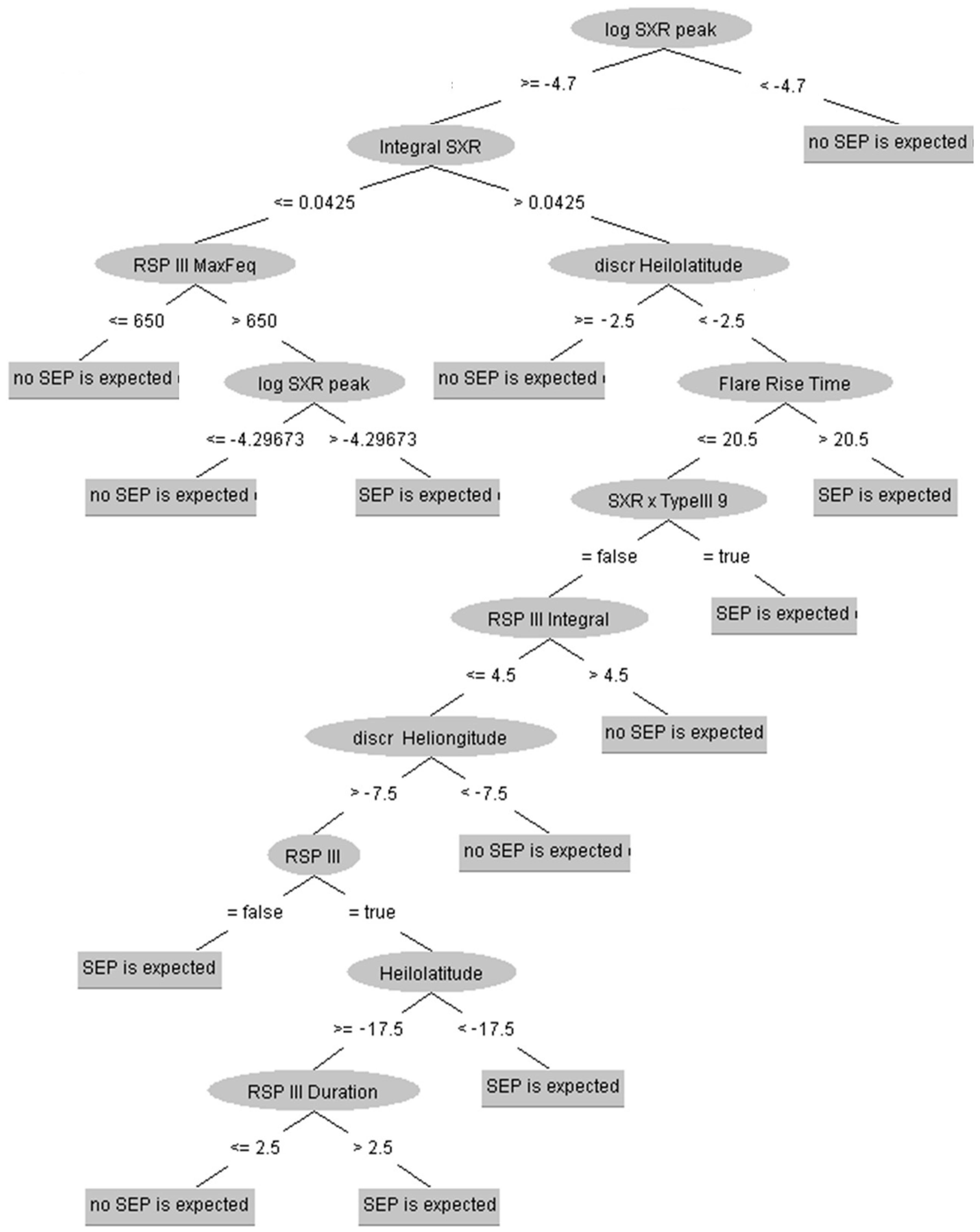
3.6. Generating the Prediction Model

As explained above, the class was imbalanced, with 75 positive events and 427 negative ones, i.e., a 15%/85% proportion. Training datasets with imbalanced class distribution are an important problem in machine learning [27]. The main approaches to this issue are sampling methods, cost-sensitive methods, and instance-weighting methods.
The first involves the modification of the dataset via various mechanisms to provide a balanced distribution [28]. This can be made via oversampling, i.e., adding copies of the minority class, or under-sampling, i.e., removing copies of the majority class.
The second considers the costs associated with misclassifying examples and applies a different cost from cost matrices to each data example as a function of its class value [29].
The third weights the instances in the data such that each class has the same total weight, maintaining the total sum of weights across all instances [30].
These three methods were compared and there was no clear winner [31] among them regarding performance. This paper used the instance-weighting approach implemented in Weka via the ClassBalancer Filter [32].
For the generation of the decision tree, the J48 algorithm was used [33]. We developed a program that uses the Weka API [34] to try different values of the minimum number of instances per leaf to generate the model, evaluating them by 20-fold cross-validation. With the minimum number of instances per leaf, the program generates a model and evaluates it by cross-validation, thereby optimizing the POD and FAR of the model. We carried out the optimization approach described in Section 3.7.
The errors obtained here were errors of generalization, i.e., the error calculated using a testing set whose examples were not included in the training set. POD and FAR are two frequently used metrics in the prediction of SEP events. POD is the number of SEPs correctly classified compared to the total number of SEP events occurred. FAR is the number of false alarms compared to the number of false alarms plus the number of SEPs correctly classified.

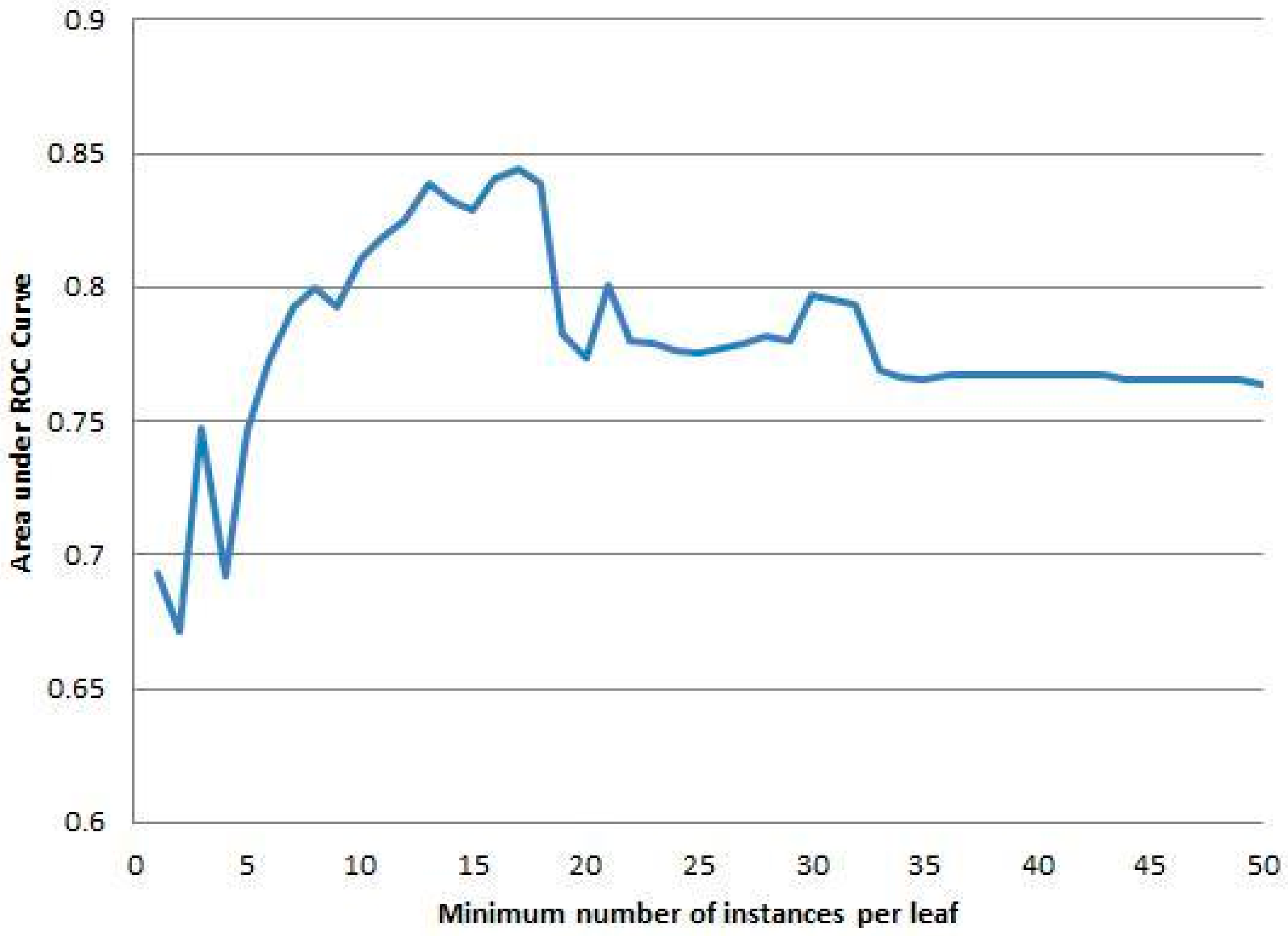
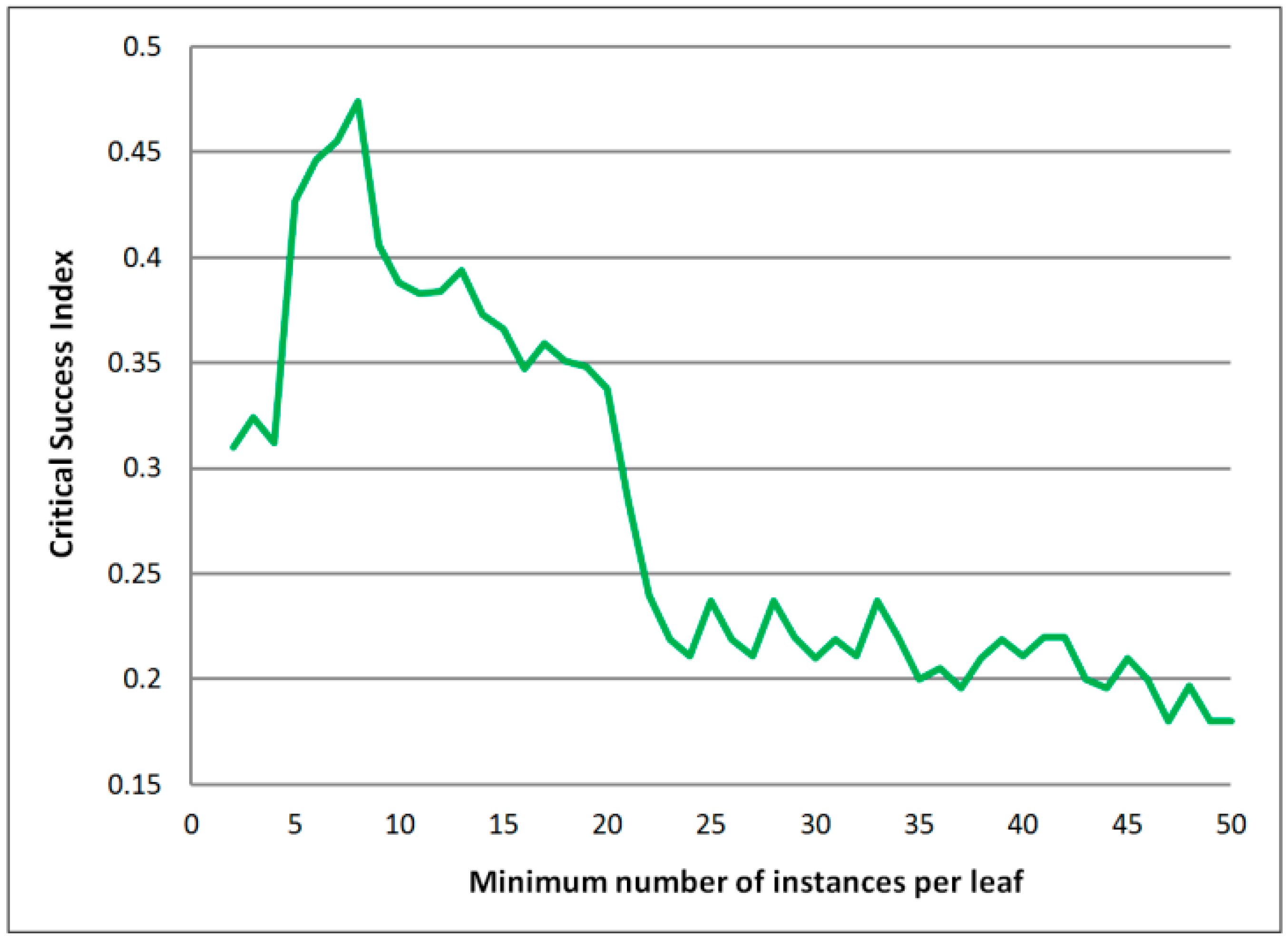
3.7. Optimization of the Decision Tree

Usually, there are two event-oriented prediction performance metrics that can be used for the optimization of the decision tree: receiver operating characteristic [35] area under the curve (ROC-AUC) and precision recall area under the curve (PR-AUC) [36]. There is an additional event-oriented prediction performance metric, mostly used by atmospheric weather experts, called the critical success index (CSI) [37], which can also be applied for optimization purposes.
Regarding the ROC-AUC approach, an ROC curve is the plot of the true positive rate (TPR) against the false positive rate (FPR). The TPR is defined as TPR = TP/(TP + FN), and the FPR is defined as FPR = FP/(FP + TN), where TP = true positive, TN = true negative, FP = false positive, and FN = false negative. The goal of the ROC-AUC is to have the model be at the upper left corner. A higher area under the ROC curve denotes a better model. In order to use this approach, we used a 20-fold cross-validation, varying the minimum number of instances per leaf. Figure 2 shows the area under the curve as a function of the minimum number of instances per leaf. As seen, taking into account the ROC-AUC approach, the best number of instances per leak was 17. By using the 20-fold cross-validation on the training and validation sets of solar events (i.e., associated with ≥M2 flares) and the ROC-AUC optimization approach, the obtained POD was 80% (60/75) and the FAR was 61.54% (96/156).
When being confronted with the class imbalance problem [27,28], the TN count (i.e., true negative) was too large, providing an FPR that was too low in all predictors. For this reason, ROC-AUC analysis [35] did not provide useful comparative results among predictors, which is why the PR-AUC [36] and the CSI approach [37] were used. Regarding the PR-AUC approach, the PR curve plots precision against recall. Precision is defined as TP/(TP+FP), and recall is defined as TP/(TP+FN). Note that recall is POD and precision is 1 − FAR. In the case of the PR-AUC, the goal is to have the model be at the upper right corner, which basically represents only true positives with no false positives and no false negatives. The precision recall area under curve (PR-AUC) is just the area under the PR curve. According to this approach, a higher value denotes a better model. The main difference between the ROC-AUC and PR-AUC is that the PR does not account for true negatives (as TN is not a component of either precision or recall). The PR-AUC approach uses a combination of POD and 1 − FAR. Note that there is no single way to combine POD and FAR.
In this study, we used the CSI to optimize the POD and FAR. CSI is a metric that proved its utility after decades of use by atmospheric weather experts. The US National Weather Service uses this measure to assess predictors because, according to them [37], it is an unbiased verification statistic appropriate for predicting rare events, and, for this reason, it is used to assess severe weather predictors. CSI has also been used in SEP event prediction modeling for optimizing POD and FAR [38,39,40]. The CSI combines POD and FAR as follows: CSI = (POD−1 + (1 − FAR)−1 − 1)−1. An CSI of 100% is the indication of an excellent predictor with POD= 100% and FAR= 0%. In order to optimize our model using CSI, we used a 20-fold cross-validation evaluation over the training and testing cases, varying the minimum number of instances per leaf. For each cross-validation, we obtained the POD and FAR, which were used for calculating the CSI.
Figure 3 presents the CSI index as a function of the minimum number of instances in the leaf. Taking into account the CSI, the best number of instances per leaf was eight. By using the 20-fold cross-validation on training and validation sets of solar events (i.e., associated with ≥M2 flares) and the application of the CSI optimization approach, the obtained POD was 85.3% (64/75) and the FAR was 54.6% (77/141).
Note that the resulting POD using ROC-AU analysis was the same as that using the CSI-based approach, but the FAR was better (54.6% vs. 61.54%) using the CSI-based approach, mainly because it is only driven by the optimization of POD and FAR, and the ROC analysis is not.

3.8. Analysis of Variable in the Decision Tree

The final predictive decision tree (see Figure 4) was constructed using the J48 method with the Weka tool [34] and the optimization approach, explained in Section 3.7. Note that the first node of the tree is actually the filtering of the <M2 flares that we performed, as our model only considered events associated with flares ≥M2. The rest of the tree corresponds to the model generated by Weka.
As can be seen, the most important attribute was the integral of SXR fluxes. This tree also shows that a flare’s heliolatitude and the maximum frequency of radio type III (i.e., the signature of the electron escape) were also important for differentiating a pre-SEP scenario from a non-pre-SEP scenario. Three additional important attributes were the logarithm of the flare SXR peak, the flare rise time, and “SXR ×type III 9”, which was the product of integrals of SXR flux and type III radio bursts of discrete range 9. The latter factor is the main prediction condition in the ESPERTA system [10,11].
It is interesting to note that type II radio bursts were excluded by the machine learning (J48) algorithm in Section 3.7; this means that this learning algorithm found better correlations to predict SEPs than the occurrence of type IIs. On the other hand, according to the analysis made in Section 3.4, type IVs were also excluded because the end of these sweep-frequency radio bursts was very likely to take place after the start of the SEP event, and type Vs were excluded because of the low probability of them taking place before the start of SEP events.

4. Results and Discussion

This section evaluates the performance of the final decision tree (shown in Figure 4) in predicting the >10 MeV SEP events associated with flares (called here flare-associated SEPs). There were 104 such events from 1997 to February 2014.
Since the number of <M2 flares was larger than the number of ≥M2 flares, we noted that the prediction of flare-associated SEPs using all flares without filtering generated a much larger FAR than that presented in Section 3.7, which did not allow us to make a proper optimization. For this reason, we decided to construct a predictor of ≥M2 flare SEPs to finally use it for the prediction of all flare-associated SEPs.
In the field of machine learning, models are evaluated with a dataset that is different than the training set. These results are presented in Section 3.7. In the field of solar radiation prediction, the forecasting performance is also presented, evaluating all available SEP events (including those used for training) because the number of solar storms was very reduced; thus, little data were available in order to learn to predict events in this complex problem. For this reason, in order to compare our performance with other approaches, in this section, we used the decision tree in Figure 4, built in Section 3.7, to predict the 104 flare-associated SEP events.
Table 5 compares the results obtained by our model UMASOD for the period 1997–2014, with those of the ESPERTA model [10,11,41], which used two evaluation periods 1995–2005 and 1995–2014 and different training/testing conditions. For the case of UMASOD, the AWT was calculated by simulating real-time operations, i.e., we took the time of the most delayed solar event end time (radio burst or flare), and we added the delay for SWPC to collect the solar event information and update the edited event list file [25], which is currently 30 min, but which will surely be reduced when using more automated methods. In general, it can be seen that the POD, FAR, and AWT obtained using UMASOD and ESPERTA were similar.
There is a scheme of SEP event predictors, called University of MAlaga Solar particle Event Predictor (UMASEP), with an approach that is very different to the approach presented here, because it correlates near-Earth particles with solar data [12,38,39,40,42,43,44,45]. A model of the aforementioned scheme is UMASEP-10 [42], whose model parameters were refined for obtaining better historical results. By using historical data of the period 1997–2014, the prediction of flare-associated SEP events by UMASEP-10 (version 2.0) yielded a POD of 93.3%, a FAR of 25.5%, and an AWT of ~4 h (see Table 5 for more details). Although these results were better in terms of POD and FAR than those of UMASOD and ESPERTA, the anticipation time (i.e., AWT) was much lower (worse). In general, the SEP event predictions of all the UMASEP models [38,39,40,42,43,44] require waiting for the arrival of the first particles at Earth, which is a strategy that yields better POD and FAR, but shorter AWTs (in the range of 8 min to 4 h) than the AWT provided by UMASOD and ESPERTA. For this reason, the radio-burst-based models can only be compared among themselves because they belong to a specific category of SEP event predictors, which process solar data only.
The results of the different models are summarized in Table 5.

5. Conclusions

In this study, a decision tree model was created from flare and radio data, obtained from the NOAA edited event list data and the NOAA/NASA SEP list to predict >10 MeV SEP events associated with flares. Our model UMASOD obtained a POD of 70.2% and a FAR of 40.2%.
We found that UMASOD led to outputs and results comparable to those derived by ESPERTA [10,11], which is the current state-of-the-art model in radio-burst-based SEP event predictors. The main advantage of our approach is that it analyzes solar data that are updated every 30 min and, thus, it may be operational; however, a disadvantage is that those SEP events associated with strong well-connected flares cannot be predicted. ESPERTA has not been operative because the radio data that this model processes are currently not available before the start of SEP events.
The obtained decision tree also showed that the main criteria to differentiate pre-SEP-event scenarios and non-pre-SEP scenarios are the peak and integrated flux for SXR flares, and radio type III bursts. The product of the integral of soft X-ray and type III radio bursts is also important as proposed by [10,11]. Type IIs were not included in the decision tree by the machine learning algorithm (J48). This study excluded type IVs, because the end of these sweep-frequency radio bursts is very likely to take place after the SEP event start time, and type Vs, because of the low probability of them taking place before the start of SEP events.

Author Contributions

Conceptualization, M.N.; Formal analysis, M.N. and D.P.-P.; Investigation, M.N. and D.P.-P.; Methodology, M.N. and D.P.-P.; Resources, D.P.-P.; Software, D.P.-P.; Supervision, M.N.; Validation, D.P.-P.; Writing—original draft, M.N. and D.P.-P.; Writing—review & editing, M.N. and D.P.-P. All authors have read and agreed to the published version of the manuscript.

Funding

This research received no external funding.

Acknowledgments

The authors thank the use of Solar Edited Event data supplied from the National Oceanic Atmospheric Administration (NOAA) The authors also thank the anonymous reviewers whose comments and suggestions helped improve and clarify this manuscript.

Conflicts of Interest

The authors declare no conflict of interest.

References

  1. Reames, D.V. Solar energetic particle variations. Adv. Space Res. 2004, 34, 381–390. [Google Scholar] [CrossRef]
  2. Shea, M.A.; Smart, D.F. Space weather and the ground-level solar proton events of the 23rd solar cycle. Space Sci. Rev. 2012, 171, 161–188. [Google Scholar]
  3. Durante, M.; Cucinotta, F.A. Physical basis of radiation protection in space travel. Rev. Mod. Phys. 2011, 83, 1245. [Google Scholar] [CrossRef]
  4. Hoff, J.L.; Townsend, L.W.; Zapp, E.N. Interplanetary crew doses and dose equivalents: Variations among different bone marrow and skin sites. Adv. Space Res. 2004, 34, 1347–1352. [Google Scholar] [CrossRef] [PubMed]
  5. García-Rigo, A.; Núñez, M.; Qahwaji, R.; Ashamari, O.; Jiggens, P.; Pérez, G.; Hernández-Pajares, M.; Hilgers, A. Prediction and warning system of SEP events and solar flares for risk estimation in space launch operations. J. Space Weather Space Clim. 2016, 6, A28. [Google Scholar]
  6. Mertens, C.J.; Kress, B.T.; Wiltberger, M.; Blattnig, S.R.; Slaba, T.S.; Solomon, S.C.; Engel, M. Geomagnetic influence on aircraft radiation exposure during a solar energetic particle event in October 2003. Space Weather 2010, 8, S03006. [Google Scholar]
  7. Tsagouri, I.; Belehaki, A.; Bergeot, N.; Cid, C.; Delouille, V.; Egorova, T.; Jakowski, N.; Kutiev, I.; Mikhailov, A.; Núñez, M.; et al. Progress in space weather modeling in an operational environment. J. Weather Space Clim. 2013, 3, A17. [Google Scholar]
  8. Beck, P.; Latocha, M.; Rollet, S.; Stehno, G. TEPC reference measurements at aircraft altitudes during a solar storm. Adv. Space Res. 2005, 16, 1627–1633. [Google Scholar] [CrossRef]
  9. Balch, C.C. Updated verification of the Space Weather Prediction Center’s solar energetic particle prediction model. Space Weather 2008, 6, S01001. [Google Scholar]
  10. Laurenza, M.; Alberti, T.; Cliver, E.W. A Short-term ESPERTA-based Forecast Tool for Moderate-to-extreme Solar Proton Events. Astrophys. J. 2018, 857, 2. [Google Scholar] [CrossRef]
  11. Laurenza, M.; Cliver, E.W.; Hewitt, J.; Storini, M.; Ling, A.G.; Balch, C.C.; Kaiser, M.L. A technique for short-term warning of solar energetic particle events based on are location, are size, and evidence of particle escape. Space Weather 2009, 7. [Google Scholar] [CrossRef] [Green Version]
  12. Boubrahimi, S.F.; Aydin, B.; Martens, P.C.; Angryk, R.A. On the prediction of >100 MeV solar energetic particle events using GOES satellite data. In Proceedings of the 2017 IEEE International Conference on Big Data (Big Data), Boston, MA, USA, 11–14 December 2017. [Google Scholar]
  13. Cane, H.V.; Reames, D.V. Some statistics of solar radio bursts of spectral types II and IV. Astrophys. J. 1988, 325, 901. [Google Scholar] [CrossRef]
  14. Winter, L.M.; Ledbetter, K. Type II and Type III Radio Bursts and their correlation with solar energetic proton events. Astrophys. J. 2015, 809. [Google Scholar] [CrossRef] [Green Version]
  15. Kahler, S. The role of the big flare syndrome in correlations of solar energetic proton fluxes and associated microwave burst parameters. J. Geophys. Res. Space Phys. 1982, 87, A5. [Google Scholar] [CrossRef]
  16. Kahler, S.W. Radio burst characteristics of solar proton flares. Astrophys. J. 1982, 261, 710–719. [Google Scholar] [CrossRef]
  17. Cliver, E.W. Solar Radio Bursts and Energetic Particle Events. AIP Conf. Proc. 2008, 1039, 190. [Google Scholar]
  18. Cliver, E.W.; Ling, A.G. Low-Frequency Type III Bursts and Solar Energetic Events. Astrophys. J. 2009, 690, 598. [Google Scholar] [CrossRef]
  19. Cane, H.V.; Erickson, W.C.; Prestage, N.P. Solar flares, type III radio bursts, coronal mass ejections, and energetic particles. J. Geophys. Res. Space Phys. 2002, 107, A10. [Google Scholar] [CrossRef] [Green Version]
  20. Coffey, J.R.; Winter, L.M. Forecasting SEP Events with Solar Radio Bursts. In Proceedings of the AGU Fall Meeting, San Francisco, CA, USA, 14–18 December 2015. [Google Scholar]
  21. Miteva, R.; Samwel, S.W.; Krupar, V. Solar energetic particles and radio burst emission. J. Space Weather Space Clim. 2017, 7, A37. [Google Scholar] [CrossRef]
  22. Mann, G.; Melnik, V.N.; Rucker, H.O.; Konovalenko, A.A.; Brazhenko, A.I. Radio signatures of shock-accelerated electron beams in the solar corona. Astron. Astrophys. 2018, 609, A41. [Google Scholar] [CrossRef]
  23. Ameri, D.; Valtonen, E.; Pohjolainen, S. Properties of High-Energy Solar Particle Events Associated with Solar Radio Emissions. Sol. Phys. 2019, 294, 122. [Google Scholar] [CrossRef] [Green Version]
  24. Miteva, R.; Klein, K.L.; Samwel, S.W.; Nindos, A.; Kouloumvakos, A.; Reid, H. Radio signatures of solar energetic particles during the 23rd solar cycle. Cent. Eur. Astrophys. Bull. 2013, 37, 541–553. [Google Scholar]
  25. Information about Edited Event Files. Available online: ftp://ftp.swpc.noaa.gov/pub/indices/events/ (accessed on 24 September 2020).
  26. NASA/NOAA SEP List. Available online: Ftp://ftp.swpc.noaa.gov/pub/indices/SPE.txt (accessed on 24 September 2020).
  27. López, V.; Fernández, A.; García, S.; Palada, V.; Herrera, F. An insight into classification with imbalanced data: Empirical results and current trends on using data intrinsic characteristics. Inf. Sci. 2013, 250, 113–141. [Google Scholar]
  28. He, H.; García, E.A. Learning from imbalanced data. IEEE Trans. Knowl. Data Eng. 2009, 21, 1263–1284. [Google Scholar]
  29. Elkan, C. The foundations of cost-sensitive learning. In Proceedings of the 17th International Joint Conference on Artificial Intelligence, Seattle, WA, USA, 4–10 August 2001; Volume 2, pp. 973–978. [Google Scholar]
  30. Ting, K.M. An instance-weighting method to induce cost-sensitive trees. IEEE Trans. Knowl. Data Eng. 2002, 14, 659–665. [Google Scholar] [CrossRef] [Green Version]
  31. Weiss, G.M.; McCarthy, K.L.; Zabar, B. Cost-sensitive learning vs. sampling: Which is best for handling unbalanced classes with unequal error costs? In Proceedings of the 2007 International Conference on Data Mining, Omaha, NE, USA, 28–31 October 2007. [Google Scholar]
  32. Classbalancer. Available online: http://weka.sourceforge.net/doc.dev/weka/lters/supervised/instance/ClassBalancer.html (accessed on 24 September 2020).
  33. Bhargava, N.; Sharma, G.; Bhargava, R.; Mathuria, M. Decision tree analysis on J48 algorithm for data mining. Int. J. Adv. Res. Comput. Sci. Softw. Eng. 2013, 3, 1114–1119. [Google Scholar]
  34. Witten, I.H.; Frank, E.; Hall, M.A.; Pal, C.J. Data Mining: Practical Machine Learning Tools and Techniques, 3rd ed.; Morgan Kaufmann: San Francisco, CA, USA, 2011. [Google Scholar]
  35. Bradley, A.P. The use of the area under the roc curve in the evaluation of machine learning algorithms. Pattern Recognit. 1997, 30, 1145–1159. [Google Scholar] [CrossRef] [Green Version]
  36. Flach, P.; Kull, M. Precision-Recall-Gain Curves: PR Analysis Done Right. In Proceedings of the Advances in Neural Information Processing Systems (NIPS 2015), Montreal, Canada, 7–12 December 2015; Volume 28. [Google Scholar]
  37. Gerapetritis, H.; Pelissier, J.M. On the Behaviour of the Critical Success Index; Eastern Region Technical Attachment No. 2004-03; NOAA/National Weather Service Press: Silver Spring, MD, USA, 2004.
  38. Núñez, M.; Reyes-Santiago, P.J.; Malandraki, O.E. Real-time prediction of the occurrence of GLE events. Space Weather 2017, 15. [Google Scholar] [CrossRef]
  39. Núñez, M. Predicting well-connected SEP events from observations of solar soft X-rays and near-relativistic electrons. J. Space Weather Space Clim. 2018, 8, A36. [Google Scholar] [CrossRef]
  40. Núñez, M.; Nieves-Chinchilla, T.; Pulkkinen, A. Predicting well-connected SEP events from observations of solar EUVs and energetic protons. J. Space Weather Space Clim. 2019, 9, A27. [Google Scholar] [CrossRef]
  41. Alberti, T.; Laurenza, M.; Cliver, E.W.; Storini, M.; Consolini, G.; Lepreti, F. Solar activity from 2006 to 2014 and short-term forecasts of solar proton events using the ESPERTA model. Astrophys. J. 2017, 838, 59. [Google Scholar] [CrossRef]
  42. Núñez, M. Predicting Solar Energetic Proton Events (E > 10 MeV). Space Weather 2011, 9, S07003. [Google Scholar] [CrossRef]
  43. Zucca, P.; Núñez, M.; Klein, K.L. Exploring the potential of microwave diagnostics in SEP forecasting: The occurrence of SEP events. J. Space Weather Space Clim. 2017, 7, A13. [Google Scholar] [CrossRef]
  44. Núñez, M. Real-time prediction of the occurrence and intensity of the first hours of >100 MeV solar energetic proton events. Space Weather 2015, 13, 11. [Google Scholar] [CrossRef]
  45. Anastasiadis, A.; Lario, D.; Papaioannou, A.; Athanasios, K.; Angelos, V. Solar energetic particles in the inner heliosphere: Status and open questions. Philos. Trans. R. Soc. 2018, 377, 20180100. [Google Scholar] [CrossRef]
Figure 1. Number of sunspots over the years.
Universe 06 00161 g001
Figure 2. Area under receiver operating characteristic (ROC) curve as a function of the minimum number of instances per leaf.
Universe 06 00161 g002
Figure 3. Critical success index (CSI) in function of the minimum number of instances per leaf.
Universe 06 00161 g003
Figure 4. Obtained decision tree.
Universe 06 00161 g004
Table 1. Dominant features of different type of solar radio bursts.
TypeFeaturesDurationFrequency RangeAssociated Phenomena
IISlow-frequency drift bursts3–30 min20–150 MHzShock-accelerated electrons
IIIFast-frequency drift burstsBurst: 1–3 s
Group: 1–5 min
Storm: minutes–hours
10 kHz–1 GHzElectron escape
IVBroadband continuumHours to Days20 MHz–2 GHzTrapped electrons
Table 2. List of events used in machine learning.
Date Proton Flux (pfu)Flare PeakFlare Location
4 November 199772X2S14W33
6 November 1997490X9S18W63
2 May 1998150X1S15W15
6 May 1998210X2S11W65
24 August 1998670X1N30E07
25 September 199844M7N18E09
30 September 19981200M2N23W81
23 January 199914M5N27E90
5 May 199914M4N15E32
4 June 199964M3N17W69
7 June 200084X2N20E18
10 June 200046M5N22W38
14 July 200024,000X5N22W07
22 July 200017M3N14W56
16 October 200015M2N04W90
8 November 200014,800M7N05W77
24 November 2000940X2N20W05
29 March 200135X1N14W12
2 April 20011110X20N18W82
10 April 2001355X2S23W09
15 April 2001951X14S20W85
28 April 200157M7N17W31
24 September 200112,900X2S16E23
1 October 20012360M9S22W91
19 October 200111X1N15W29
22 October 200124X1S18E16
4 November 200131,700X1N06W18
19 November 200134M2S13E42
22 November 200118,900M9S15W34
26 December 2001779M7N08W54
29 December 200176X3S26E90
20 February 200213M5N12W72
17 March 200213M2S08W03
17 April 200224M2S14W34
21 April 20022520X1S14W84
16 July 2002234X3N19W01
14 August 200226M2N09W54
22 August 200236M5S07W62
24 August 2002317X3S08W90
9 November 2002404M4S12W29
28 May 2003121X3S07W17
31 May 200327M9S07W65
18 June 200324M6S08E61
26 October 2003466X1N02W38
28 October 200329,500X17S16E08
21 November 200313M5N02W17
13 September 2004273M4N04E42
7 November 2004495X2N09W17
16 January 20055040X2N15W05
14 May 20053140M8N12E11
16 June 200544M4N09W87
14 July 2005134M5N10W80
27 July 200541M3N11E90
22 August 2005330M5S12W60
8 September 20051880X17S06E89
6 December 20061980X9S07E79
13 December 2006698X3S05W23
8 March 201150M3N24W59
7 June 201172M2S21W64
4 August 201196M9N15W49
9 August 201126X6N17W83
23 September 201135X1N11E74
23 January 20126310M8N28W36
27 January 2012796X1N27W71
7 March 20126530X5N17E15
13 March 2012469M7N18W62
17 May 2012255M5N12W89
7 July 201225X1S18W50
12 July 201296X1S16W09
11 April 2013114M6N09E12
14 May 201341X1N11E51
22 May 20131660M5N15W70
23 June 201314M2S16E66
20 February 201422M3S15W67
25 February 2014103X4S12E82
Table 3. Time differences in minutes from the end of the RSP to the start of the solar energetic particle (SEP) events for the period 1997–2014.
DateSEPFlare LocationRSP II
(min)
RSP III
(min)
RSP IV
(min)
RSP V
(min)
4 November 1997X2.1S14W33139139−109136
6 November 1997X9.4S18W63--−654-
2 May 1998X1.1S15W15--−541-
6 May 1998X2.7S11W65--−54-
24 August 1998X1.0N35E09−5110−5-
25 September 1998M7.1N18E09246524472288-
30 September 1998M2.8N23W81110-73125
23 January 1999M5.2N27E903822-38013810
5 May 1999M4.4N15E323614-3551-
4 June 1999M3.9N17W69--117-
7 June 2000X2.3N20E1813161346974-
10 June 2000M5.2N22W384766--
14 July 2000X5.7N22W0719-−431-
22 July 2000M3.7N14W5699-−271-
16 October 2000M2.5N04W90247265−755-
8 November 2000M7.4N10W77-4220-
24 November 2000X2.0N20W05591---
29 March 2001X1.7N20W19-387--
2 April 2001X20N18W82103107--
10 April 2001X2.3S23W09213200−357-
15 April 2001 X14.4S20W851524−55-
28 April 2001 M7.8N17W31233123601756-
24 September 2001X2.6S16E23-163−495-
1 October 2001M9.1S22W91-380--
19 October 2001X1.6N15W29343-321-
22 October 2001X1.2S18E166071--
4 November 2001X1.0N06W1844-−105-
19 November 2001M2.8S13E423335-3005-
22 November 2001M9.9S15W3439-−280-
26 December 2001 M7.1 N08W5446-−457-
29 December 2001X3.4S26E90510---
20 February 2002 M5.1N12W7262935392
17 March 2002M2.2S08W03--1895-
17 April 2002M2.6S14W34427426−62-
21 April 2002X1.5S14W845563−20-
16 July 2002X3.0N19W01-13041070-
14 August 2002 M2.3N09W54412421-415
22 August 2002M5.4S07W62158165--
24 August 2002X3.1S02W8126374-
9 November 2002M4.6S12W29343-327-
28 May 2003X3.6S07W17138213881254-
31 May 2003 M9.3S07W65127--133
18 June 2003 M6.8S08E61131213261250-
26 October 2003X1.2N02W3842---
28 October 2003 X17.2S16E0864-−196-
21 November 2003 M5.8 N02W17-1441--
13 September 2004 M4.8N04E42265626482615-
7 November 2004X2.0N09W17174-−889-
16 January 2005X2.6N14W08192-−502-
14 May 2005 M8.0N12E12753764508-
16 June 2005 M4.0 N09W8710411893-
14 July 2005 M5.0 N11W90-754-756
27 July 2005 M3.7N11E901077---
22 August 2005 M5.6S12W60--−65-
8 September 2005 X17.0S06E89505-449-
6 December 2006X9.0S07E79175617611741-
13 December 2006X3.4S06W243529−1250-
8 March 2011 M3.7 N24W59290---
7 June 2011 M2.5S21W5490-82-
4 August 2011 M9.3 N19W36152162-154
9 August 2011X6.9N17W6929---
23 September 2011X1.4N11E742170---
23 January 2012 M8.7 N28W21--−211-
27 January 2012X1.7N27W7140-21-
7 March 2012X5.4N17E27279-−320291
13 March 2012 M7.9 N18W62----
17 May 2012 M5.1 N11W762933−42-
7 July 2012X1.1S18W50279293-291
12 July 2012X1.4S15W01102-−324-
11 April 2013 M6.5N09E12226215−377-
15 May 2013X1.2N12E64700-697-
22 May 2013 M5.0 N15W7075-30-
23 June 2013 M2.9S16E73-39033878-
20 February 2014 M3.0S15W735371-79
25 February 2014X4.9S12E82773785741-
Table 4. Percentage of RSPs occurring after the SEP.
TypeNumber of RSPsAfter the SEPPercentage
II5900.00%
III3800.00%
IV542546.30%
V1100.00%
Table 5. Comparison of results of the different models. UMASOD, University of Malaga predictor from Solar Data; POD, probability of detection (POD); FAR, false alarm ratio; AWT, average warning time.
ModelPeriodPODFARAWT
UMASOD1997–2014 (a)70.2% (73/104)40.2% (49/122)9 h 52 min
ESPERTA1995–2014 (b)62% (66/107)39% (42/108)~9 h
ESPERTA1995–2005 (a)63% (47/75)42% (34/81)~9 h
UMASEP-10 (vers2.0)1997–2014 (a)93.3% (70/75)25.5% (24/94)4 h 01 min
(a) Model trained and evaluated with the same data; (b) model trained using 1995–2005 data, evaluated with 1995–2014 data.

