Abstract
We study shadows of regular rotating black holes described by the axially symmetric solutions asymptotically Kerr for a distant observer, obtained from regular spherical solutions of the Kerr–Schild class specified by . All regular solutions obtained with the Newman–Janis algorithm belong to this class. Their basic generic feature is the de Sitter vacuum interior. Information about the interior content of a regular rotating de Sitter-Kerr black hole can be in principle extracted from observation of its shadow. We present the general formulae for description of shadows for this class of regular black holes, and numerical analysis for two particular regular black hole solutions. We show that the shadow of a de Sitter-Kerr black hole is typically smaller than that for the Kerr black hole, and the difference depends essentially on the interior density and on the pace of its decreasing.
1. Introduction
The shadow of a black hole represents a dark spot appearing over an image of a bright source of radiation and seen by a distant observer as a direct dark image of a black hole, whose boundary is determined by the photon gravitational capture cross-section confined by the innermost unstable photon orbits ([1,2] and references therein). Recently, a black hole shadow has become the subject of direct astronomical interest [3,4] due to the observational possibilities provided by the Event Horizon Telescope Collaboration [5] verified by the first observation of the black hole shadow in M87 [6].
Possibilities of extraction of information on the black hole parameters from the observations of its shadow have been considered in [7,8]. The question of degeneracy of extracted information related to the position and motion of an observer with respect to the black hole has been addressed in [9,10]. The Kerr black hole sensitivity of the shape of its shadow to its angular momentum and orientation with respect to an observer has been considered in [8,11,12].
Testing the nature of black holes by observation of their shadows was first proposed for supermassive black holes violating the Kerr bound when a clear observational signature for super-spinning black holes can be obtained [13], for supermassive black holes in the Tomimatsu–Sato spacetime [14], and in the framework of testing the no-hair theorem, using observables in the electromagnetic spectrum dependent on the quadrupole moment of a black hole [15]. In [8] this issue has been addressed for several non-Kerr black holes including the regular rotating black holes related to the Bardeen [16] and Hayward [17] spherical black holes. Analysis gives the results similar to the Kerr black hole and suggests that the detection of the Kerr-like black hole can give some meaningful constraints on its nature [8]. Similar results have been obtained for testing different gravity theories with black hole shadows [18], for calculations of images from general relativistic transfer [19] and hydrodynamical simulations of black hole accretion [20] fulfilled for the Rezzola–Zhidenko parametrization in general metric theories [21] and for a dilaton black hole in the Einstein–Maxwell-axion gravity [22] (for a recent review [23]).
The axially symmetric Kerr solution can be obtained from the spherical Schwarzschild solution with using the complex coordinate translation discovered by Newman and Janis [24]. As shown by Gürses and Gürsey [25], the Newman–Janis translation works for the metrics
which belong to the algebraically special metrics of the Kerr–Schild class [26] described by the algebraically degenerated solutions to the Einstein equations. 1
For the class of metrics (1) the source terms have the algebraic structure such that [28]
Regular spherical solutions satisfying the weak energy condition (non-negativity of density as measured by any local observer) have obligatory de Sitter center with [28,29,30,31].
The regular spherical solutions specified by the condition (2) can be transformed by the Gürses-Gürsey algorithm based on the complex Trautman–Newman translations (which include the Newman–Janis translation) [25] into regular axially symmetric solutions which satisfy Equation (2) in the co-rotating reference frame [32,33] and describe regular rotating objects, asymptotically Kerr for a distant observer.
The basic generic feature of all regular rotating compact objects of this class is the interior de Sitter vacuum disk [34]. The mass parameter M appearing in the Kerr limit is the finite positive mass, generically related to the interior de Sitter vacuum and breaking of spacetime symmetry from the de Sitter group [30].
All regular black hole solutions obtained by the Newman–Janis algorithm presented in the literature belong to the Kerr–Schild class and describe the de Sitter-Kerr black holes (for a review [35]).
Regular rotating de Sitter-Kerr black holes have at most two horizons, two ergospheres, and two different kinds of interiors [34,35]. For the first type interior, a related spherical solution violates the dominant energy condition, and the interior of a rotating solution reduces to the de Sitter vacuum disk and satisfies the weak energy condition. For the second type interior, an original spherical solution satisfies the dominant energy condition, and for a rotating solution there can exist the interior two-dimensional -surface of the de Sitter vacuum which contains the de Sitter disk as a bridge. The weak energy condition is violated in the internal cavities between the -surface and the disk, which are thus filled with an anisotropic phantom fluid.
Some information on the interior content of a regular rotating black hole can be in principle extracted from observation of its shadow, whose boundary is determined by the metric as the photons gravitational capture cross-section, which gives the apparent image of the black hole on the background of the image of the source of radiation.
The aim of this paper is to study dependence of the shadows of the de Sitter-Kerr black holes on the physical parameters which determine the character of their interiors. In Section 2 we outline the basic properties of the de Sitter-Kerr black holes. In Section 3 we present the general formulae which describe the boundaries of their shadows including dependence on the interior density and the relationship between the black hole spin and the asymmetry parameter characterizing the boundary of its shadow. The comparative analysis for two regular black holes with quickly [28] and slowly [34] decreasing density profiles is presented in Section 4 and Section 5. Section 6 contains conclusions.
2. Basic Generic Properties of de Sitter-Kerr Black Holes
Spherically symmetric solutions specified by Equation (2) belong to the Kerr–Schild class and are transformed by the Gürses-Gürsey algorithm (which includes the Newman–Janis complex translation) [25] into the axially symmetric solutions which can be written in the form
where
is the Minkowski metric and is a null vector field, , tangent to the principal null congruence , where is the affine parameter along geodesics and
In the Boyer–Lindquist coordinates the Gürses-Gürsey metric reads (in the units ) [25]
where a is the angular momentum, the Lorentz signature is [- + + +], and .
The Boyer–Lindquist coordinates are related with the Cartesian coordinates by the formulae . The surfaces of constant r are the oblate confocal ellipsoids of revolution [1]
which degenerate, for , to the equatorial disk
centered on the symmetry axis and bounded by the ring .
The basic features of regular rotating objects are closely related to the generic properties of related regular spherical solutions (1). Horizons are defined by where is the event horizon and is the internal horizon. The function can be written as
and its behavior is determined by the behavior of a related spherical metric function . The function evolves from as to as , and takes the value at zero points of the metric function . For regular solutions specified by Equation (2) with the de Sitter vacuum in the center, the maximal number of zero points of the metric function is two [29,30], and the axially symmetric spacetime can have at most two horizons [34].
The eigenvalues of the stress–energy tensor in the co-rotating frame where each of ellipsoidal layers rotates with the angular velocity , are related to the function as [25,32]
This gives
where the prime denotes the derivative with respect to r and tilde refers to a related spherical solution. In the equatorial plane as , and Equation (11) reduces to . For spherical solutions regularity requires as [30], and Equation (11) yields the equation of state on the disk (8), which represents the rotating de Sitter vacuum [33,34].
Equation (11) can be written as [34]
It implies a possibility of generic violation of the weak energy condition which requires for any time-like vector and is valid if and only if and . The first of these two conditions is satisfied according to Equation (11). For the considered class of solutions satisfaction of the weak energy condition requires thus .
If a related spherical solution violates the dominant energy condition (), then leads to and the weak energy condition is preserved for a rotating solution. In this case, the function in Equation (12) vanishes only at approaching the disk . The interior region looks as shown in Figure 1 Left [34], where we also plotted two horizons, the event horizon and the internal horizon , and the ergosphere defined by in Equation (6) which results in .
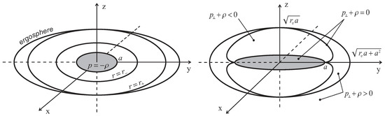
Figure 1.
Left: Horizons, ergosphere, and the interior de Sitter vacuum disk for a de Sitter-Kerr black hole with the first type of interior. Right: Vacuum -surface for the de Sitter-Kerr black hole with the second type of interior. In Figure 1 energy density is denoted by ( in the units ).
The weak energy condition can be in principle violated beyond the vacuum surface on which . It is possible in the case when in Equation (12), which in turn is possible only if a related spherical solution satisfies the dominant energy condition. Then there can exist the -surface, defined by , which contains the de Sitter disk as a bridge. The weak energy condition is violated in the internal cavities between the -surface and the disk, which are filled thus with an anisotropic phantom fluid, with . This is the second type of interior shown in Figure 1 Right [34], where is the regularity parameter for the case admitting this type of interior (more details in Section 4).
3. Shadows of Regular de Sitter-Kerr Black Holes
3.1. Integrals of Motion Defining the Boundary of Shadow
The basic parameters related to the integrals of motion on the photon geodesics are defined by [1]
where the integrals of motion E and are related to the Killing vectors and in the axially symmetric geometry (6).
The integral of motion Q is related to the quadratic integral of motion given by [1]
and related to the conformal Killing tensor existing in a spacetime of D-type of Petrov classification ([1] and references therein).
The photon geodesics satisfy the equations
where dot denotes the derivative with respect to the affine parameter along a geodesic.
The innermost unstable photon orbits which define the boundary of the shadow are defined by two equations
From these equations we find the relation between the parameters and on the orbits
and obtain the equation for
where
The determinant of Equation (18) reduces to the form
The resulting general formulae for the integrals of motion and on the orbits read
For they coincide with those for the Kerr metric presented in [1].
3.2. Information About a Black Hole from Its Shadow
The celestial coordinates related with the integrals of motion for the innermost orbits [1], correspond to the impact parameters for the boundary of the gravitational capture cross-section as seen by an observer at infinity, since photons infalling with these impact parameters get to the innermost unstable photon orbits [1,2]
Here is the angular coordinate of an observer; x is the apparent distance of the black hole image from the symmetry axis perpendicular to it; y the apparent distance of the black hole image from its projection on the equatorial plane, perpendicular to it. Introduction of the impact parameters is shown in Figure 2 Left, where .
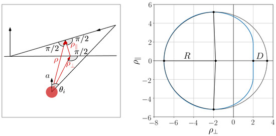
Figure 2.
Left: Impact parameters and corresponding to the celestial coordinates . Right: Asymmetry parameter D.
To determine the asymmetry of the shadow we construct the fitting circle with the radius R and the center at , using the coordinates of the upper point of the shadow contour and of its left and right endpoints in the equatorial plane, and . The asymmetry parameter D is introduced as the distance between the right endpoints of the circle and of the shadow contour [7] as shown in Figure 2 Right, where , and . Eliminating , we obtain the radius of the fitting circle
and the distortion parameter
Equations (22) and (23) defining the contour of the shadow, can be written in the simpler form with using the integral given by (14) in terms of and , which reads
In the celestial coordinates
and Equation (28) yield
Introducing the variables
we transform the system (28) to
From the first equation we find
Differentiating equations of the system (32) with respect to u we obtain
which gives the equation for the derivative (for y and x related by the curve for the boundary of the shadow)
Taking into account Equations (31) and (33) we obtain the derivative on the shadow boundary dependently on the functions defining the unstable orbits forming the boundary
As a result, the upper point of the shadow contour is determined by the system of Equations (37) and (38).
For an observer coordinate () this system reduces to the simple form
Here and in what follows, distances are normalized to the mass parameter M and , where is the mass function normalized to M. For the Kerr black hole and we obtain in agreement with the known results (see, e.g., [1]).
The left and right points of the shadow contour correspond to , and Equation (30) gives the equation for the innermost orbit in the equatorial plane
Multiplying by , we obtain
Introducing the new variable
we obtain the cubic equation
For the equation in the canonical form with the coefficients
solutions are determined by the quantities
Types of solutions depend on the signs of q and S. For the constant mass the solutions should coincide with those for the Kerr black hole, for which and . We can expect that the shape of a shadow for a regular black hole would not differ essentially from that for the Kerr black hole and assume that and . Then Equation (43) has 3 real roots defined by
Taking into account (42) we obtain the transcendental equation for r
which gives the orbit radii forming the boundary of the shadow in the equatorial plane for an arbitrary regular axially symmetric metric
In the case of the Kerr metric , , and Equation (48) yields
in agreement with [1]. It follows that applies to the retrograde orbit while to the direct orbit. We can conclude that in general case the solutions specified by and in Equation (48) represent the radii of the retrograde and direct orbits, respectively, for an arbitrary axially symmetric metric.
The shadow contour is calculated numerically for different values of the observer coordinate . The spin of a black hole is determined from the relation between its spin and the distortion parameter for the boundary of its shadow.
In the equatorial plane the relation between the celestial coordinate x and the orbit radius r can be found by considering the innermost equatorial photon orbits which are specified by
are described by the function in Equation (15) which reduces to
and obey the system of equations in Equation (16), in the form
This gives
Ultimately we obtain for the celestial coordinate x
For each value of k in Equation (48) we can now obtain and and determine the boundary of the shadow in the equatorial plane.
Equation (54) with account of for the considered class of metrics, gives the basic constraint
which suggests that (i) the shadow of a regular black should have to be smaller than that for the Kerr black hole, and (ii) the difference depends essentially on the density profile of a regular black hole.
Comparison of a black hole shadow with using de Sitter-Kerr metric for fitting its boundary, with the Kerr shadow can provide information about interior structure of a black hole.
4. Shadows for Two Particular Regular Black Holes
Black hole regularized by vacuum polarization effects— In the first particular solution with the de Sitter interior [28] the basic idea is that since all fields are involved in a gravitational collapse this does not allow one to calculate it carefully, but at the same time this implies that all of them contribute to the gravitational field via the Einstein equations, so that we can evaluate the vacuum polarization in a resulting spherical gravitational field.
In the simple semiclassical model this gives the density profile and the mass function [28,30,36]
Normalizing to , distances and the mass function to M, we get the dimensionless energy density and the dimensionless mass function
-function in the dimensionless form defines the event horizon by the root of the equation dependently on the couple of parameters . This range of parameters is used for numerical investigation of the shadow.
The parameter a is taken within the range from 0 to 1. For each a we find the critical value of beyond which the equation does not have positive roots. The results are shown in Table 1 and in Figure 3 Left, where we also show the case of the Kerr black hole for comparison (Figure 3 Right).

Table 1.
The event horizons for different values of the parameters a and .
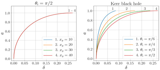
Figure 3.
Left: Relation between spin and distortion parameter for an observer with . Right: Relation between spin and distortion parameter for the Kerr black hole.
As we can see, in the case of the quickly decreasing polarization profile Equation (57) the curves in Figure 3 Left do not depend on the parameter and actually coincide with the curve for the Kerr black hole (the curve 4 in Figure 3 Right).
Black hole with the regularized Newtonian profile— The phenomenologically regularized Newtonian profile is defined as [37]
For this density profile provides the cut-off on self-interaction by the density at . The cut-off length scale gives which corresponds to related to the de Sitter core, in accordance with the Zel’dovich idea [38] to associate cosmological constant with the energy density of self-interaction. The interior density is related with the total mass M by the formula where the length scale is characteristic for de Sitter-Schwarzschild geometry matching directly [39] or continuously [28,29] the Schwarzschild exterior to the de Sitter interior.
For estimates we adopt the GUT scale GeV which gives cm. Normalizing on M gives the dimensionless mass function and the cut-off parameter
Table 2.
The event horizons for different values of the parameters a, and .
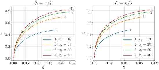
Figure 4.
Left: Relation between the spin a and the distortion parameter for . Right: Relation between the spin a and the distortion parameter for .
In the next Section we present the comparative analysis for these two particular regular black holes which differ by the pace of the density decreasing.
5. Comparison of Shadows for Black Holes with Quickly and Slowly Decreasing Densities
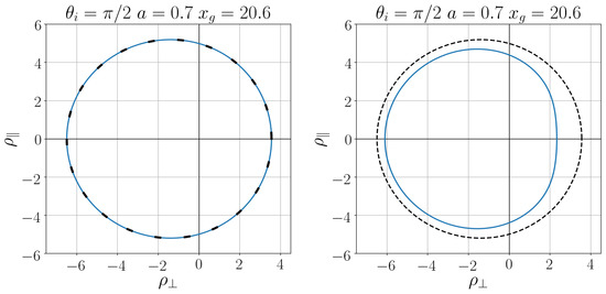
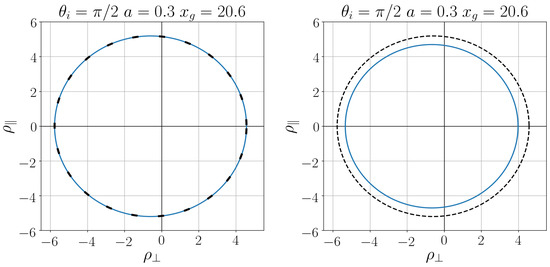
Shadows of two regular black holes, [28,34], in comparison with the Kerr black hole are shown in Figure 5 and Figure 6 for two values of the black hole spin, and . They differ by the pace of decreasing of the density profile. In the first case the density (56) is quickly decreasing, and the shadow of the regular black hole practically coincides with that for the Kerr black hole. In the second case the density (58) decreases slowly, and we see the marked difference between the regular black hole shadow and the Kerr black hole shadow.
Relation between the regularization parameter and the distortion parameter is shown in Figure 7 and Figure 8 for two values of the black hole spin, and . The vertical dashed lines refer to the Kerr black hole.
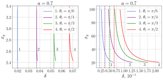
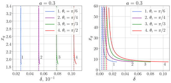
For the black hole with the quickly decreasing polarization profile (56) the distortion parameter starts to coincide with that for the Kerr black hole already for small values of (small masses), so that for astrophysical black holes it evidently coincides with that for the Kerr black hole. For the black hole with the slowly decreasing regularized Newtonian profile (58) difference of the distortion parameter from that for the Kerr black hole is more noticeable.
6. Conclusions
We present the basic general formulae which describe shadows of regular rotating black holes obtained from regular spherical solutions with using the Newman–Janis algorithm. Regular black hole solutions are specified by , belong to the Kerr–Schild class, and have the de Sitter vacuum disk in their deep interiors. In the case where a related spherical solution satisfies the dominant energy condition, the de Sitter disk is embedded inside a closed de Sitter vacuum -surface. The weak energy condition is violated in the internal cavities between -surface and the de Sitter disk, which are filled with an anisotropic phantom fluid.
The information on the interior content of a regular rotating black hole of this class can be in principle extracted from observation of its shadow.
We show that for regular de Sitter-Kerr black holes the boundary of the shadow and the distortion parameter characterizing its asymmetry depend essentially on the interior density. Their shadows are typically smaller than that for the Kerr black hole with the same mass and spin, and the difference depends on the form of the density profile.
Numerical analysis for two particular black holes of this class reveals that the difference between the Kerr black hole shadow and a regular black hole shadow depends essentially on the pace of density decreasing. The shadow of a regular black hole with quickly decreasing density can coincide with the shadow of the Kerr black hole. For a regular black hole with slowly decreasing density the difference between its shadow and the Kerr shadow can be substantial.
We can hope that the comprehensive analysis of the observed black hole shadow with using different metrics for fitting its boundary, would give a certain information on the nature of the black hole interior.
Author Contributions
Authors contributed equally to this work.
Funding
This research received no external funding.
Conflicts of Interest
The authors declare no conflict of interest.
References
- Chandrasekhar, S. The Mathematical Theory of Black Holes; Clarendon Press: Oxford, UK, 1983. [Google Scholar]
- Dymnikova, I.G. Motion of particles and photons in the gravitational field of a rotating body (In memory of Vladimir Afanas’evich Ruban). Sov. Phys. Uspekhi 1986, 29, 215–237. [Google Scholar] [CrossRef]
- Falcke, H.; Melia, F.; Agol, E. Viewing the shadow of the black hole at the Galactic Center. Astrophys. J. Lett. 2000, 528, L13–L16. [Google Scholar] [CrossRef]
- Takahashi, R. Shapes and positions of black hole shadows in accretion disks and spin parameters of black holes. Astrophys. J. 2004, 611, 996–1004. [Google Scholar] [CrossRef]
- Doeleman, S.S.; Weintroub, J.; Rogers, A.E.E.; Plambeck, R.; Freund, R.; Tilanus, R.P.J.; Friberg, P.; Ziurys, L.M.; Moran, J.M.; Corey, B.; et al. Event-horizon-scale structure in the supermassive black hole candidate at the Galactic Center. Nature 2008, 455, 78–80. [Google Scholar] [CrossRef] [PubMed]
- Alberdi, A.; Gómez Fernández, J.L.; The Event Horizon Telescope Collaboration. First M87 Event Horizon Telescope Results. I. The Shadow of the Supermassive Black Hole. Astrophys. J. Lett. 2019, 875, L1. [Google Scholar]
- Hioki, K.; Maeda, K. Measurement of the Kerr spin parameter by observation of a compact object’s shadow. Phys. Rev. D 2009, 80, 024042. [Google Scholar] [CrossRef]
- Li, Z.; Bambi, C. Measuring the Kerr spin parameter of regular black holes from their shadow. J. Cosmol. Astropart. Phys. 2014, 2014, 41–61. [Google Scholar] [CrossRef]
- Grenzebach, A. Aberration effects for shadows of black holes. Fundam. Theor. Phys. 2015, 179, 823–832. [Google Scholar]
- Mars, K.; Paganini, C.F.; Oancea, M.A. The fingerprints of black holes - shadows and their degeneracies. Class. Quant. Grav. 2018, 35, 025005. [Google Scholar] [CrossRef]
- Grenzebach, A.; Perlick, V.; Lámmerzahl, C. Photon regions and shadows of Kerr-Newman-NUT black holes with a cosmological constant. Phys. Rev. 2014, D89, 124004. [Google Scholar] [CrossRef]
- Repin, S.V.; Kompaneets, D.A.; Novikov, I.D.; Mityagina, V.A. Shadow of rotating black holes on a standard background screen. arXiv 2018, arXiv:1802.04667 [gr-qc]. [Google Scholar]
- Bambi, C.; Freese, K. Apparent shape of super-spinning black holes. Phys. Rev. D 2009, 79, 043002. [Google Scholar] [CrossRef]
- Bambi, C.; Yoshida, N. Shape and position of the shadow in the ? = 2 Tomimatsu-Sato spacetime. Class. Quant. Grav. 2010, 27, 205006. [Google Scholar] [CrossRef]
- Johannsen, T.; Psaltis, D. Testing the No-Hair theorem with observations in the electromagnetic specrum. II. Black hole images. Astrophys. J. 2010, 718, 446–454. [Google Scholar] [CrossRef]
- Ayon-Beato, A.; Garcia, A. The Bardeen model as a nonlinear magnetic monopole. Phys. Lett. B 2000, 493, 149–152. [Google Scholar] [CrossRef]
- Hayward, S.A. Formation and evaporation of nonsingular black holes. Phys. Rev. Lett. 2006, 96, 031103–031105. [Google Scholar] [CrossRef] [PubMed]
- Mizuno, Y.; Younsi, Z.; Fromm, C.M.; Porth, O.; De Laurentis, M.; Olivares, H.; Falcke, H.; Kramer, M.; Rezzolla, L. The current ability to test theories of gravity with black hole shadows. Nat. Astron. Lett. 2018, 2, 585–590. [Google Scholar] [CrossRef]
- Younsi, Z.; Wu, K.; Fuerst, S.V. General relativistic radiative transfer: formulation and emission from structured tori around black holes. Astron. Astrophys. 2012, 545, A13. [Google Scholar] [CrossRef]
- Chan, C.-K.; Psaltis, D.; Oezel, F.; Narayan, R.; Sadowski, A. The power of imaging: constraining the plasma properties of GRMHD simulations using EHT observations of Sgr A*. Astrophys. J. 2015, 799, 1. [Google Scholar] [CrossRef]
- Rezzolla, L.; Zhidenko, A. New parametrization for spherically symmetric black holes in metric theories of gravity. Phys. Rev. D 2014, 90, 084009. [Google Scholar] [CrossRef]
- Garca, A.; Galtsov, D.; Kechkin, O. Class of stationary axisymmetric solutions of the Einstein-Maxwell-dilaton-axion field equations. Phys. Rev. Lett. 1995, 74, 1276–1279. [Google Scholar] [CrossRef] [PubMed]
- Cunha, P.V.P.; Herdeiro, C.A.R. Shadows and strong gravitational lensing: A brief review. Gen. Rel. Grav. 2018, 50, 42. [Google Scholar] [CrossRef]
- Newman, E.T.; Janis, A.J. Note on the Kerr Spinning-Particle Metric. J. Math. Phys. 1965, 6, 915–917. [Google Scholar] [CrossRef]
- Gürses, M.; Gürsey, F. Lorentz covariant treatment of the Kerr-Schild geometry. J. Math. Phys. 1975, 16, 2385–2391. [Google Scholar] [CrossRef]
- Kerr, R.P.; Schild, A. Some algebraically degenerate solutions of Einstein’s gravitational field equations. Proc. Symp. Appl. Math. 1965, 17, 199. [Google Scholar]
- Shaikh, R. Black hole shadow in a general rotating spacetime obtained through Newman-Janis algorithm. arXiv 2019, arXiv:1904.08322 [gr-qc]. [Google Scholar]
- Dymnikova, I. Vacuum nonsingular black hole. Gen. Rel. Grav. 1992, 24, 235–242. [Google Scholar] [CrossRef]
- Dymnikova, I. The algebraic structure of a cosmological term in spherically symmetric solutions. Phys. Lett. B 2000, 472, 33–38. [Google Scholar] [CrossRef]
- Dymnikova, I. The cosmological term as a source of mass. Class. Quant. Grav. 2002, 19, 725–740. [Google Scholar] [CrossRef]
- Dymnikova, I. Spherically symmetric space-time with regular de Sitter center. Int. J. Mod. Phys. D 2003, 12, 1015–1034. [Google Scholar] [CrossRef]
- Burinskii, A.; Elizalde, E.; Hildebrandt, S.R.; Magli, G. Regular sources of the Kerr-Schild class for rotating and nonrotating black hole solutions. Phys. Rev. D 2002, 65, 064039. [Google Scholar] [CrossRef]
- Dymnikova, I. Spinning superconducting electrovacuum soliton. Phys. Lett. B 2006, 639, 368–372. [Google Scholar] [CrossRef]
- Dymnikova, I.; Galaktionov, E. Regular rotating de Sitter-Kerr black holes and solitons. Class. Quant. Grav. 2016, 33, 145010. [Google Scholar] [CrossRef]
- Dymnikova, I.; Galaktionov, E. Basic Generic Properties of Regular Rotating Black Holes and Solitons. Adv. Math. Phys. 2017, 2017, 1035381. [Google Scholar] [CrossRef]
- Dymnikova, I. De Sitter-Schwarzschild black hole: Its particlelike core and thermodynamical properties. Int. J. Mod. Phys. D 1996, 5, 529–540. [Google Scholar] [CrossRef]
- Dymnikova, I. Regular electrically charged vacuum structures with de Sitter center in nonlinear electrodynamics coupled to general relativity. Class. Quant. Grav. 2004, 21, 4417–4428. [Google Scholar] [CrossRef]
- Zel’dovich, Y.B. Cosmological constant and elementary particles. JETP Lett. 1967, 6, 883–884. [Google Scholar] [CrossRef]
- Poisson, E.; Israel, W. Structure of the black hole nucleus. Class. Quant. Grav. 1988, 5, L201–L205. [Google Scholar] [CrossRef]
| 1 | Generalization of the Newman–Janis algorithm to the more general case has been considered in [27]. |


© 2019 by the authors. Licensee MDPI, Basel, Switzerland. This article is an open access article distributed under the terms and conditions of the Creative Commons Attribution (CC BY) license (http://creativecommons.org/licenses/by/4.0/).