Quantum Optimal Control of Rovibrational Excitations of a Diatomic Alkali Halide: One-Photon vs. Two-Photon Processes

Abstract
1. Introduction
2. Theoretical Details
2.1. OCT
2.2. Wave-Packet Propagation
3. Results and Discussion
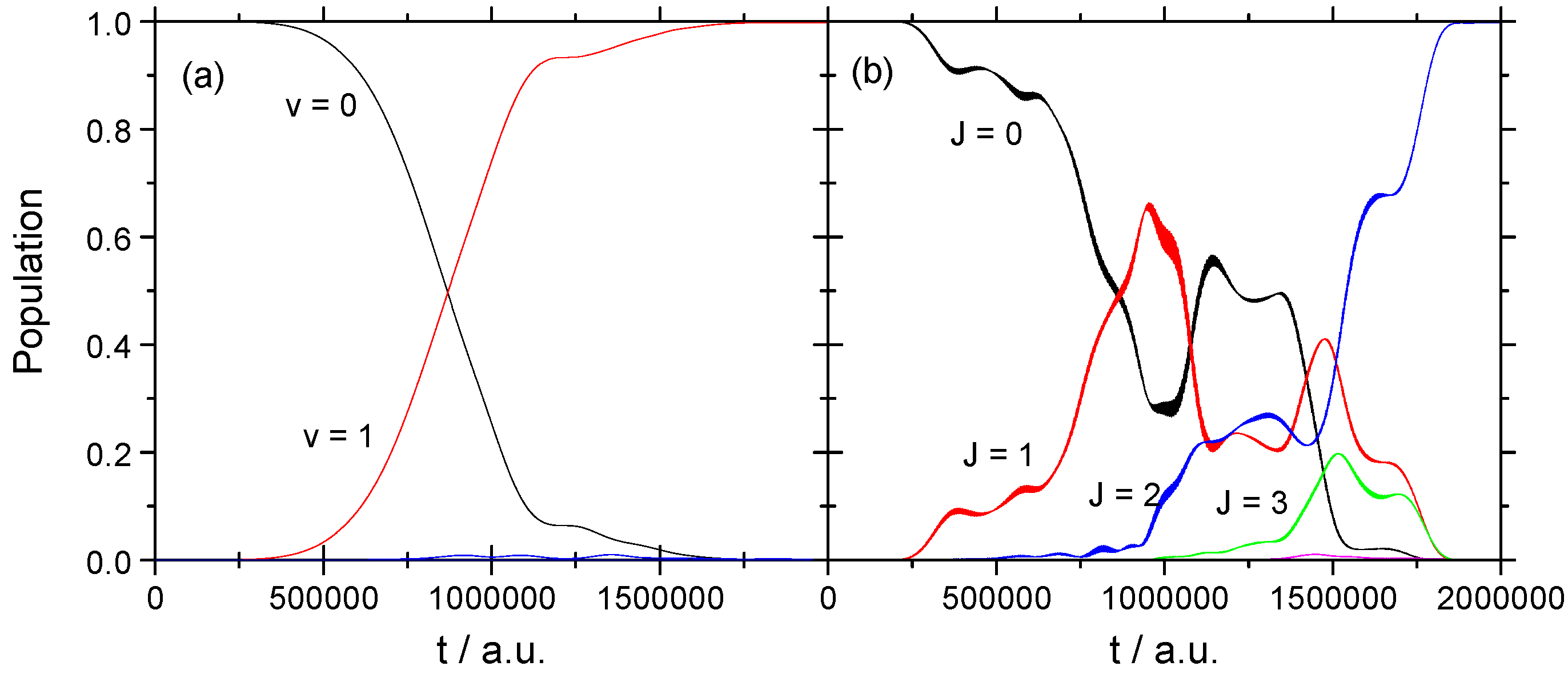
3.1. Rotational Excitation: (v = 0, J = 0) → (v = 0, J = 2)
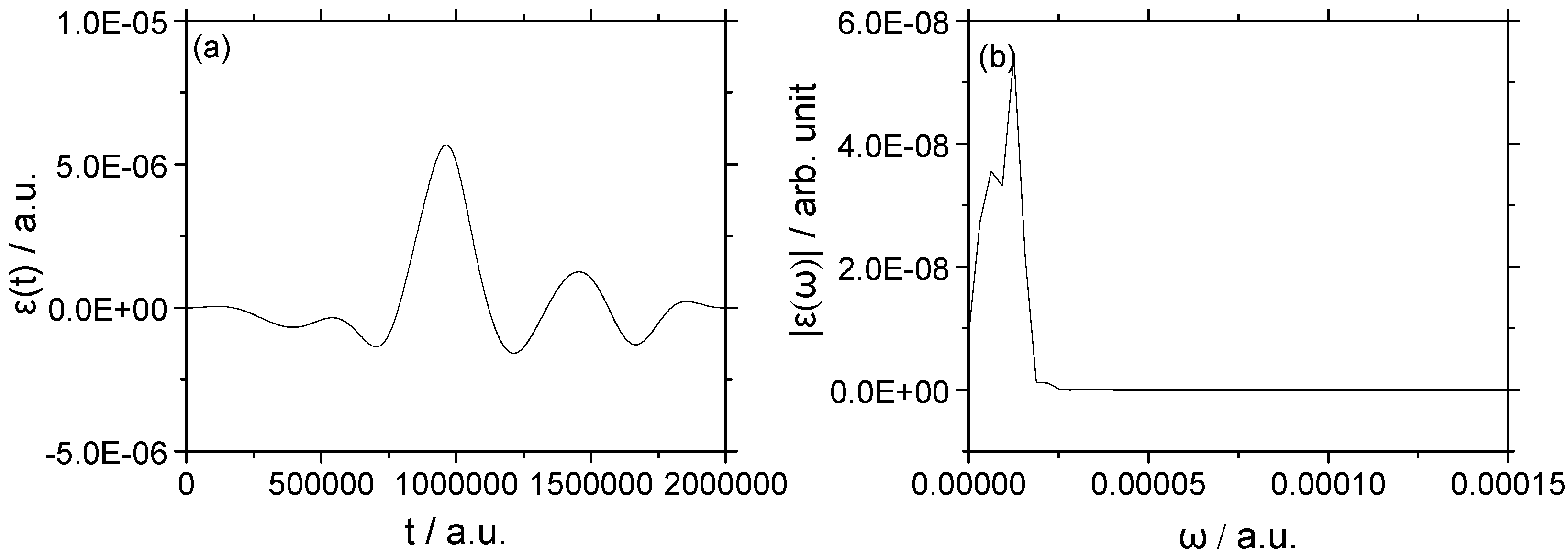
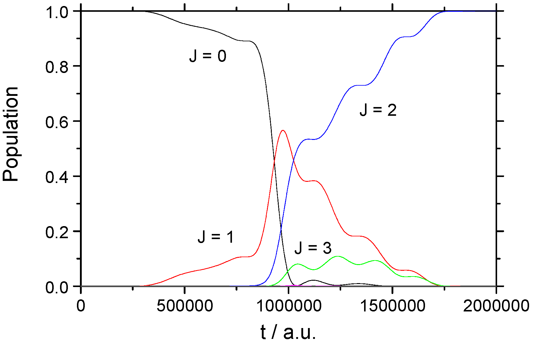
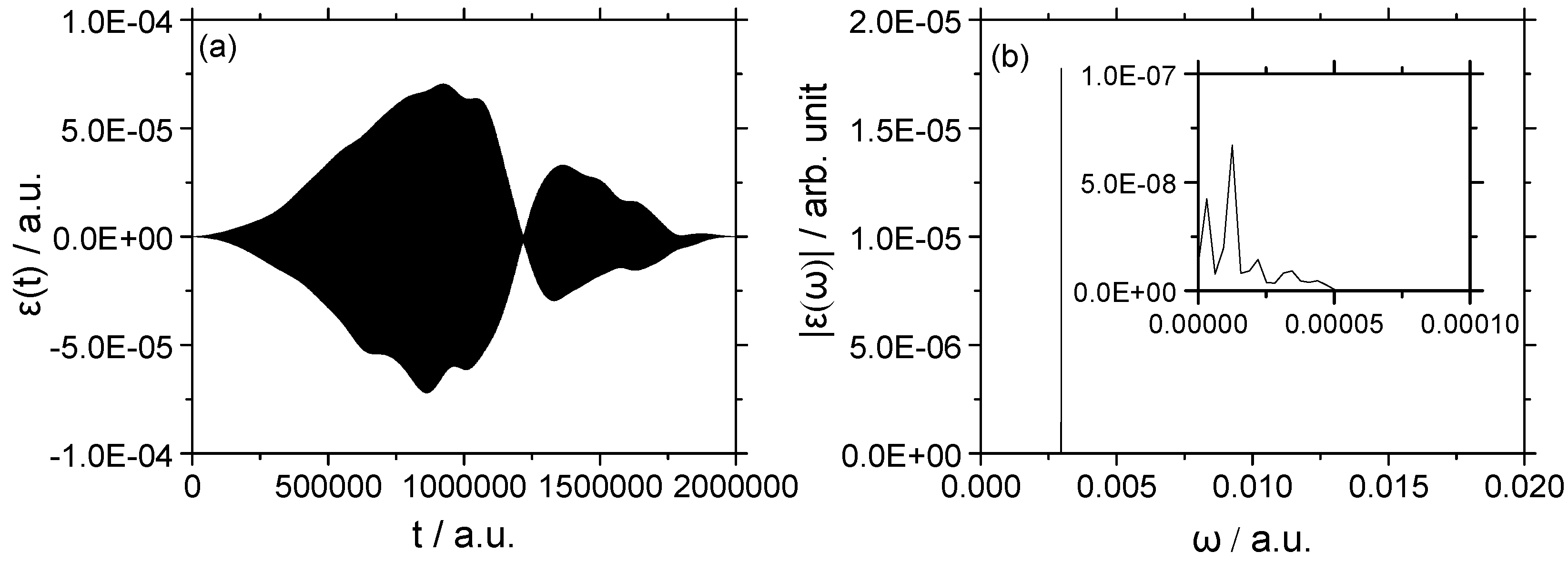
3.1.1. Weak Field
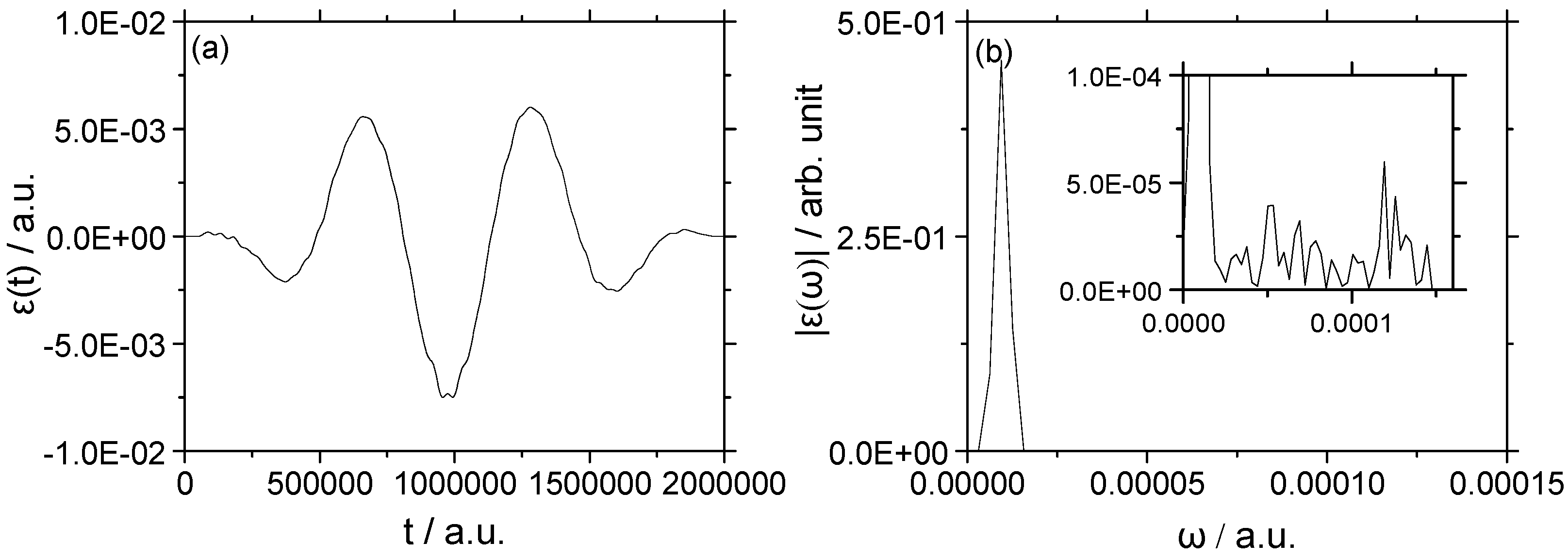
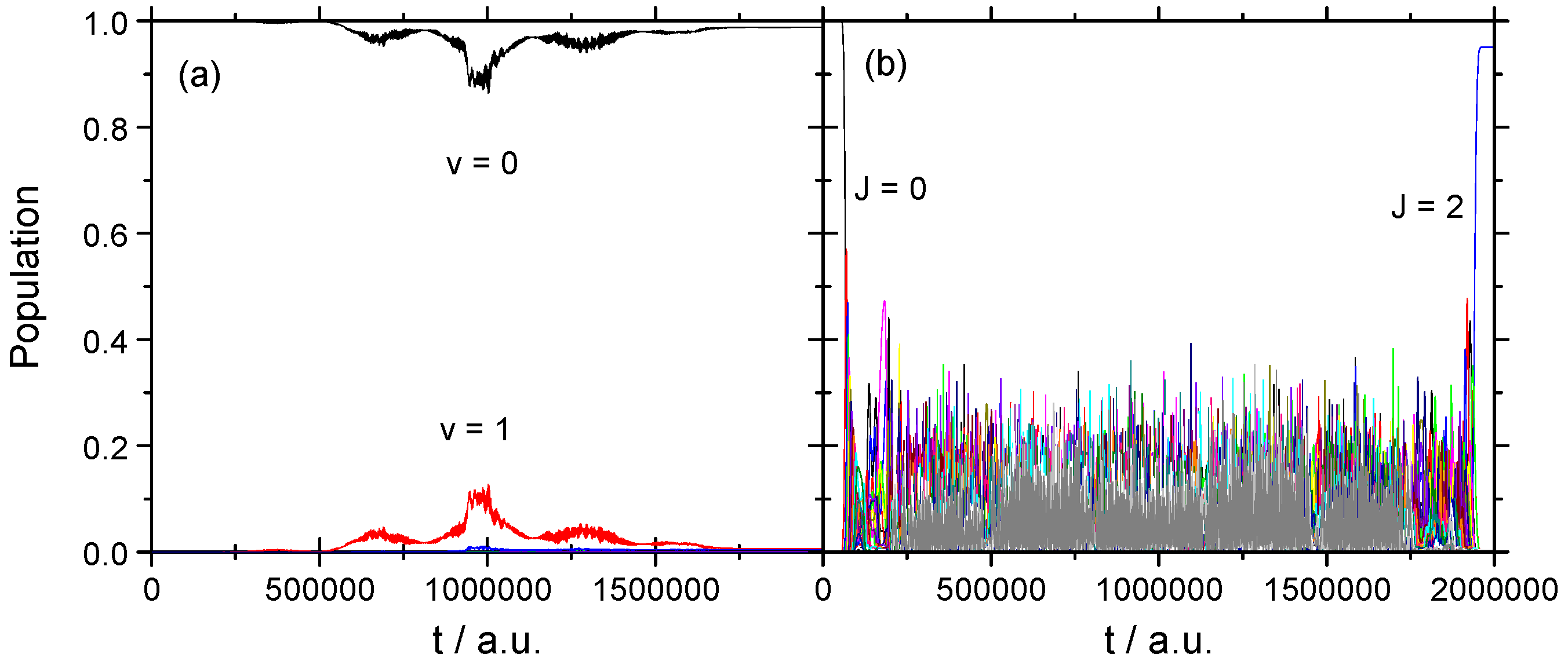
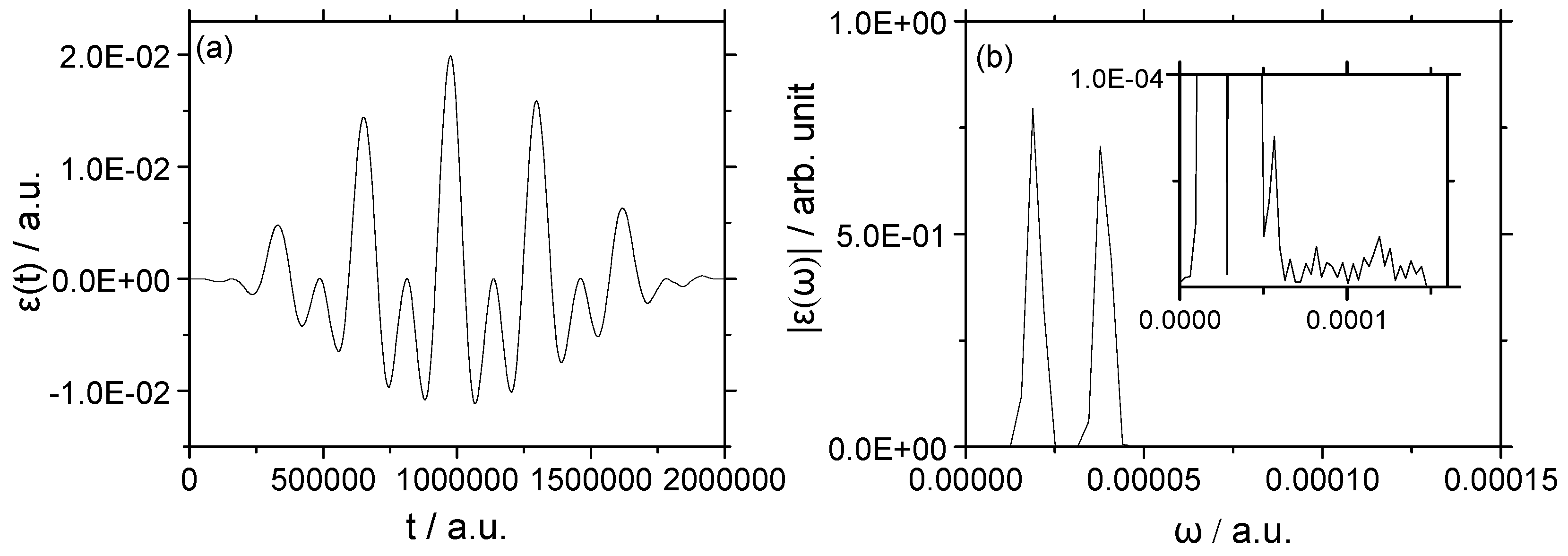
3.1.2. Strong Field
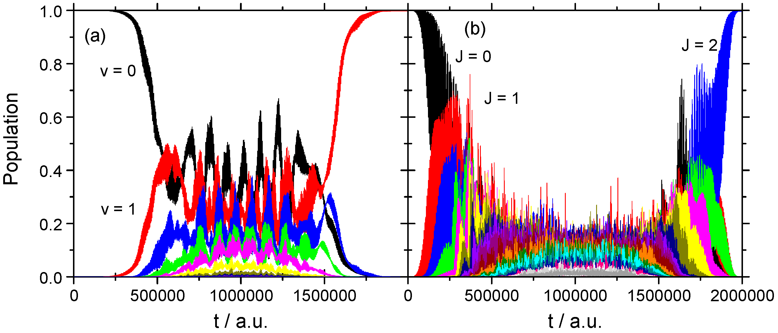
3.2. Vibrational–Rotational Excitation: (v = 0, J = 0) → (v = 1, J = 2)
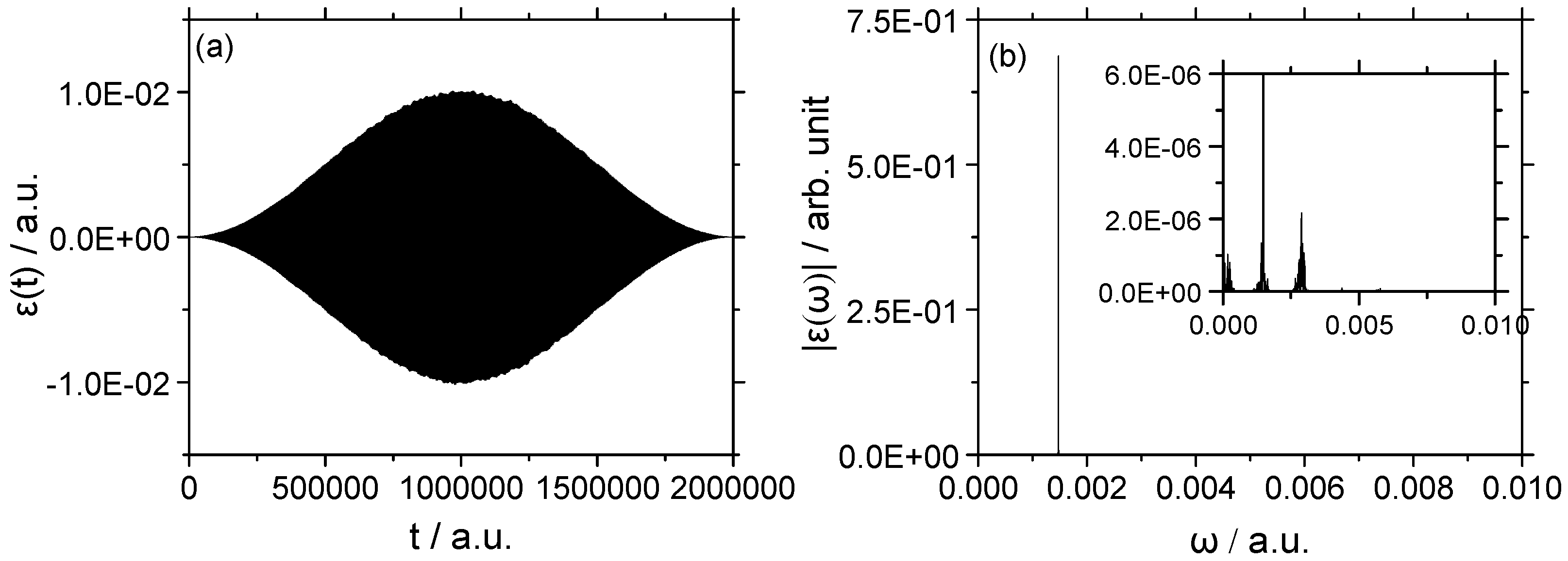
3.2.1. Weak Field
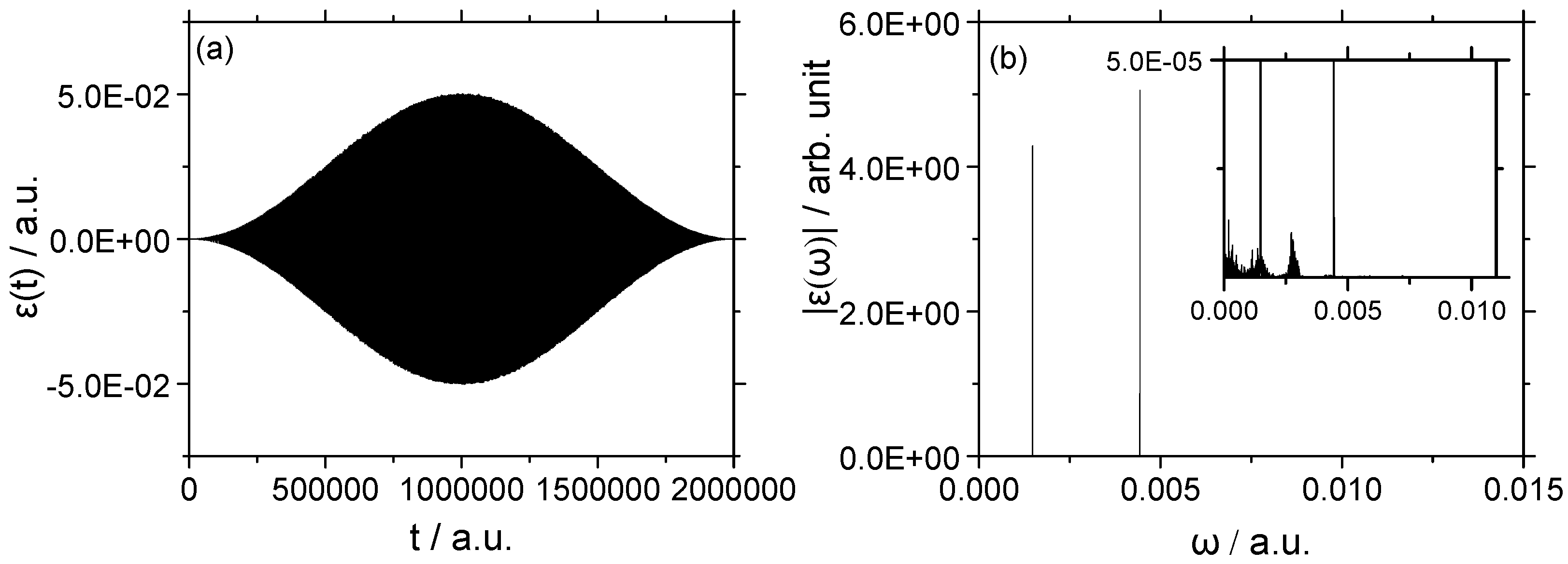
3.2.2. Strong Field
4. Conclusions
Supplementary Materials
Author Contributions
Funding
Acknowledgments
Conflicts of Interest
References
- Rice, S.A.; Zhao, M. Optical Control of Molecular Dynamics; Wiley: New York, NY, USA, 2000. [Google Scholar]
- Letokhov, V.S. Laser Control of Atoms and Molecules; Oxford University Press: New York, NY, USA, 2007. [Google Scholar]
- D’alessandro, D. Introduction to Quantum Control and Dynamics; Chapman & Hall: London, UK, 2007. [Google Scholar]
- Shapiro, M.; Brumer, P. Quantum Control of Molecular Processes; Wiley-VCH: Weinheim, Germany, 2012. [Google Scholar]
- Kosloff, R.; Rice, S.A.; Gaspard, P.; Tersigni, S.; Tannor, D.J. Wavepacket dancing: Achieving chemical selectivity by shaping light pulses. Chem. Phys. 1989, 139, 201–220. [Google Scholar] [CrossRef]
- Brumer, P.; Shapiro, M. Coherence chemistry: Controlling chemical reactions with lasers. Acc. Chem. Res. 1989, 22, 407–413. [Google Scholar] [CrossRef]
- Stapelfeldt, H.; Seideman, T. Aligning molecules with strong laser pulses. Rev. Mod. Phys. 2003, 75, 543. [Google Scholar] [CrossRef]
- Nielsen, M.A.; Chuang, I.L. Quantum Computation and Quantum Information; Cambridge University Press: Cambridge, UK, 2000. [Google Scholar]
- Bartana, A.; Kosloff, R.; Tannor, D.J. Laser cooling of molecular internal degrees of freedom by a series of shaped pulses. J. Chem. Phys. 1993, 99, 196–210. [Google Scholar] [CrossRef]
- McCarron, D.J.; Steinecker, M.H.; Zhu, Y.; DeMille, D. Magnetic trapping of an ultracold gas of polar molecules. Phys. Rev. Lett. 2018, 121, 013202. [Google Scholar] [CrossRef] [PubMed]
- Bergmann, K.; Theuer, H.; Shore, B.W. Coherent population transfer among quantum states of atoms and molecules. Rev. Mod. Phys. 1998, 70, 1003. [Google Scholar] [CrossRef]
- Vitanov, N.V.; Rangelov, A.A.; Shore, B.W.; Bergmann, K. Stimulated Raman adiabatic passage in physics, chemistry, and beyond. Rev. Mod. Phys. 2017, 89, 015006. [Google Scholar] [CrossRef]
- Falci, G.; Di Stefano, P.G.; Ridolfo, A.; D’Arrigo, A.; Paraoanu, G.S.; Paladino, E. Advances in quantum control of three-level superconducting circuit architectures. Prog. Phys. 2017, 65, 1600077. [Google Scholar] [CrossRef]
- Torrontegui, E.; Ibánez, S.; Martínez-Garaot, S.; Modugno, M.; del Campo, A.; Guéry-Odelin, D.; Ruschhaupt, A.; Chen, X.; Muga, J.G. Shortcuts to adiabaticity. Adv. At. Mol. Opt. Phys. 2013, 62, 117–169. [Google Scholar]
- Vepsäläinen, A.; Danilin, S.; Paraoanu, G.S. Optimal superadiabatic population transfer and gates by dynamical phase corrections. Quantum Sci. Technol. 2018, 3, 024006. [Google Scholar] [CrossRef]
- Vepsäläinen, A.; Danilin, S.; Paraoanu, G.S. Superadiabatic population transfer in a three-level superconducting circuit. Sci. Adv. 2019, 5, eaau5999. [Google Scholar] [CrossRef]
- Shi, S.; Rabitz, H. Quantum mechanical optimal control of physical observables in microsystems. J. Chem. Phys. 1990, 92, 364–376. [Google Scholar] [CrossRef]
- Zhu, W.; Botina, J.; Rabitz, H. Rapidly convergent iteration methods for quantum optimal control of population. J. Chem. Phys. 1998, 108, 1953–1963. [Google Scholar] [CrossRef]
- Sundermann, K.; de Vivie-Riedle, R. Extensions to quantum optimal control algorithms and applications to special problems in state selective molecular dynamics. J. Chem. Phys. 1999, 110, 1896–1904. [Google Scholar] [CrossRef]
- Levis, R.; Rabitz, H. Closing the loop on bond selective chemistry using tailored strong field laser pulses. J. Phys. Chem. A 2002, 106, 6427–6444. [Google Scholar] [CrossRef]
- Herek, J.L.; Wohllenben, W.; Cogdell, R.J.; Zeldler, D.; Motzkus, M. Quantum control of energy flow in light harvesting. Nature 2002, 417, 533–535. [Google Scholar] [CrossRef]
- Kurosaki, Y.; Yokoyama, K.; Yokoyama, A. Multilevel effect on ultrafast isotope-selective vibrational excitations: Quantum optimal control study. J. Mol. Struct. Theochem. 2009, 913, 38–42. [Google Scholar] [CrossRef]
- Kurosaki, Y.; Yokoyama, K.; Yokoyama, A. Quantum control study of multilevel effect on ultrafast isotope-selective vibrational excitations. J. Chem. Phys. 2009, 131, 144305. [Google Scholar] [CrossRef]
- Kurosaki, Y.; Yokoyama, K.; Yokoyama, A. Quantum control study of ultrafast isotope-selective vibrational excitations of the cesium iodide (CsI) molecule. Comput. Theoret. Chem. 2011, 963, 245–255. [Google Scholar] [CrossRef]
- Kurosaki, Y.; Ichihara, A.; Yokoyama, K. Quantum optimal control for the full ensemble of randomly oriented molecules having different field-free Hamiltonians. J. Chem. Phys. 2011, 135, 054103. [Google Scholar] [CrossRef]
- Yokoyama, K.; Matsuoka, L.; Kasajima, T.; Tsubouchi, M.; Yokoyama, A. Quantum control of molecular vibration and rotation toward the isotope separation. In Advances in Intense Laser Science and Photonics; Lee, J., Ed.; Publishing House for Science and Technology: Hanoi, Vietnam, 2010; p. 113. [Google Scholar]
- Matsuoka, L.; Ichihara, A.; Hashimoto, M.; Yokoyama, K. Theoretical study for laser isotope separation of heavy-element molecules in a thermal distribution. In Proceedings of the International Conference on toward and over the Fukushima Daiichi Accident (GLOBAL 2011), Tokyo, Japan, 11–16 December 2011. [Google Scholar]
- Ichihara, A.; Matsuoka, L.; Kurosaki, Y.; Yokoyama, K. Theoretical study on isotope-selective dissociation of the lithium chloride molecule using a designed terahertz-wave field. In Proceedings of the 12th Asia Pacific Physics Conference (APPC12), Chiba, Japan, 14–19 July 2013; p. 013093. [Google Scholar]
- Ichihara, A.; Matsuoka, L.; Kurosaki, Y.; Yokoyama, K. An analytic formula to describe transient rotational dynamics of diatomic molecules in an optical frequency comb. Chin. J. Phys. 2013, 51, 1230–1340. [Google Scholar]
- Ichihara, A.; Matsuoka, L.; Kurosaki, Y.; Yokoyama, K. Quantum control of isotope-selective rovibrational excitation of diatomic molecules in the thermal distribution. Opt. Rev. 2015, 22, 153–156. [Google Scholar] [CrossRef]
- Kurosaki, Y.; Yokoyama, K. Quantum optimal control of the isotope-selective rovibrational excitation of diatomic molecules. Chem. Phys. 2017, 493, 183–193. [Google Scholar] [CrossRef]
- Ohtsuki, Y.; Nakagami, K. Monotonically convergent algorithms for solving quantum optimal control problems of a dynamical system nonlinearly interacting with a control. Phys. Rev. A 2008, 77, 033414. [Google Scholar] [CrossRef]
- Abe, H.; Ohtsuki, Y. Frequency-network mechanism for alignment of diatomic molecules by multipulse excitation. Phys. Rev. A 2011, 83, 053410. [Google Scholar] [CrossRef]
- Kurosaki, Y.; Yokoyama, K. Ab initio MRSDCI study on the low-lying electronic states of the lithium chloride molecule (LiCl). J. Chem. Phys. 2012, 137, 064305. [Google Scholar] [CrossRef]
- Frisch, M.J.; Trucks, G.W.; Schlegel, H.B.; Scuseria, G.E.; Robb, M.A.; Cheeseman, J.R.; Scalmani, G.; Barone, V.; Mennucci, B.; Petersson, G.A.; Revision, D.; et al. Gaussian 09; Revision D.01; Gaussian, Inc.: Wallingford, CT, USA, 2013. [Google Scholar]
- Marston, C.C.; Balint-Kurti, G.G. The Fourier grid Hamiltonian method for bound state eigenvalues and eigenfunctions. J. Chem. Phys. 1989, 91, 3571–3576. [Google Scholar] [CrossRef]
- Press, W.H.; Flannery, B.P.; Teukolsky, S.A.; Vetterling, T. Numerical Recipes; Cambridge University Press: Cambridge, MA, USA, 1986. [Google Scholar]
- Feit, M.D.; Fleck, J.A., Jr.; Steiger, A. Solution of the Schrödinger equation by a spectral method. J. Comput. Phys. 1982, 47, 412–433. [Google Scholar] [CrossRef]
- Feit, M.D.; Fleck, J.A., Jr. Solution of the Schrödinger equation by a spectral method II: Vibrational energy levels of triatomic molecules. J. Chem. Phys. 1983, 78, 301–308. [Google Scholar] [CrossRef]
- Feit, M.D.; Fleck, J.A., Jr. Wave packet dynamics and chaos in the Hénon–Heiles system. J. Chem. Phys. 1984, 80, 2578–2584. [Google Scholar] [CrossRef]
- Light, J.C.; Hamilton, I.P.; Lill, V.J. Generalized discrete variable approximation in quantum mechanics. J. Chem. Phys. 1985, 82, 1400–1409. [Google Scholar] [CrossRef]
- Dai, J.; Light, J.C. A grid representation for spherical angles: Decoupling of the angular momentum operator. J. Chem. Phys. 1997, 107, 8432–8436. [Google Scholar] [CrossRef]
- Mahapatra, S.; Sathyamurthy, N. Negative imaginary potentials in time-dependent quantum molecular scattering. J. Chem. Soc. Faraday Trans. 1997, 93, 773–779. [Google Scholar] [CrossRef]


| Parameter | Value |
|---|---|
| Range of the Li-Cl bond length (bohr) | 2.2677–5.6692 |
| Number of radial grid points | 32 |
| Number of angular grid points | 20 |
| Total time (a.u.) | 2,000,000 |
| Number of time steps | 131,072 |
| Init. Guess | Yield | Max. Field amp./a.u. | Fluence/a.u. | Filter/a.u. | |
|---|---|---|---|---|---|
| Rotational excitation: (v = 0, J = 0) → (v = 0, J = 2) | |||||
| weak | Equation (15) | 1.000 | 5.669 × 10⁻⁶ | 5.463 × 10⁻⁶ | no filter |
| strong | Equation (18) | 0.950 | 7.505 × 10⁻³ | 20.98 | 0 <ω< 1.5 × 10⁻⁴ |
| strong | Equation (19) | 0.959 | 1.991 × 10⁻² | 74.78 | 0 <ω< 1.5 × 10⁻⁴ |
| Vibrational–rotational excitation: (v = 0, J = 0) → (v = 1, J = 2) | |||||
| weak | Equation (20) | 0.997 | 7.200 × 10⁻⁵ | 1.241 × 10⁻³ | no filter |
| strong | Equation (21) | 0.998 | 1.014 × 10⁻² | 37.53 | no filter |
| strong | Equation (22) | 0.975 | 5.016 × 10⁻² | 469.06 | no filter |
| Init. Guess | + + | + | + | |
|---|---|---|---|---|
| Rotational excitation: (v = 0, J = 0) → (v = 0, J = 2) | ||||
| weak | Equation (15) | 1.000 | 1.000 | 0.000 |
| strong | Equation (18) | 0.950 | 0.184 | 0.338 |
| strong | Equation (19) | 0.959 | 0.009 | 0.633 |
| Vibrational–rotational excitation: (v = 0, J = 0) → (v = 1, J = 2) | ||||
| weak | Equation (20) | 0.997 | 0.997 | 0.000 |
| strong | Equation (21) | 0.998 | 0.009 | 0.000 |
| strong | Equation (22) | 0.975 | 0.003 | 0.083 |
© 2019 by the authors. Licensee MDPI, Basel, Switzerland. This article is an open access article distributed under the terms and conditions of the Creative Commons Attribution (CC BY) license (http://creativecommons.org/licenses/by/4.0/).
Share and Cite
Kurosaki, Y.; Yokoyama, K. Quantum Optimal Control of Rovibrational Excitations of a Diatomic Alkali Halide: One-Photon vs. Two-Photon Processes. Universe 2019, 5, 109. https://doi.org/10.3390/universe5050109
Kurosaki Y, Yokoyama K. Quantum Optimal Control of Rovibrational Excitations of a Diatomic Alkali Halide: One-Photon vs. Two-Photon Processes. Universe. 2019; 5(5):109. https://doi.org/10.3390/universe5050109
Chicago/Turabian StyleKurosaki, Yuzuru, and Keiichi Yokoyama. 2019. "Quantum Optimal Control of Rovibrational Excitations of a Diatomic Alkali Halide: One-Photon vs. Two-Photon Processes" Universe 5, no. 5: 109. https://doi.org/10.3390/universe5050109
APA StyleKurosaki, Y., & Yokoyama, K. (2019). Quantum Optimal Control of Rovibrational Excitations of a Diatomic Alkali Halide: One-Photon vs. Two-Photon Processes. Universe, 5(5), 109. https://doi.org/10.3390/universe5050109