Weighing Cosmological Models with SNe Ia and Gamma Ray Burst Redshift Data

Abstract

Many models have been proposed to explain the intergalactic redshift using different observational data and different criteria for the goodness-of-fit of a model to the data. The purpose of this paper is to examine several suggested models using the same supernovae Ia data and gamma-ray burst (GRB) data with the same goodness-of-fit criterion and weigh them against the standard Lambda cold dark matter model (ΛCDM). We have used the redshift—distance modulus (z − μ) data for 580 supernovae Ia with 0.015 ≤ z ≤ 1.414 to determine the parameters for each model and then use these model parameter to see how each model fits the sole SNe Ia data at z = 1.914 and the GRB data up to z = 8.1. For the goodness-of-fit criterion, we have used the chi-square probability determined from the weighted least square sum through non-linear regression fit to the data relative to the values predicted by each model. We find that the standard ΛCDM model gives the highest chi-square probability in all cases albeit with a rather small margin over the next best model—the recently introduced nonadiabatic Einstein de Sitter model. We have made (z − μ) projections up to z = 1096 for the best four models. The best two models differ in μ only by 0.328 at z = 1096, a tiny fraction of the measurement errors that are in the high redshift datasets.

1. Introduction

The universe has been modeled in different ways by physicists, especially since the observation of redshift by Hubble in the early part of the last century. Not satisfied with Doppler effect as the cause of the extragalactic redshift and consequently with the expansion of the universe, alternative models of the universe explaining the redshift were developed, the tired light being the most prominent among those suggested by the Hubble contemporaries [1]. Since the microwave background radiation discovery by Penzias and Wilson in 1964 [2] is most easily explained by the big-bang expansion model of the universe, most cosmologists consider any other model of the universe to be not worth pursuing with any seriousness. And perhaps rightly so, since on close scrutiny none of the examined models explain the observables as well as the standard big-bang model. One common problem that has plagued alternative models is that they have not been measured with the same yardstick and compared.

The redshift of the extragalactic objects supernovae Ia (SNe Ia) is considered the gold standard of cosmic observations that are used for modeling the universe. Louis Marmet [3] has compiled a summary of various mechanisms used for explaining the spectral redshift of astronomical objects. This work is quite comprehensive and does show theoretical predictions of various models but it has not attempted to compare them against the observed data. Recently, Vishwakarma and Narlikar [4] have studied some variations of the Lambda cold dark matter (ΛCDM) model and Milne model with the same methodology and several data sets and established that it is the variation in methodology and presumptions about a model that are used by most to determine the confidence level of various model parameters, rather than the validity of a model against a standard yardstick.

Our attempt in this paper is to consider several cosmological models and perform for each of these the χ² test using exactly the same data and same methodology. The models considered in this work are described briefly in the next section. We will also attempt to see how each model is able to fit a significantly higher redshift data of supernova Ia at z = 1.914, which is not in the database used for fitting the model and the GRB analyzed z − μ data provided by several researchers. We will extend our calculations for selected models to very high redshift region, say to z ≈ 1000 to check (a) how much the models diverge when extrapolated to such outrageous values, (b) to provide a base to the teams working for very high redshift measurements, such as by observing the redshifted 21-cm (1420 MHz) line of hydrogen atom using radio telescopes [5,6]. A low level of divergence among models based on substantially different theoretical considerations will provide confidence in the basic physics of the expansion of the universe. Consequently, astronomers can use the extrapolated curves or tables to estimate the distance of the redshifted 21-cm line source. Bowman et al. have recently reported observation of an absorption profile of this line centered at 78 MHz in the sky averaged spectrum [7]. This translates into z ≈ 17 spanning over 15 < z < 20.

The intent here is not to be comprehensive since there are several excellent reviews on the subject, for example, by López-Corredoira [8] and Orlov and Raikov [9]. In addition, we do not intend to discuss the dark matter and dark energy issues and other problems of the ΛCDM model since they have been extensively discussed and reviewed in the literature, e.g., [10,11,12,13].

In Section 2 we briefly review the theory and describe the various models tested. Section 3 describes the test methodology and Section 4 the test results. The findings are discussed in Section 5 followed by our projections in Section 6. Finally, conclusions are presented in Section 7.

2. A Brief Description of the Tested Models

Rather than being comprehensive, we have considered only selected but diverse models so as to keep this work manageable and demonstrate its usefulness in weighing models against each other without bias. The methodology used for this comparative study is fairly straightforward and can be easily applied to any model not considered here1.

The proper distance d of the light emitting source is determined from the measurement of its bolometric flux f and comparing it with a known luminosity L. The luminosity distance d_L is defined as

$$d_L=\sqrt{L/4\pi f}$$

(1)

In a flat universe the measured flux could be related to the to the luminosity L with an inverse square relation f = L/(4πd²). However, this relation needs to be modified to take into account the flux losses due to the expansion of the universe, the redshift and all other phenomena which can result in the loss of flux. Generally accepted flux loss phenomena are as follows [14]:

(a)

Increase in the wavelength causes the flux loss proportional to 1/(1 + z), and

(b)

In an expanding universe, an Increase in detection time between two consecutive photons emitted from a source leads to a reduction of flux, also proportional to 1/(1 + z).

Therefore, in an expanding universe the necessary flux correction required is proportional to 1/(1 + z)², whereas in a non-expanding universe the correction required is proportional only to 1/(1 + z). Any other flux loss may similarly be written as proportional to 1/(1 + z)^b, where the constant b is ideally determined analytically by the model or by fitting the data to the model. The measured bolometric flux f_B and the luminosity distance d_L may thus be written as:

$$f_B=L/[4\pi d^2{(1+z)}^2{(1+z)}^b],\mathrm{or}$$

(2)

$$d_L=d(1+z){(1+z)}^{b/2},$$

(3)

for expanding universe and for non-expanding universe as:

$$f_B=L/[4\pi d^2(1+z){(1+z)}^b],\mathrm{or}$$

(4)

$$d_L=d{(1+z)}^{1/2}{(1+z)}^{b/2},$$

(5)

Since the observed quantity is distance modulus μ rather than the luminosity distance d_L, we will use the relation

$$\mu =5\log (d_L)+25.$$

(6)

All distances are in Mpc unless otherwise specified. We will set the constant b = 0 if the model under consideration already has two or more parameters to be determined by fitting the data.

2.1. ΛCDM Standard Model

This model is the most accepted model for explaining cosmological phenomena and thus may be considered the reference models for all the other models considered in this work. Ignoring the contribution of radiation density at the current epoch and all the times at the highest redshift considered in this paper, we may write the distance modulus μ for redshift z in a flat universe as follows [14]:

$$\mu =5\log [R_0{{\displaystyle \int }}_0^{z}du/\sqrt{{\mathsf{\Omega }}_{m,0}{(1+u)}^3+1-{\mathsf{\Omega }}_{m,0}}]+5\log (1+z)+25.$$

(7)

Here R₀ ≡ c/H₀ with c the speed of light and H₀ the Hubble constant; Ω_0,m is the current matter density relative to critical density and 1 − Ω_m,0 ≡ Ω_Λ,0 is the current dark energy density relative to critical density. The constant parameter b is set to zero since the parameter Ω_M,0 and through it the dark energy, may be deemed to cause the other flux loss represented by b.

2.2. Einstein de Sitter (EdeS) Model

Einstein de Sitter model represents ΛCDM model with Ω_m,0 = 1. With this simplification, the integral in Equation (7) may be determined analytically. The simplified equation has only one parameter to be determined for fitting the data. We will therefore restore parameter b to estimate the unknown luminosity flux loss and write the distance modulus as:

$$\mu =5\log \left[2R_0\left(1-{(1+z)}^{-\frac{1}{2}}\right)\right]+5\log (1+z)+25+2.5b\log (1+z).$$

(8)

2.3. Empty Universe (Milne) Model

Empty expanding universe was considered by Milne in the 1930s. Such a universe can be considered as a mathematical curiosity only since for it to exist the universe density, including all the elements of the universe (radiation, matter, dark energy, etc.), must be very small compared to the critical density of the universe. The proper distance of a galaxy in such a universe may be written as [14] d = R₀ln(1 + z) and the distance modulus as:

$$\mu =5\log [R_0\ln (1+z)]+5\log (1+z)+25+2.5b\log (1+z).$$

(9)

Here parameter b is introduced as in other models to estimate the luminosity flux loss not accounted for by the model.

2.4. Tired Light Model

This model ignores the expansion of the universe and thus the luminosity flux loss is represented by Equation (4) and the luminosity distance by Equation (5). Since proper distance is given by d = R₀ln(1 + z) [15], we may write the distance modulus as:

$$\mu =5\log [R_0\ln (1+z)]+2.5\log (1+z)+25+2.5b\log (1+z).$$

(10)

It should be noted that empty expanding universe of Milne has the same proper distance solution as for tired light. However, the luminosity flux loss equations for the two are different; that is, the second term on the right hand side of Equations (9) and (10).

2.5. Hybrid Tired Light + Einstein de Sitter (EDSM) Model

In this model, it is assumed that the observed redshift results jointly from the expansion of the universe and the tired light phenomenon. Since the proper distance of the light emitting source is the same whether it is determined by expansion of the universe or by the tired light, this fact can be used to determine the ratio in which the two causes share the redshift. The distance modulus is written as follows [16]:

$$\mu =5\log \left[2R_0(z/z_X)\left(1-{(1+z_X)}^{-\frac{1}{2}}\right)\right]+2.5\log [(1+z)(1+z_X)]+25+2.5b\log (1+z).$$

(11)

Here z_X is the component of z due to the expansion of the universe and the balance z_M is the component due to the tired light phenomenon, the two being related through 1 + z = (1 + z_X)(1 + z_M). The component z_X in terms of z is obtained by equating the two proper distances and solving the resulting equation:

$$R_M\ln (1+z_M)=2R_X(1-\frac{1}{\sqrt{1+z_X}}),\mathrm{or}\frac{R_{0}z}{z_M}\ln \left[\frac{1+z}{1+z_X}\right]=\frac{2R_{0}z}{z_X}(1-\frac{1}{\sqrt{1+z_X}}).$$

(12)

Here R₀z = R_Mz_M = R_Xz_X due to the fact that all expressions determining the proper distance must reduce to the Hubble’s law d = R₀z in the limit of very small z. Here we have assumed that the expansion of the universe is defined by the Einstein de Sitter model.

2.6. Crawford’s Curvature Cosmology (Crawford) Model

This model is based on a theory comprising two hypotheses [17]. The first hypothesis is that the redshift is due to an interaction of photons with curved spacetime where they lose energy to other very low energy photons in a uniform high temperature plasma at a constant density. The second hypothesis is that there is a pressure (curvature pressure) that acts to stabilize expansion and provides a static stable universe. This hypothesis leads to modified Friedmann equations which have a simple solution for a uniform cosmic gas. It is essentially a modified tired light model with distance modulus defined as follows:

$$\mu =5\log \left[R_0\sqrt{3}\sin \left(\frac{\ln (1+z)}{\sqrt{3}}\right)\right]+2.5\log (1+z)+25+2.5b\log (1+z).$$

(13)

Here we have slightly modified Crawford’s expression to be consistent with other expressions we are using for distance modulus and thus added the term with parameter b. If Crawford’s expression (without this term) is a good fit to the data then b should turn out to be close to zero when we fit observed data to this model.

2.7. Marosi’s Power Law (Marosi) Model

Marosi [18] has shown that the observational data for 280 supernovae fits admirably well with the power law expression:

$$\mu =a{z}^b.$$

(14)

However, this one is not really a model as it does not have any physics or phenomenology behind it. Nevertheless, it may be used to compare with other models rather than fitting each model with the data.

2.8. Vishwakarma’s Scale Invariant (Vishwa) Model

This model is derived from the scale invariant theory that unifies the Machian theory of gravitation and electrodynamics [19]. The luminosity distance and distance modulus are written as:

$$d_L=c{H}_0^{-1}(1+z)\sinh [\ln (1+z)]=c{H}_0^{-1}z(2+z)/2,\mathrm{and}$$

(15)

$$\mu =5\log \left[R_0\frac{z(2+z)}{2}\right]+25+2.5b\log (1+z).$$

(16)

Here we have added the last term with parameter b that is not derivable from Equation (15). If Vishwakarma’s expression (without this term) is a good fit to the data then b should turn out to be close to zero.

2.9. Plasma Cosmology Model (Plasma)

This is a modified tired light approach mediated by plasma cosmology [20,21,22]. The expression for distance modulus is essentially the same as for the tired light model, Equation (10), with parameter β determining the plasma cosmology contribution.

$$\mu =5\log [R_0\ln (1+z)]+2.5\log (1+z)+2.5\beta \log (1+z)+25.$$

(17)

Thus, we should expect the results to be the same as for the tired light case with flux loss factor b there to be equal to β here.

In the plasma model, β may be seen as representing Compton scattering as a possible source of absorption but could also be considered as a regulating parameter of an unknown scattering mechanism. Zaninetti [20] limits the value of β to be 1 when only tired light is considered and 3 when Compton scattering is included. He has determined β = 2.37 for his modified tired light (MTL) model [21]. He has provided comparison of the MTL model with some other models. It should be mentioned that Zaninetti’s plasma cosmology has been developed in a Eucledean 3D space and does not require expansion of the universe.

2.10. Einstein de Sitter (EdeS-NA) Model in Nonadibatic Universe

This model is developed by relaxing the constraint of adiabatic universe used in all the models we have considered above [23]. As per the first law of thermodynamic [14,24]:

$$dQ=dE+dW$$

(18)

where dQ is the thermal energy transfer into the system, dE is the change in the internal energy of the system and dW = PdV is the work done on the system having pressure P to increase its volume by dV. dQ is normally set to zero on the grounds that the universe is perfectly homogeneous and that there can therefore be no bulk flow of thermal energy. However, if the energy loss of a particle, such as that of a photon through tired light phenomenon, is equally shared by all the particles of the universe (or by the ‘fabric’ of the universe) then dQ can be nonzero while conserving the homogeneity of the universe. A reverse argument is also true if it is determined that there is a gain in energy rather than a loss.

Thus, by abandoning the assumption that dQ = 0 of the adiabatic universe, Equation (18) may be written as:

$$\dot{E}+P\dot{V}=\dot{Q}$$

(19)

By assuming that the energy loss $\dot{Q}$ is proportional to the internal energy E of the sphere

$$\dot{Q}=-\beta E,$$

(20)

with β as the proportionality constant (not the same as in plasma cosmology—Equation (17)), the proper distance of the redshifted source has been shown to be [23]:

$$d_P(z)=-\left(\frac{3c}{\beta }\right){{\displaystyle \int }}_0^{z}du{\left[1-\frac{{(1+u)}^{\frac{3}{2}}}{A}\right]}^{-1}.$$

(21)

with $A\equiv \left(1-e^{-\beta t_0/2}\right)$, $e^{\frac{\beta t_0}{2}}=1+\left(\frac{1}{H_0}\right)\left(\frac{\beta }{3}\right)$ and the deceleration parameter $q_0=-1+\left(\frac{3}{2}\right)e^{\frac{\beta t_0}{2}}$ in a flat, matter only universe. Here t₀ is the age of the universe. We may then write μ in terms of A ≡ −1/D as follows:

$$d_P(z)=\frac{R_0}{1+D}{{\displaystyle \int }}_0^{z}du{\left[1+D{(1+u)}^{\frac{3}{2}}\right]}^{-1}.$$

(22)

We may also write this expression where D is expressed in terms of q₀ since $D=\frac{2(1+q_0)}{1-2q_0}:$

$$d_P(z)=\frac{R_0(1-2q_0)}{3}{{\displaystyle \int }}_0^{z}du{\left[1+\left(\frac{2(1+q_0)}{1-2q_0}\right){(1+u)}^{\frac{3}{2}}\right]}^{-1}.$$

(23)

The distance modulus μ may be written as:

$$\mu =5\log \left[\frac{R_0(1-2q_0)}{3}{{\displaystyle \int }}_0^{z}du{\left[1+\left(\frac{2(1+q_0)}{1-2q_0}\right){(1+u)}^{\frac{3}{2}}\right]}^{-1}\right]+5\log (1+z)+25+2.5b\log (1+z).$$

(24)

The last term has been added to see how much flux correction is required if q₀ is fixed to a value determined analytically or by alternative approaches.

2.11. Hybrid Tired Light + Einstein de Sitter (EDSM-NA) Model in Nonadiabatic Universe

We can include tired light contribution to the redshift following the approach in Section 2.5 above and in reference [23] and recalculate the distance modulus μ. Using subscript M for tired light and X for expansion effect and equating the proper distance expressions for the two and since 1 + z = (1 + z_M)(1 + z_X) and R₀z = R_Mz_M = R_Xz_M, we may write

$$R_M\ln (1+z_M)=\left(\frac{R_X}{1+D}\right){{\displaystyle \int }}_0^{z_X}du{\left[1+D{(1+u)}^{\frac{3}{2}}\right]}^{-1},\mathrm{or}$$

(25)

$$\left(\frac{R_{0}z}{z_M}\right)\ln (1+z_M)=\left(\frac{R_{0}z}{(1+D)z_X}\right){{\displaystyle \int }}_0^{z_X}du{\left[1+D{(1+u)}^{\frac{3}{2}}\right]}^{-1},\mathrm{or}$$

(26)

$$\left(\frac{R_{0}z(1+z_X)}{z-z_X}\right)\ln ((1+z)/(1+z_X))=\left(\frac{R_{0}z}{(1+D)z_X}\right){{\displaystyle \int }}_0^{z_X}du{\left[1+D{(1+u)}^{\frac{3}{2}}\right]}^{-1}.$$

(27)

It is not possible to express analytically z_X (or z_M) in terms of z and write μ directly in terms of z. Nevertheless, Equation (27) can be numerically solved for z_X for any value of z and distance modulus calculated to include tired light effect as well as expansion effect using the expression

$$\mu =5\log [\frac{R_0(1-2q_0)}{3}\left(\frac{z}{z_X}\right){{\displaystyle \int }}_0^{z_X}du{\left(1+\left(\frac{2(1+q_0)}{1-2q_0}\right){(1+u)}^{\frac{3}{2}}\right)}^{-1}]+2.5\log (1+z_X)(1+z)+25+2.5b\log (1+z).$$

(28)

In order to be consistent with other models, we have added the last term on the right hand side of Equation (28) to see how much of the luminosity loss factor is unaccounted for when q₀ has been fixed to a value determined by alternative methods. For example, q₀ = −0.4 is determined analytically in the adiabatic hybrid model [16]. When this value of q₀ is substituted in Equation (28), it becomes

$$\mu =5\log [\frac{R_0}{0.6}\left(\frac{z}{z_X}\right){{\displaystyle \int }}_0^{z_X}du{\left(1+\frac{2}{3}{(1+u)}^{\frac{3}{2}}\right)}^{-1}]+2.5\log (1+z_X)(1+z)+25+2.5b\log (1+z).$$

(29)

As we will see below, when fitted to the SNe Ia data with q₀ = −0.4, it yields b = 0.1371 ± 0.06786 meaning that a small luminosity flux remains unaccounted for by Equation (29). It will result in the luminosity distance correction factor equal to (1 + z)^0.069±0.034. Therefore, for b = 0, q₀ has to be −0.5767 ± 0.0743, about the same as for the ΛCDM model.

3. Test Methodology

We have used Matlab curve fitting tool to fit the data to each of the above model by minimizing χ², the weighted summed square of residual of μ, through nonlinear regression [25]:

$${\chi }^2={{\displaystyle \sum }}_{i=1}^N{w}_i{[\mu (z_i;R_0,p_1,p_2\dots )-{\mu }_{obs,i}]}^2.$$

(30)

Here N is the number of data points, w_i is the weight of the ith data point μ_obs,i determined from the measurement error ${\sigma }_{{\mu }_{Obs,i}}$ in the observed distance modulus μ_obs,i using the relation $w_i=1/{\sigma }_{{\mu }_{Obs,i}}^2$ and μ(z_i; R₀, p₁, p₂ …) is the model calculated distance modulus dependent on parameters R₀ and all other model dependent parameter p₁, p₂ and so forth. For example, in the case of ΛCDM model considered here p₁ ≡ Ω_m,0 and there is no other unknown parameter.

We can quantify the goodness-of-fit of a model by calculating the χ² probability for a model whose χ² has been determined by fitting the observed data with known measurement error as above. This probability P is given for a χ² distribution with n degrees of freedom (DOF), the latter being the number of data points less the number of fitted parameters, by:

$$P({\chi }^2,n)=\left(\frac{1}{\mathsf{\Gamma }(\frac{n}{2})}\right){{\displaystyle \int }}_{\frac{{\chi }^2}{2}}^{\infty }{e}^{-u}{u}^{\frac{n}{2}-1}du.$$

(31)

Here Γ is the well know gamma function that is generalization of the factorial function to complex and non-integer numbers. If the data fits the model reasonably well then χ² determined using Equation (30) should be about the same as the degrees of freedom since the fit variance for each data point should not be significantly more than the measurement error for each data point, possibly less. Lower the value of χ² better is the fit but the real test of the goodness-of-fit is the χ² probability P; higher the value of P for a model, better is the model’s fit to the data. There are several on line calculators available to determine P from the input of χ² and DOF [26].

Apart from the above statistical criterion, we also have to consider what each parameter represents. Is the parameter part of the model itself or is it used to estimate the unaccounted loss (or gain) of the luminosity flux? If it is the former, it can have any acceptable value, such as Ω_m,0 for ΛCDM model. If it is the latter, then it should have as small a value as possible for the model to be considered a good fit to the data. For the latter case, we represent it with the parameter b such as in many of the models above.

One problem we faced in comparing the various models, already parameterized with SNe Ia data, for the goodness-of-fit with z − μ GRB data provided by various researchers, was that the χ² is strongly depended on the error bars on μ. If the error bars are too tight then none of the model would give an acceptable value of the χ² probability P and if the error bars are too lax then all the models would yield very high value of P close to 100%. Since μ and its error bars for GRB are dependent on the assumption made in determining them from observed afterglow luminosity, we had to develop a normalization method to make the comparison meaningful. The method we developed is as follows:

(a)

We assumed that the error bars represented by the variance σ have errors in the same proportion for all data points in a dataset and thus the error in estimating χ² using Equation (30) is affected in the same proportion for all models.

(b)

We further assumed that the standard ΛCDM model gives P = 50% and calculated the corresponding χ² for the degree of freedom for the GRB dataset being analysed.

(c)

We then compared the above χ² value with that actually found using the already parameterized ΛCDM model with the GRB dataset. The ratio of the two values F was then used as a multiplier to normalize values of χ² of all the models for the dataset.

(d)

The normalized values of χ² were then used to determine the χ² probability P for each model. Those models giving higher P value than 50% can then be considered better than the ΛCDM model for the data set used and vice versa.

4. Test Results

The database used for parameterizing the models in this study is for 580 supernovae Ia (SNe Ia) data points with redshifts ranging from 0.015 to 1.414 as compiled in the Union2 z − μ database [27] updated to 2017.

The model fit results are presented in

Table 1. SNe Ia 580 dataset points fit for different models. R₀ is in Mpc and H₀(≡c/R₀), is in km/s/Mpc. R₀ is the first parameter and p₁, explicitly shown in the last but one column, is the second parameter determined by fitting the data. There is no second parameter for the models in the last 3 rows. DOF is the degrees of freedom, P is the χ² probability and q₀ is the deceleration parameter either derived from the fitted parameters (first 3 model rows) or determined analytically. ΔP is the increase or decrease in the χ² probability when the supernova with z = 1.914 is added to the dataset without any change in the model parameters determined by the SNe Ia 580 dataset.

Model	Class	R0 ± 95% CL	H0 ± 95% CL	p1 ± 95% CL	χ2	DOF	P (%)	q0	Eqn.	p1	ΔP (%)
ΛCDM	A	4283 ± 40	70.00 ± 0.65	0.2776 ± 0.0377	562.2	578	67.3	−0.5836	7	Ωm,0	0.2
EdeS-NA.q0	A	4304 ± 41	69.65 ± 0.66	−0.4776 ± 0.0616	563.7	578	65.7	−0.48	24	q0	−0.2
EDSM-NA.q0	A	4317 ± 43	69.45 ± 0.68	−0.5767 ± 0.0743	566.6	578	62.5	−0.58	28	q0	−0.8
Plasma	A	4324 ± 42	69.33 ± 0.67	1.369 ± 0.068	568.0	578	60.9	0	17	β	−0.9
EdeS-NA.b	B	4302 ± 42	69.69 ± 0.67	0.08415 ± 0.06761	563.6	578	65.8	−0.4	24	b	−0.3
Crawford.b	B	4311 ± 42	69.54 ± 0.67	1.44 ± 0.069	565.0	578	64.3	0	13	b	−0.6
EDSM-NA.b	B	4321 ± 42	69.38 ± 0.67	0.1371 ± 0.06786	567.3	578	61.7	−0.4	29	b	−0.9
Milne.b	B	4324 ± 42	69.33 ± 0.66	0.3691 ± 0.0679	568.0	578	60.9	0	9	b	−0.9
Tired.b	B	4324 ± 42	69.33 ± 0.66	1.369 ± 0.068	568.0	578	60.9	0	10	b	−0.9
EdeS.b	B	4327 ± 42	69.29 ± 0.66	0.8558 ± 0.0679	568.6	578	60.2	0.5	8	b	−1.2
EDSM.b	B	4333 ± 42	69.19 ± 0.67	0.525 ± 0.0680	570.3	578	58.2	−0.4	11	b	−1.4
Vishwa.b	B	4364 ± 43	68.70 ± 0.67	0.1589 ± 0.0687	582.6	578	43.9	0	16	b	−2.7
EdeS-NA	C	4342 ± 28	69.05 ± 0.44	None	569.5	579	60.3	−0.4	24	NA	0.2
EDSM-NA	C	4386 ± 29	68.35 ± 0.45	None	582.70	579	44.9	−0.4	29	NA	−0.1
Vishwa	C	4439 ± 29	67.54 ± 0.44	None	603.4	579	23.4	0	16	NA	−1

. Results are placed in three classes for easy comparison. In class A are the models with two adjustable model parameters to fit the data: the first one is R₀(≡c/H₀), which is the adjustable parameter for all the models; and the second one for example Ω_m,0 for the ΛCDM model.

Class B comprises the models that have some fixed model parameter based on the physics of the model or otherwise, such as q₀ determined analytically. In this class we determine the parameter b discussed above (as well as R₀) by fitting the data to estimate the unaccounted luminosity flux loss in the form (1 + z)^b. If b is large then the model is incomplete in fitting the observed data even if the P value is high.

Class C has some of the models in class B but with no adjustable parameter other than R₀ to fit the SNe Ia 580 dataset.

In each class the models are arranged in a descending order of χ² probability P. We have not included in class C those models of class B which yield P less than 5%. If parameter b has a value 0.3 or higher then setting b = 0 for class C yields χ² value too high to give P ≥ 5%. For example, the Milne model has b = 0.3691 in class B. When we set b = 0, the data fitted χ² and P values using Equation (9) for the model turn out to be 680.1 and 0.23% respectively.

The table does not include Marosi’s power law model [18], which he has reported to yield μ = az^b = 44.109769z^0.059883 for the 280 supernovae z − μ data he used after removing four outliers with a standard deviation greater than 3σ. For the 580 supernovae data we are using, the fit power law parameters are very close to Marosi’s: a = 44.11 ± 0.02 and b = 0.06126 ± 0.00031 with χ² = 562.9 and P = 66.6%. The exclusion is because the power law μ = az^b does not represent any cosmological physics as Marosi himself has pointed out in his papers.

The parameterized models obtained by fitting the observed SNe Ia data can now be tested by determining the χ² values and corresponding probability for each parameterized model when higher z supernovae data [28], not used in parameterizing the model, is included. Currently, there is only one observed supernova Ia at higher z value (SN UDS10Wil at z = 1.914 and μ = 45.54 ± 0.39) [28]. When we recalculate the χ² values for each parametrized model and determine corresponding new probabilities, we notice a decrease in the probability for all but two models. The probability change is shown in the last column of Table 1 as ΔP. For example, the new probability for the ΛCDM model is 67.5% and the old one is 67.3%, hence ΔP = 0.2%.

The parameterized models can also be tested using the z − μ numbers determined by many researchers from the observation made on gamma-ray bursts (GRBs). The distance modulus determination for GRBs is not as reliable as for Ia supernovae, nevertheless we should still get some idea about the comparative goodness-of-fit for different models by calculating χ² and corresponding probability for each model with GRB datasets reported by several researchers [29,30,31,32]. The results are presented in

Table 2. χ² test of the parameterized models with four datasets. Models considered are the same as in Table 1 and are in the same order. The LLC12 dataset gives the χ² and P trends that are opposite to the other 3 datasets. The dataset is small comprising only 12 gamma ray bursts (GRBs) and data points are in rather a small range of z. It may therefore be considered an outlier.

Model Dataset	LW79		CCD69		LZ42		LLC12
Dataset Reference	[29]		[30]		[31]		[32]
Redshift Range	1.44 ≤ z ≤ 8.1		0.17 ≤ z ≤ 6.6		1.44 ≤ z ≤ 6.6		1.48 ≤ z ≤ 3.8
GRB Data Points	79		69		42		12
Normalization Factor	2.2424882		0.4976331		1.1108528		0.2639186
Normalized Parameters	χ2	P in %	χ2	P in %	χ2	P in %	χ2	P in %
ΛCDM	76.3343	50.00	66.3345	50.00	39.3353	50.00	9.3418	50.00
EdeS-NA.q0	81.78	33.32	73.40	27.64	42.40	36.79	8.798	55.13
EDSM-NA.q0	92.44	11.07	85.20	6.61	51.67	10.22	8.406	58.92
Plasma	95.69	7.32	88.63	3.69	54.73	6.03	8.350	59.46
EdeS-NA.b	82.10	32.43	73.75	26.70	42.66	35.74	8.780	55.31
Crawford.b	85.95	22.71	78.18	16.51	45.77	24.50	8.600	57.04
EDSM-NA.b	94.54	8.51	87.38	4.79	53.65	7.30	8.370	59.27
Milne.b	95.69	7.32	88.63	3.69	54.74	6.02	8.350	59.46
Tired.b	95.69	7.32	88.63	3.69	54.74	6.02	8.350	59.46
EdeS.b	97.79	5.51	90.82	2.86	56.78	4.12	8.330	59.66
EDSM.b	102.82	2.63	95.99	1.16	61.72	1.52	8.279	60.16
Vishwa.b	135.78	0.00	128.89	0.00	95.93	0.00	8.432	58.670
EdeS-NA	77.77	48.60	67.68	48.81	39.95	51.71	9.094	61.32
EDSM-NA	83.33	31.89	73.75	29.57	44.06	34.34	8.646	65.45
Vishwa	112.28	0.66	103.31	0.37	71.57	0.21	8.131	70.15
Marosi	79.63	39.62	69.77	38.48	41.32	41.27	8.900	54.16

. The order of models in the rows is the same as in Table 1. The χ² values have been normalized as discussed near the end of Section 3 above and probabilities determined for the normalized χ² values. The LLC12 dataset in Table 2 gives the χ² and P trends that are opposite to the other 3 datasets. This dataset is small comprising only 12 GRBs and data points are in rather a small range of z. It may therefore be considered an outlier.

5. Discussion

Merit of any model is not only in how well it fits the existing observation but in predicting the future observations. Without being comprehensive, we have considered here several cosmological models to explore how well they fit the supernovae Ia observations, which are considered as gold standard for the cosmological model and presented them in Table 1. All models are able to fit the data very well with two adjustable parameter. First parameter indeed is the Hubble constant H₀(≡c/R₀) and the second parameter is the model dependent parameter, such as Ω_m,0 in the ΛCDM model or the luminosity flux correction parameter, such as b in the tired light model. The χ² probability P for all these models ranges from a low of 43.9% to a high of 67.3% with most models yielding P values greater than 60%. Statistically, therefore none of the model can be rejected, although the highest P value model is none other than the ΛCDM model. Worth noticing is the EdeS-NA model in Class C in the table that yields over 60% χ² probability with a single fit parameter fit (H₀ = 69.05 ± 0.44). This model is also the only model in Table 1, other than the ΛCDM model, that yields an increase in the χ² probability when the sole high redshift supernova at z = 1.914 is added to calculate χ² while constraining the model parameter to those already determined using the SNe Ia 580 points dataset. This model therefore may be worth taking seriously when analysing GRB data as well as for predicting future higher redshift supernovae observation with the forthcoming thirty meter telescope (TMT) [33].

The analysis summarized in Table 2 is derived from the gamma-ray burst observation based z − μ data and the models whose parameters are already fixed as per R₀ and p₁ values in Table 1. Models considered are the same as in Table 1 and are in the same order. The LLC12 dataset gives the χ² and P trends that are opposite to the other 3 datasets. The LLC12 dataset is rather small comprising only 12 GRBs and the data points are in a small range of z(1.48 to 3.8). This dataset may therefore be considered an outlier. We will therefore focus our discussion on the numbers corresponding to the other three datasets in the table. The normalization process described at the end of Section 3 is the reason why all P value in the table for ΛCDM model are 50%.

We notice that all but one of the models with extension b, that had very high value of χ² probability in Table 1 by adjusting the luminosity flux correction factor b, have less than 25% value, that is, half of the value of 50% for ΛCDM model. This means the luminosity flux correction is redshift dependent and cannot be considered a model constant or parameter. The only b model with higher than 25% value is EdeS-NA.b model. But this model in Table 2 has a higher P value without the b parameter, that is, EdeS-NA model has an even higher P value. So, we see no need to consider EdeS-NA.b model any further. Additionally, EdeS-NA model yields P value close to the ΛCDM value and is the same model which stands out in Table 1 when considering z = 1.914 SNe Ia data. In fact, for the dataset LZ42, the EdeS-NA model yields a slightly higher value of P at 51.71% than the ΛCDM model at normalized 50%. It may be recalled that EdeS-NA model is the Einstein de Sitter model in a nonadiabatic universe [23] with deceleration parameter determined analytically (q₀ = −0.4). The third model in Table 2, that is not an EdeS-NA derived model and that yields average P value higher than 30% is the single parameter EDSM-NA model with H₀ = 68.35 ± 0.45 and analytically determined deceleration parameter q₀ = −0.4.

For completeness sake we have included the Marosi’s power law model with parameters fixed from fitting the SNe Ia 580 dataset. This physics independent model consistently yields fairly high P values.

6. Projections

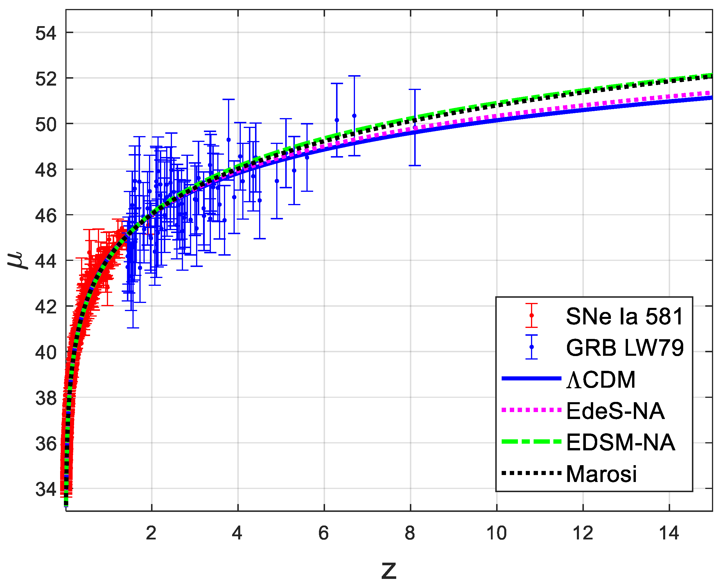
In this section we present the z − μ projections numerically in

Table 3. Calculated values of distance moduli versus redshift for the four selected models parameterized using the SNe Ia 580 dataset.

z	µ-ΛCDM	µ-EdeS-NA	µ-EDSM-NA	µ-Marosi	z	µ-ΛCDM	µ-EdeS-NA	µ-EDSM-NA	µ-Marosi
0.100	38.319	38.331	38.339	38.307	10.965	50.370	50.568	51.179	51.080
0.110	38.533	38.544	38.550	38.524	12.023	50.596	50.802	51.459	51.369
0.120	38.749	38.757	38.763	38.742	13.183	50.821	51.035	51.738	51.659
0.132	38.965	38.972	38.976	38.961	14.454	51.046	51.266	52.017	51.952
0.145	39.183	39.189	39.191	39.181	15.849	51.269	51.496	52.296	52.246
0.158	39.403	39.406	39.407	39.403	17.378	51.492	51.724	52.575	52.541
0.174	39.624	39.625	39.625	39.626	19.055	51.714	51.952	52.853	52.838
0.191	39.846	39.845	39.843	39.850	20.893	51.935	52.178	53.131	53.137
0.209	40.070	40.067	40.063	40.076	22.909	52.155	52.404	53.409	53.438
0.229	40.296	40.290	40.285	40.302	25.119	52.374	52.628	53.687	53.740
0.251	40.523	40.515	40.508	40.530	27.542	52.593	52.851	53.964	54.044
0.275	40.752	40.742	40.733	40.760	30.200	52.811	53.074	54.241	54.350
0.302	40.983	40.970	40.960	40.990	33.113	53.028	53.295	54.517	54.658
0.331	41.216	41.200	41.188	41.222	36.308	53.245	53.516	54.794	54.967
0.363	41.450	41.432	41.419	41.456	39.811	53.461	53.735	55.070	55.278
0.398	41.686	41.666	41.651	41.690	43.652	53.677	53.954	55.345	55.591
0.437	41.924	41.902	41.886	41.926	47.863	53.891	54.172	55.620	55.905
0.479	42.164	42.140	42.122	42.163	52.481	54.105	54.389	55.895	56.222
0.525	42.405	42.379	42.361	42.402	57.544	54.319	54.606	56.170	56.540
0.575	42.648	42.621	42.602	42.642	63.096	54.532	54.821	56.444	56.860
0.631	42.893	42.864	42.845	42.883	69.183	54.745	55.036	56.717	57.181
0.692	43.138	43.109	43.090	43.126	75.858	54.957	55.251	56.991	57.505
0.759	43.385	43.356	43.338	43.370	83.176	55.168	55.465	57.264	57.830
0.832	43.633	43.604	43.587	43.615	91.201	55.379	55.678	57.536	58.158
0.912	43.881	43.853	43.839	43.862	100.000	55.590	55.890	57.809	58.487
1.000	44.130	44.104	44.093	44.110	109.648	55.800	56.103	58.081	58.818
1.096	44.379	44.356	44.350	44.360	120.226	56.010	56.314	58.352	59.150
1.202	44.628	44.610	44.608	44.611	131.826	56.219	56.525	58.624	59.485
1.318	44.878	44.863	44.868	44.863	144.544	56.428	56.736	58.894	59.822
1.445	45.127	45.118	45.130	45.117	158.489	56.636	56.946	59.165	60.160
1.585	45.375	45.373	45.394	45.372	173.780	56.844	57.155	59.435	60.501
1.738	45.623	45.628	45.660	45.629	190.546	57.052	57.365	59.705	60.843
1.905	45.871	45.883	45.927	45.887	208.930	57.260	57.573	59.975	61.187
2.089	46.117	46.138	46.196	46.147	229.087	57.467	57.782	60.244	61.533
2.291	46.363	46.393	46.467	46.408	251.189	57.674	57.990	60.513	61.882
2.512	46.607	46.647	46.738	46.670	275.423	57.880	58.198	60.782	62.232
2.754	46.851	46.901	47.011	46.934	301.995	58.087	58.405	61.050	62.584
3.020	47.093	47.154	47.285	47.200	331.131	58.293	58.612	61.318	62.938
3.311	47.334	47.406	47.560	47.467	363.078	58.498	58.819	61.586	63.294
3.631	47.574	47.657	47.835	47.736	398.107	58.704	59.025	61.854	63.652
3.981	47.813	47.907	48.112	48.006	436.516	58.909	59.231	62.121	64.012
4.365	48.051	48.156	48.389	48.277	478.630	59.114	59.437	62.388	64.374
4.786	48.288	48.403	48.667	48.551	524.807	59.319	59.643	62.655	64.739
5.248	48.523	48.649	48.945	48.825	575.440	59.524	59.848	62.921	65.105
5.754	48.758	48.894	49.224	49.101	630.957	59.728	60.053	63.187	65.473
6.310	48.991	49.137	49.503	49.379	691.831	59.932	60.258	63.453	65.844
6.918	49.224	49.379	49.782	49.659	758.578	60.136	60.463	63.719	66.216
7.586	49.455	49.620	50.061	49.940	831.764	60.340	60.667	63.984	66.591
8.318	49.685	49.859	50.341	50.222	912.011	60.544	60.871	64.249	66.968
9.120	49.914	50.097	50.620	50.506	1000.000	60.747	61.076	64.514	67.347
10.000	50.142	50.333	50.900	50.792	1096.478	60.951	61.279	64.779	67.728

and graphically in Figure 1 using ΛCDM, EdeS-NA, EDSM-NA and Marosi models. In the figure, the lines indicate the four models constrained using the corresponding parameters in Table 1. SNe Ia data points (580 + 1) as well as the LW79 data points (79) have been shown with error bars in the figure. The redshift in the figure is up to z = 15 and in the table up to z = 1096. As the radiation density effects become significant for very high redshifts, extrapolating the models to such high values of the redshift may be considered academic. Nevertheless, the same is true for all the models and thus the comparison may still be meaningful. In addition, the radio telescope measurements of the redshift of the 21-cm (1420 MHz) hydrogen atom line at z ≥ 15 have started to be reported [7]. Radio astronomers can estimate the distances with some confidence using the graphs and tables produced here. Bowman et al. have recently reported observation of an absorption profile of this line centered at 78 MHz in the sky averaged spectrum [7]. This translates into z ≈ 17 spanning over 15 < z < 20. One could see from Table 3 that it corresponds to μ ≈ 51.5.

It should be mentioned that here we have considered only the redshift of the 21-cm absorption line. We do not consider in this paper the anomaly in the measured intensity of this line as it is a topic in itself and has been extensively discussed in literature since the publication of paper by Bowman et al. in Nature in 2018 [7], mostly on the ground that it might suggest new physics in cosmology. For example, Fraser et al. [34] propose soft photon emission by light dark matter as a natural solution to this anomaly; McGaugh [35] predicts that a universe devoid of cold dark matter will exhibit twice as much absorption as in the ΛCDM; Kovetz et al. [36] investigate the hypothesis that Coulomb-type interaction between dark matter and baryons to explain the anomaly; Xiao et al. [37] allow conformal and disformal coupling between dark matter and dark energy in a cosmological model to investigate the anomaly; Houston et al. [38] explain the anomaly using axions and axion like particles in the standard model, as they have the ability to mediate the required cooling process; Venumadhav et al. [39] show that HI spins and Lyman-α photons act as mediators between the radio background and the random thermal motions of the HI atoms, and hence cause extra heating of the intergalactic medium during cosmic dawn, causing higher than normal absorption; Lawson and Zhitnitsky [40] argue that dark matter in the form of macroscopically large nuggets of standard model quarks and antiquarks can explain the anomaly; Pospelov et al. [41] have suggested the enhancement of the Rayleigh-Jeans tail of the cosmic microwave background and show that the resonant oscillation of dark photons into regular photons in the redshift interval 20 < z < 1700 can be invoked as an explanation of the anomalous absorption; and D’Amico et al. [42] provide bounds on the dark-matter annihilations from the analysis of the 21-cm data.

We notice that the calculated distance modulus differences among the selected models for any particular redshift are way less than the μ error bars in the data. The difference in μ values between the ΛCDM model and the EdeS-NA model even at the highest redshift of 1096 in Table 3 is only 0.328. Until the error bars can be reduced significantly, it would be difficult to say which model or models should be rejected. One may wonder if the thirty meter telescope (TMT), due for commissioning in the year 2027, will be able to observe supernovae with high redshifts comparable to the highest GRB redshift with high enough precision to positively decide which model is better [33]!

7. Conclusions

The analysis of various models has shown that while most models can be made to fit the observed data rather satisfactorily with fairly high value of χ² probability, they tend to fizzle out when they are tested for their predictive power. We have used the redshift—distance modulus (z − μ) data for 580 supernovae Ia with 0.015 ≤ z ≤ 1.414 to determine the parameters for each model and then use the parameterized models to see how well each model fits the sole SNe Ia data at z = 1.914 and the GRB data up to z = 8.1. This essentially shows the predictive capability of a model parameterized with z ≤ 1.414 for data obtained at z > 1.414. We find that the standard ΛCDM model gives the highest χ² probability in all cases but one, albeit with a rather small margin over the next best model—the EdeS-NA model. We have made (z − μ) projections up to z = 1096 for the best four models just to show that how little the best two models, based on entirely different assumptions, differ even at such high redshift value which are indeed unmeasurable. The best two models differ in μ only by 0.328 at z = 1096, a tiny fraction of the measurement errors that are in the high redshift datasets. The third best model, the EDSM-NA model, has somewhat higher μ, with a difference of 3.828 at z = 1096, well within the expected measurement errors for such a high redshift objects. It appears unlikely that the measurement errors could be reduced to level where we could say for sure which model predicts the observations better. Other attributes of the model may then decide which model should be preferred.

The ΛCDM model is based on the ad hoc cosmological constant Λ introduced by Einstein in his field equations to prevent the universe from collapsing. There is no physics behind it, and it leads to energy entering the universe from nowhere to keep the energy density corresponding to Λ constant in time. In other words, the presence of Λ makes the universe implicitly nonadiabatic2. The EdeS-NA and EDSM-NA models are based on explicitly nonadiabatic assumption about the universe, that is, the energy leaves or enters a volume of the universe proportional to the energy contained in that volume [23]. This leads to time dependence of the nonadiabatic component of the energy density in an expanding or contracting universe when its energy density is changing. Another attribute of the EdeS-NA and EDSM-NA models is that they are parameterized by just one parameter, the Hubble constant. The second model parameter is not a fit parameter as it is determined analytically in the model. We therefore conclude that the EdeS-NA and EDSM-NA models are viable alternative to the ΛCDM model, even at very high redshift such as those encountered in radio astronomy.

References

- Zwicky, F. On the red shift of spectral lines through interstellar space. Proc. Natl Acad. Sci. USA 1929, 15, 773–779. [Google Scholar] [CrossRef]
- Penzias, A.A.; Wilson, R.W. A measurement of excess antenna temperature at 4080 Mc/s. Astrophys. J. 1965, 142, 419–421. [Google Scholar] [CrossRef]
- Marmet, L. On the Interpretation of Spectral Red-Shift in Astrophysics: A Survey of Red-Shift Mechanisms-II. arXiv 2018, arXiv:1801.07582. [Google Scholar]
- Vishwakarma, R.G.; Narlikar, J.V. Is it no longer necessary to test cosmologies with type Ia supernovae? Universe 2018, 4, 73. [Google Scholar] [CrossRef]
- Prichard, J.R.; Loeb, A. 21-cm cosmology. Rep. Prog. Phys. 2012, 75, 086901. [Google Scholar] [CrossRef] [PubMed]
- Boyarsky, A.; Lakubovskyi, D.; Ruchayskiy, O.; Rudakovskyi, A.; Valkenburg, W. 21-cm observation and warm dark matter models. arXiv 2019, arXiv:1904-03097. [Google Scholar]
- Bowman, J.D.; Rogers, A.E.E.; Mousalve, R.A.; Mozdzen, T.J.; Mahesh, N. An absorption profile centred at 78 MHz in the sky-averaged spectrum. Nature 2018, 555, 67–70. [Google Scholar] [CrossRef]
- López-Corredoira, M. Test and problems of the standard model in cosmology. Found. Phys. 2017, 47, 711–768. [Google Scholar] [CrossRef]
- Orlov, V.V.; Raikov, A.A. Cosmological tests and evolution of extragalactic objects. Astron. Rep. 2016, 60, 477–485. [Google Scholar] [CrossRef]
- Berton, G.; Hooper, D. Particle dark matter: Evidence. Phys. Rept. 2005, 405, 279–390. [Google Scholar] [CrossRef]
- Del Popolo, A. Nonbaryonic dark matter in cosmology. Int. J. Mod. Phys. D 2014, 23, 1430005. [Google Scholar] [CrossRef]
- Del Popolo, A.; Le Delliou, M. Small scale problems of the ΛCDM model: A short review. Galaxies 2017, 5, 17. [Google Scholar] [CrossRef]
- Mortonson, M.J.; Weinberg, D.H.; While, M. Dark energy: A short review. arXiv 2013, arXiv:1401.0046. [Google Scholar]
- Ryden, B. Introduction to Cosmology; Cambridge University Press: Cambridge, UK, 2017. [Google Scholar]
- Gupta, R.P. Mass of the universe and the redshift. Int. J. Astron. Astrophys. 2018, 8, 68–78. [Google Scholar] [CrossRef]
- Gupta, R.P. Static and dynamic components of the redshift. Int. J. Astron. Astrophys. 2018, 8, 219–229. [Google Scholar] [CrossRef]
- Crawford, D. A problem with the analysis of type Ia Supernovae. Open Astron. 2017, 26, 111–119. [Google Scholar] [CrossRef]
- Marosi, L.A. Hubble diagram test of 280 supernovae redshift data. J. Mod. Phys. 2014, 5, 29–33. [Google Scholar] [CrossRef]
- Vishwakarma, R.G. A scale-invariant, Machian theory of gravitation and electrodynamics unified. Int. J. Geom. Meth. Mod. Phys. 2018, 15, 1850178. [Google Scholar] [CrossRef]
- Zaninetti, L. On the number of galaxies at high redshift. Galaxie 2015, 3, 129–155. [Google Scholar] [CrossRef]
- Zaninetti, L. Padé Approximant and Minimax Rational Approximation in Standard Cosmology. Galaxies 2016, 4, 4–24. [Google Scholar] [CrossRef]
- Brynjolfsson, A. Redshift of photons penetrating a hot plasma. arXiv 2004, arXiv:astro-ph/0401420. [Google Scholar]
- Gupta, R.P. SNe Ia redshift in a nonadiabatic universe. Universe 2018, 4, 104. [Google Scholar] [CrossRef]
- Peebles, P.J.E. Principles of Physical Cosmology; Princeton University Press: Princeton, NJ, USA, 1993. [Google Scholar]
- Press, W.H.; Teukolsky, S.A.; Vetterling, W.T.; Flannery, B.P. Numerical Recipes in C—The Art of Scientific Computing, 2nd ed.; Cambridge University Press: Cambridge, UK, 1992. [Google Scholar]
- Walker, J. Chi-Square Calculator. 2018. Available online: https: //www.fourmilab.ch/rpkp/experiments/analysis/chiCalc.html (accessed on 30 April 2019).
- Amanullah, R.; Lidman, C.; Rubin, D.; Aldering, G.; Astier, P.; Barbary, K.; Burns, M.S.; Conley, A.; Dawson, K.S.; Deustua, S.E.; et al. Spectra and Hubble space telescope light curves of six type Ia supernovae at 0.511 < z < 1.12 and the UNION2 Compilation. Astrophys. J. 2010, 716, 712–738. [Google Scholar]
- Jones, D.O.; Rodney, S.A.; Riess, A.G.; Mobasher, B.; Dahlen, T.; McCully, C.; Frederiksen, T.F.; Casertano, S.; Hjorth, J.; Keeton, C.R.; et al. The discovery of the most distant known Type Ia supernova at redshift 1.914. Astrophys. J. 2013, 768, 166. [Google Scholar] [CrossRef]
- Liu, J.; Wei, H. Cosmological models and gamma-ray bursts calibrated by using Padé method. Gen. Relativ. Gravit. 2015, 47, 141. [Google Scholar] [CrossRef]
- Cardone, V.F.; Capozziello, S.; Dainotti, M.G. An updated gamma-ray bursts Hubble Diagram. Mon. Not. R. Astron. Soc. 2009, 400, 775–790. [Google Scholar] [CrossRef]
- Liang, N.; Zhang, S.N. Cosmology-independent distance moduli of 42 gamma-ray bursts between redshift of 1.44 and 6.60. AIP Conf. Proc. 2008, 1065, 367. [Google Scholar]
- Lin, H.-N.; Li, X.; Chang, Z. Model independent distance calibration of high-redshift gamma-ray bursts and constrain on ΛCDM model. Mon. Not. R. Astron. Soc. 2016, 455, 2131–2138. [Google Scholar] [CrossRef]
- Pandey, S.B. Core-collapse supernovae and gamma-ray bursts in TMT era. J. Astrophys. Astron. 2013, 34, 157–173. [Google Scholar] [CrossRef]
- Fraser, S.; Hector, A.; Hutsi, G.; Kannike, K.; Marzo, C.; Marzola, L.; Racioppi, A.; Raidal, M.; Spethmann, C.; Vaskonen, V.; et al. The EDGES 21 cm Anomaly and Properties of Dark Matter. Phys. Letts. B 2018, 785, 159–164. [Google Scholar] [CrossRef]
- McGaugh, S.S. Predictions for the sky averaged depth of the 21 cm absorption signal at high redshift in cosmologies with and without nonbaryonic cold dark matter. Phys. Rev. Lett. 2018, 121, 081305. [Google Scholar] [CrossRef]
- Kovetz, E.D.; Poulin, V.; Gluscevic, V.; Boddy, K.K.; Barkana, R.; Kamionkowski, M. Tighter limits on dark matter explanations on the anomalous EDGES 21 cm signal. Phys. Rev. D 2018, 98, 103529. [Google Scholar] [CrossRef]
- Xiao, L.; An, R.; Zhang, L.; Yue, B.; Xu, Y.; Wang, B. Can conformal and disformal coupling between dark sectors explain the EDGES 21-cm anomaly? Phys. Rev. D 2018, 99, 023528. [Google Scholar] [CrossRef]
- Houston, N.; Li, C.; Li, T.; Yang, Q.; Zhang, X. Natural explanation for 21 cam absorption signal via axion-induced cooling. Phys. Rev. Lett. 2018, 121, 111301. [Google Scholar] [CrossRef]
- Venumadhav, T.; Dai, L.; Kaurov, A.; Zaldarriaga, M. Heating of the intergalactic medium by the cosmic microwave background during cosmic dawn. Phys. Rev. D 2018, 98, 103513. [Google Scholar] [CrossRef]
- Lawson, K.; Zhitnitsky, A.R. The 21 cm absorption line and the axion quark nugget dark matter model. Phys. Dark Universe 2018, 24, 100295. [Google Scholar] [CrossRef]
- Pospelov, M.; Pradler, J.; Ruderman, J.T.; Urbano, A. Room for new physics in the Rayleigh-Jeans tail of the cosmic microwave background. Phys. Rev. Lett. 2018, 121, 031103. [Google Scholar] [CrossRef]
- D’Amico, G.; Panci, P.; Strumia, A. Bounds on dark-matter annihilation from 21-cm data. Phys. Rev. Lett. 2018, 121, 011103. [Google Scholar] [CrossRef]