Abstract
For the accretion flow in extremely low-luminosity active galactic nuclei, such as our Galactic center (Sgr A*) and M 87, the collisional mean-free path of ions may be much larger than its gyroradius. In this case, the pressure parallel to the magnetic field is different from that perpendicular to the field; therefore, the pressure is anisotropic. We study the effects of anisotropic pressure on the dynamics of accretion flow by assuming the flow is radially self-similar. We find that in the case where the outflow is present, the radial and rotational velocities, the sound speed, and the Bernoulli parameter of the accretion flow are all increased when the anisotropic pressure is taken into account. This result suggests that it becomes easier for the accretion flow to generate outflow in the presence of anisotropic pressure.
1. Introduction
According to the temperature of the gas, black hole accretion disk/flow can be divided into two groups, namely cold accretion disk and hot accretion flow. There are many numerical simulations studying thin disks. One of the hot topics being studied by simulations is jet launching from a thin disk (e.g., Casse and Keppens [1,2]; Zanni et al. [3,4]; Sheikhnezami et al. [5]; Sheikhnezami and Fendt [6,7]). The acceleration of jets from a thin disk is also being studied by analytical works (e.g., Takahashi et al. [8]). Simulations also studied relativistic thin disks (e.g., De Villiers and Hawley [9,10]; Gammie et al. [11]; Noble et al. [12]; Sadowski et al. [13]). Hawley et al. [14] gave a very extensive review for accretion disks.
Observations show that most of the galactic nuclei in the local universe are very dim (Ho [15] and the references therein). Radiatively inefficient hot accretion flows operate in these sources (Narayan and Yi [16]; see the reviews by Ho [15] and Yuan and Narayan [17]). Hot accretion flows also operate in the quiescent and hard states of black hole X-ray binaries (Done et al. [18]; Qiao and Liu [19]; Gilfanov [20]; Zhang et al. [21]; Yan and Yu [22]; see the review by Yuan and Narayan [17]). The temperature of the gas in the hot accretion flow almost equals the virial temperature. In the innermost region, the gas can have a temperature of approximately K (Yuan and Narayan [17]). The density is very low and depends on the mass accretion rate. In the accretion flow in the Galactic center, in the innermost region, gas density is approximately .
Recently, numerical simulations found that strong outflow can be launched in hot accretion flows (e.g., Yuan et al. [23,24]; Narayan et al. [25]; Li et al. [26]; Bu et al. [27]; Bu et al. [28,29]). The properties of outflow from hot accretion flows have also been studied by analytical works (Xue and Wang [30]; Akizuki and Fukue [31]; Bu et al. [32]; Li and Cao [33]; Jiao and Wu [34]; Begelman [35]; Wu et al. [36]; Gu [37]; Cao [38]; Ghasemnezhad and Abbassi [39]; Kumar and Gu [40]). Observations of low-luminosity active galactic nuclei and a hard state of black hole X-ray binaries showed indirect evidence that strong outflow can be launched in hot accretion flows (e.g., Crenshaw and Kraemer [41]; Cheung et al. [42]; Homan et al. [43]; Ma et al. [44]; Park et al. [45]). Outflows can interact with the interstellar medium surrounding the active galactic nuclei (AGNs). Outflows can push away the gas surrounding the AGN, which will decrease the black hole accretion rate and affect the star formation rate (Ostriker et al. [46]; Ciotti et al. [47,48]; Weinberger et al. [49,50]; Yuan et al. [51]; Yoon et al. [52]; Bu and Yang [53]).
There are some extremely low accretion rate accretion flows. For example, the accretion rate of the accretion flow in the Galactic center (Sgr A*) is , with and c being the Eddington luminosity and the speed of light, respectively. The other example is the accretion flow in the M87 galaxy. The accretion rate of the accretion flow in M87 is (Yuan and Narayan [17]). In these extremely low accretion rate hot accretion flows, such as the accretion flow in the Galactic center (Sgr A*) and M87, the Coulomb collision mean free paths of both electrons and ions are much larger than the typical length-scale of the accretion flows, ∼GM/c, where G and M are the gravitational constant and black hole mass, respectively (Tanaka and Menou [54]; Johnson and Quataert [55]; Foucart et al. [56]). At first glance, magneto-hydrodynamic (MHD) approximations cannot be applied to these plasmas, and we should solve the distribution function of both ions and electrons. However, particle-in-cell simulations show that the wave–particle interactions can effectively increase the collision rate between particles (Kunz, Schekochihin, and Stone [57]; Riquelme, Quataert, and Verscharen [58]; Sironi and Narayan [59]). The plasmas in these extreme low accretion rate accretion flows are just weakly collisional. For the weakly-collisional plasmas, the non-ideal effects can be treated as perturbations relative to an ideal fluid, by the inclusion of anisotropic thermal conduction and anisotropic pressure (Foucart et al. [56]).
In weakly-collisional accretion flows, anisotropic thermal conduction is important and along the magnetic field lines (Parrish and Stone [60]; Sharma, Quataert, and Stone [61]; Bu, Yuan and Stone [62]). Thermal conduction can transport thermal energy from the inner (hotter) to the outer (cooler) regions. Previous works showed that at large radii, the gas temperature can be increased to be above the virial temperature. Strong outflows can be launched, and the black hole mass accretion rate can be significantly decreased (Bu et al. [63]).
As introduced above, in weakly-collisional accretion flows, one should include an anisotropic pressure as perturbations to an ideal fluid. In weakly-collisional accretion flows, the ions collision mean free path can be much larger than its gyroradius. For example, the ions’ mean free path in the accretion flow in the Galactic center (Sgr A*) is ∼10 (Tanaka and Menou [54]). If we assume that magnetic pressure is 0.1-times the gas pressure, we will have that ions gyro-radius is ∼4 (Bu et al. [63]). In these systems, pressure parallel to the magnetic field is different from that perpendicular to the magnetic field (Quataert et al. [64]; Sharma et al. [65]; Chandra et al. [66]). The pressure anisotropy can be modeled by an anisotropic viscosity with respect to magnetic field lines (Balbus [67]; Islam and Balbus [68]). In Wu et al. [69], the effects of anisotropic pressure on properties of hot accretion flows were studied. We note that in that paper, only a very weak magnetic field was considered, and the magnetic pressure was at least four orders of magnitude smaller than the gas pressure. They found that when magnetic fields are extremely weak, Maxwell stress is negligibly small. Anisotropic pressure can transfer angular momentum, and a hot accretion flow can be formed. Furthermore, they found very weak outflow.
Currently, it is quite difficult to measure or even to constrain the strength of the magnetic field. Among the existing methods, the Faraday rotation measure (RM) can provide the integration of electron density and magnetic field along the line of sight. RM combined with spectrum can roughly give magnetic field strength. For example, the RM of Sgr A*, together with the radio-up to-millimeter spectrum, constrains the magnetic field strength in the accretion flow to be 20 Gauss at 10 Schwarzschild radii (Yuan et al. [70]).
The magnetic stress for angular momentum transfer is induced by turbulence driven by magnetorotational instability (Balbus and Hawley [71,72]). The stress is , with and being the radial and toroidal components of the magnetic field, respectively. The viscous coefficient () is stress divided by gas pressure. Therefore, we have , with p and B being the gas pressure and magnetic field, respectively. Observations of some accretion systems indicate that the viscosity coefficient (see King et al. [73] and the references in that paper). Since , such a value of implies that the magnetic pressure is approximately -times the gas pressure. The magnetic field is not significantly weak compared to the gas pressure. The effects of anisotropic pressure in hot accretion flows with a relatively strong magnetic field have not been studied previously. In this work, we study the effects of pressure anisotropy (or anisotropic viscosity) on the properties of hot accretion flows in this case. We set the magnetic pressure to be 0.1-times the gas pressure.
2. Basic Equations and Assumptions
We study time-steady and axisymmetric () accretion flows in cylindrical coordinates (). The basic equations describing accretion are as follows,
In the equations, is the gas density, is velocity, e is gas specific internal energy, is the gravitational potential, is the heating rate of the gas, and represents the radiative cooling rate. For hot accretion flows, the radiative cooling is not important. For simplicity, we assume that and . In this paper, we use the Newtonian potential. .
Numerical simulations found that the magnetic field in an accretion flow/disk can be decomposed into a large-scale ordered component and a turbulent component (e.g., Machida et al. [74]; Hirose et al. [75]; Bai and Stone [76]). In Equation (2), we use B to represent the large-scale ordered magnetic field component. Simulations showed that the main body of the accretion flow is governed by a toroidal magnetic field (see Figure 6 in Hirose et al. [75]). In this paper, we assume that the large-scale ordered magnetic field has only the toroidal component (). Following Lovelace et al. [77], we assume that is an odd function of z.
H is the half-thickness of the accretion flow. The large-scale magnetic field only has a toroidal component, and we assume axisymmetry; therefore, the divergence-free condition of the magnetic field is satisfied. We note that for the strongly-magnetized accretion flow (MAD disk, Narayan et al. [25]), a substantial poloidal field is present. We plan to study accretion flow with the poloidal magnetic field in the future.
In Equation (2), the term represents the angular momentum transfer by the turbulent magnetic field component. For the stress T, we use the usual description,
In this equation, . is sound speed; is the Keplerian angular velocity; is the angular velocity of the gas. Numerical simulations showed that the dissipation heating mainly comes from the magnetic reconnection associated with the turbulent magnetic field (Hirose et al. [78]). In Equation (4), we use to represent the heating due to the magnetic reconnection due to the turbulent component of the magnetic field.
Following Chandra et al. [66], we use anisotropic viscous stress tensor to model the effects of ion pressure anisotropy (see also Braginskii [79]),
where is the unit vector in magnetic field direction, and is the unit tensor. is a dyadic tensor defined as,
and
In Equation (8),
We use to denote the strength of anisotropic pressure. In this paper, the magnetic field only has a toroidal component. Correspondingly, the anisotropic pressure only has three non-zero components,
In Equation (4), the term represents the heating by the work done by anisotropic pressure.
2.1. Vertical Integrated Equations
In this paper, we use several parameters (, , ; see the definitions below) to characterize the properties of outflows. We assume that the z component of gas velocity is zero. We also assume that the gas is vertically isothermal. The temperature or sound speed is only a function of r. At a fixed radius, the gas temperature or sound speed does not change with height. We vertically integrate Equations (1)–(3) to obtain one-dimensional equations. In the presence of outflow, the vertically-integrated mass conservation Equation (1) will be as follows,
is constant. The parameter s is in the range (see the explanation below).
In the presence of outflow, the equations describing inflow are given in Xie and Yuan [80]. The radial momentum equation is,
In this equation, is the surface density and defined as . In Equation (13), is the radial velocity of outflow. When the radial velocity of outflow is different from that of inflow, radial momentum will be taken away from or deposited into inflow by the outflow. Correspondingly, the inflow velocity will be changed. The first, second, and third terms on the right-hand side of Equation (13) are centrifugal, gravitational, and gas pressure gradient forces, respectively. The fourth term is the Lorentz force due to the large-scale ordered magnetic field. The last two terms are the forces of divergence of anisotropic pressure ( in Equation (2)).
The azimuthal momentum equation is,
In this equation, is the Keplerian rotational velocity. is the rotational velocity of outflow. If the rotational velocity of outflow is different from that of inflow, angular momentum will be taken away from or deposited into the inflow by the outflow. Correspondingly, the angular momentum of inflow will be changed. The term on the right-hand side is the angular momentum transfer by the turbulent magnetic field ( in Equation (2)).
We define a parameter to describe the strength of the large-scale ordered magnetic field,
The gas in the vertical direction achieves static equilibrium, and the -component of gravitational force is balanced by gas pressure gradient and magnetic pressure gradient forces,
We note that the force of divergence of anisotropic pressure ( in Equation (2)) only exists in the radial momentum equation. This is because the anisotropic pressure only has the , , components. Anisotropic pressure cannot transfer angular momentum, because its component is zero.
The energy equation is,
is the ratio of the specific heats, which varies from the relativistic value to the typical monatomic gas value . In this paper, we set . We find that the results are not sensitive to the value of . is the specific internal energy of outflow. If the specific internal energy of outflow is different from that of inflow, internal energy will be taken away from or deposited into the inflow by the outflow. Correspondingly, the internal energy of inflow will be changed. The first term on the right-hand side is the heating due to the reconnection of turbulent magnetic field ( in Equation (4)). The second term on the right-hand side is the heating due to the work done by anisotropic pressure ( in Equation (4)).
We parameterize the outflow properties. We assume that the velocities of outflow are proportional to those of inflow, with and . The specific internal energy of outflow is proportional to that of inflow, with .
2.2. Self-Similar Assumptions
Following Narayan and Yi [16], we set the following radially self-similar assumptions,
The radial velocity . The mass accretion rate . If outflow is absent, the mass accretion rate will be a constant with radius, and we will have . When outflow is present, the mass accretion rate will decrease with decreasing radius. Numerical simulations found that when outflow is present, the density profile is very shallow , with (Stone et al. [81]). The surface density . For hot accretion flows, the scale height of the flow is roughly equal to the radius . Therefore, we have . is a constant. The parameter is in the range . corresponds to the case where outflow is absent.
Using Equation (18), the momentum Equations (13) and (14), and the vertical static equilibrium Equation (16) reduce to,
The energy Equation (17) becomes,
3. Results
In this paper, we set and . We focused on studying the effects of anisotropic pressure. For a hot accretion flow, the gas temperature was too high such that gas was fully ionized. Observationally, it is very hard to detect outflow directly through the absorption line. There is only some indirect evidence that outflow should be present for a hot accretion flow (Wang et al. [82]; Ma et al. [44]; Park et al. [45]). The properties (velocity, temperature) of outflows cannot be given by observations. Numerical simulations give us the properties of outflows. The values of were mainly from numerical simulations’ results (Yuan et al. [23]).
3.1. Accretion Flow without Outflow
In this subsection, we focus on the case where outflows are absent. In this case, the parameter . We show the results in Figure 1. The top-left panel plots radial infall velocity (in units of Keplerian velocity) as a function of the strength of anisotropic pressure (). The top-right panel plots rotational velocity (in units of Keplerian velocity) as a function of the strength of anisotropic pressure (). The lower panel plots sound speed (in units of Keplerian velocity) as a function of the strength of anisotropic pressure (). The viscous coefficient was set to be 0.1. The ratio of magnetic to gas pressure was set to be 0.1. For the self-similar solution, at any radii, the ratio of velocities to Keplerian velocity was constant. In the figure, we plot the ratio of velocities to Keplerian velocity; therefore, the results (velocities plotted in the top-left panel of Figure 1) can be applied at any radii.
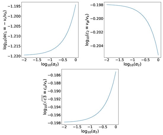
Figure 1.
The properties of the accretion flow when outflow is absent (). The top-left panel plots radial infall velocity (in units of Keplerian velocity) as a function of the strength of anisotropic pressure (). The top-right panel plots rotational velocity (in units of Keplerian velocity) as a function of the strength of anisotropic pressure (). The lower panel plots sound speed (in units of Keplerian velocity) as a function of the strength of anisotropic pressure (). The viscous coefficient was set to be 0.1. The ratio of magnetic to gas pressure was set to be 0.1.
The last term on the right-hand side of the radial momentum Equation (19) is the force of divergence of anisotropic pressure. It is clear, when , that the force is negative; this force points towards the central black hole. Therefore, from the top-left panel of Figure 1, we see that with the increase of strength of anisotropic pressure, the radial infall velocity of the accretion flow increases. If outflow is absent, viscosity due to turbulent magnetic field is the only mechanism for angular momentum transfer (see Equations (14) and (20)). The inward advection of angular momentum by inflowing gas is balanced by the outward angular momentum transportation by viscosity. With the increase of radial infall velocity, the inward advection of angular momentum flux increases (see Equation (20)). Correspondingly, the outward angular momentum flux also needs to increase. The increase of outward angular momentum flux can be realized by increasing the sound speed (see Equation (20)), because the viscosity T is proportional to . Therefore, with the increase of strength of anisotropic pressure, the sound speed (or gas temperature) becomes bigger. From the energy Equation (22), we see that the viscous heating (first term on the right-hand side) and heating due to work done by anisotropic pressure (second term on the right-hand side) are balanced by the advection of energy by the inflow (first term on the left-hand side). With the increase of , heating due to work done by anisotropic pressure increases faster than the increase of energy advection. Therefore, in order to keep the accretion flow stable, the viscous heating term needs to decrease with an increase of . Therefore, with an increase of , the rotational velocity decreases.
From Figure 1, we see that with the increase of , both the radial infall velocity and sound speed increase. Comparing the top-left and lower panels, we see that the infall velocity is always smaller than the sound speed by one order of magnitude at any given value of . Therefore, the infall velocity is sub-sonic. We assume that magnetic pressure is 10-times smaller than gas pressure. Correspondingly, the Alfvenic velocity is smaller than gas sound speed by a factor of 3.3. Therefore, the gas infall velocity is sub-Alfvenic.
3.2. Accretion Flow with Outflow
We first studied the case where the specific velocity and internal energy of outflow are the same as those of inflow (). The results are shown by the blue lines in Figure 2. With the increase of strength of anisotropic pressure (), the infall velocity () increases. The reason is the same as explained for the case where the outflow is absent. The force of the anisotropic pressure gradient is negative. Therefore, with an increase of , gas infall velocity increases. With the increase of infall velocity (), the sound speed increases. The reason is also the same as in the case where the outflow is absent, as introduced in the last subsection. We do not explain it again here. We now explain why the rotational velocity increases with an increase of . As introduced above, the viscous heating and heating due to work done by anisotropic pressure are balanced by the advection of energy by the inflow (see Equations (17) and (22)). With the increase of , the energy advection term increases faster than the increase of work done by anisotropic pressure. Therefore, in order to keep the accretion flow stable, the viscous heating term needs to increase with an increase of . Therefore, with an increase of , the rotational velocity increases.
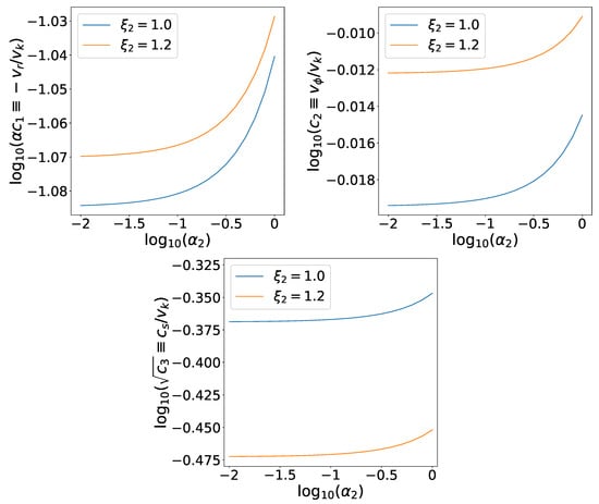
Figure 2.
The properties of the accretion flow when outflow is present (). The top-left panel plots radial infall velocity (in units of Keplerian velocity) as a function of the strength of anisotropic pressure (). The top-right panel plots rotational velocity (in units of Keplerian velocity) as a function of the strength of anisotropic pressure (). The lower panel plots sound speed (in units of Keplerian velocity) as a function of the strength of anisotropic pressure (). The viscous coefficient was set to be 0.1. The ratio of magnetic to gas pressure was set to be 0.1. is the ratio of outflow radial velocity to inflow radial velocity. is the ratio of outflow rotational velocity to inflow rotational velocity. is the ratio of outflow sound speed to inflow sound speed. We set . The blue and yellow lines correspond to and , respectively.
Now, we study the cases where the specific velocity and internal energy of outflow are different from those of inflow. We first study the effects of the discrepancy of the radial velocity between inflow and outflow. We find that for a reasonable change of values of , the effects are of minor importance. This result is consistent with Xie and Yuan [80]. Therefore, for the models described below, we set .
MHD numerical simulation by Yuan et al. [23] has found that the specific angular momentum of outflow is higher than that of inflow. We study the case where the specific angular momentum of outflow is higher than that of inflow by setting . The results are shown in Figure 2 by the yellow lines. We first focus on the angular momentum Equation (20). In this equation, as introduced above, the first term on the left-hand side is the angular momentum advection by inflow gas. The second term on the left-hand side is the angular momentum flux taken away by outflow. The term on the right-hand side corresponds to the angular momentum outward transportation by viscosity. The inward advection of angular momentum by gas inflow is balanced by the outward transportation of angular momentum by both outflow and viscosity. In the model with , outflow can take away angular momentum, so the outward flux of angular momentum transported by viscosity (denoted by sound speed in Equation (20)) becomes smaller. Therefore, with the same value of , the sound speed in model is smaller than that in the model . With the help of outflow (), the total outward transportation rate of angular momentum by both outflow and viscosity is larger than that in the case . Therefore, the inward advection term of angular momentum (denoted by radial velocity in Equation (20)) in the model with should be larger than that in the model with . Therefore, with the same value of , the radial velocity in the model with is larger than that in the model with . From the energy Equation (22), with an increase of , the energy advection term increases faster than the increase of work done by anisotropic pressure. Therefore, in order to keep the accretion flow stable, the viscous heating term (denoted by ) needs to increase with an increase of . Therefore, with the same value of , in the model with is larger than that in the model with .
The specific internal energy of outflow was also found to be higher than that of inflow by simulations (e.g., Yuan et al. [23]). In Figure 3, we show the results for the flow in which outflow specific internal energy is higher than that of inflow by the yellow lines. When we calculated the results shown by yellow lines, we set . Note that the results shown by blue lines in this figure were calculated with . They are the same as the results shown by blue lines in Figure 2. Now, we see the energy Equation (22). The first term on the left-hand side is the advection of energy by gas inflow. The second term on the left-hand side is the energy taken away by outflow. The two terms on the right-hand side are heating by viscosity and work done by anisotropic pressure. One portion of the heating energy is advected to the black hole by gas inflow; the other portion is taken away by outflow. In the model with , the energy can be taken away by outflow; therefore, the energy advection term (denoted by ) becomes smaller. Therefore, with the same value of , the radial velocity of inflow () in the model with is smaller than that in the model with . From the angular momentum Equation (20), we see that with the decrease of , the sound speed also decreases. Therefore, with the same value of , the sound speed () in the model with is smaller than that in the model with . With the decrease of sound speed, gas pressure gradient force in the radial direction decreases. In order to keep a balance of the forces in the radial direction, the centrifugal force should increase. Therefore, with the same value of , the value of in the model with is bigger than that in the model with .
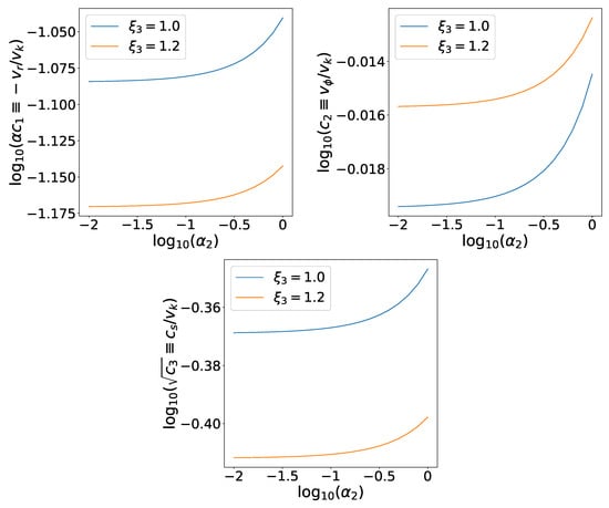
Figure 3.
The properties of the accretion flow when outflow is present (). The top-left panel plots radial infall velocity (in units of Keplerian velocity) as a function of the strength of anisotropic pressure (). The top-right panel plots rotational velocity (in units of Keplerian velocity) as a function of the strength of anisotropic pressure (). The lower panel plots sound speed (in units of Keplerian velocity) as a function of the strength of anisotropic pressure (). The viscous coefficient was set to be 0.1. The ratio of magnetic to gas pressure was set to be 0.1. is the ratio of outflow radial velocity to inflow radial velocity. is the ratio of outflow rotational velocity to inflow rotational velocity. is the ratio of outflow sound speed to inflow sound speed. We set . The blue and yellow lines correspond to and , respectively.
The Bernoulli parameter is usually used to judge whether outflow can escape from the black hole gravitational potential to infinity. In the magnetized accretion flow with only a toroidal magnetic field, the Bernoulli parameter is defined as,
Here, is enthalpy. Both the velocity and gas temperature increase with the increase of the strength of anisotropic pressure (). Therefore, the Bernoulli parameter increases with . The result indicates that the presence of anisotropic pressure makes it easier to generate outflow.
4. Conclusions
For an extremely low-accretion rate system, the ion’s mean-free path can be much larger than its gyroradius, and pressure parallel to the magnetic field is different from that perpendicular to the magnetic field. In this paper, we study the effects of anisotropic pressure on the dynamics of hot accretion flows. We find that when outflow is absent, the radial velocity and sound speed increase with the increase of the strength of anisotropic pressure, the rotational velocity decreases with the increase of the strength of anisotropic pressure. When outflow is present, the radial velocity, rotational velocity, and sound speed increase with the increase of strength of anisotropic pressure. Therefore, in this case, the Bernoulli parameter of the accretion flow increases. This result predicts that when anisotropic pressure is considered, it becomes easier to generate outflow by hot accretion flows.
Author Contributions
D.-F.B. is the corresponding author, who supplies the idea of this paper. P.-Y.X. is responsible for the calculations and plotting figures. B.-C.Z. discusses the physics with D.-F.B. and P.-Y.X.
Funding
This work is supported in part by the Natural Science Foundation of China (Grants 11773053, 11573051, 11633006, and 11661161012), the Natural Science Foundation of Shanghai (Grant 16ZR1442200), and the Key Research Program of Frontier Sciences of CAS(No. QYZDJSSW- SYS008).
Acknowledgments
This work made use of the High Performance Computing Resource at the Core Facility for Advanced Research Computing at Shanghai Astronomical Observatory.
Conflicts of Interest
The authors declare no conflict of interest. The funders had no role in the design of the study; in the collection, analyses, or interpretation of data; in the writing of the manuscript, or in the decision to publish the results.
References
- Casse, F.; Keppens, R. Magnetized Accretion-Ejection Structures: 2.5-dimensional Magnetohydrodynamic Simulations of Continuous Ideal Jet Launching from Resistive Accretion Disks. Astrophys. J. 2002, 581, 998–1001. [Google Scholar] [CrossRef]
- Casse, F.; Keppens, R. Radiatively Inefficient Magnetohydrodynamic Accretion-Ejection Structures. Astrophys. J. 2004, 601, 90. [Google Scholar] [CrossRef]
- Zanni, C.; Ferrari, A.; Massaglia, S.; Bodo, G.; Rossi, P. Launching jets from resistive accretion disks. Mem della Soc. Astron. Italiana 2005, 76, 372. [Google Scholar]
- Zanni, C.; Ferrari, A. MHD simulations of jet acceleration from Keplerian accretion disks. The effects of disk resistivity. Astron. Astrophys. 2007, 469, 811. [Google Scholar] [CrossRef]
- Sheikhnezami, S.; Fendt, C.; Porth, O.; Vaidya, B.; Ghanbari, J. Bipolar Jets Launched from Magnetically Diffusive Accretion Disks. I. Ejection Efficiency versus Field Strength and Diffusivity. Astrophys. J. 2012, 757, 65. [Google Scholar] [CrossRef]
- Sheikhnezami, S.; Fendt, C. MHD simulations of jet-launching from diffusive magnetized accretion disks. Eur. Conf. Lab. Astrophys. 2012, 58, 113–116. [Google Scholar] [CrossRef][Green Version]
- Sheikhnezami, S.; Fendt, C. Long-term Simulation of MHD Jet Launching in an Orbiting Star-Disk System. Astrophys. J. 2018, 861, 11. [Google Scholar] [CrossRef]
- Takahashi, M.; Nitta, S.; Yoshinori, T.; Akira, T. Magnetohydrodynamic flows in Kerr geometry—Energy extraction from black holes. Astrophys. J. 1990, 363, 206–217. [Google Scholar] [CrossRef]
- De Villiers, J.P.; Hawley, J.F. Three-dimensional Hydrodynamic Simulations of Accretion Tori in Kerr Spacetimes. Astrophys. J. 2002, 577, 866. [Google Scholar] [CrossRef]
- De Villiers, J.P.; Hawley, J.F. A Numerical Method for General Relativistic Magnetohydrodynamics. Astrophys. J. 2003, 589, 458. [Google Scholar] [CrossRef]
- Gammie, C.F.; McKinney, J.C. Tóth, G. HARM: A Numerical Scheme for General Relativistic Magnetohydrodynamics. Astrophys. J. 2003, 589, 444. [Google Scholar] [CrossRef]
- Noble, S.C.; Krolik, J.H.; Schnittman, J.D.; Hawley, J.F. Radiative Efficiency and Thermal Spectrum of Accretion onto Schwarzschild Black Holes. Astrophys. J. 2011, 743, 115. [Google Scholar] [CrossRef]
- Sądowski, A.; Abramowicz, M.; Bursa, M.; Kluzniak, W.; Lasota, J.; Rozanska, A. Relativistic slim disks with vertical structure. Astron. Astrophys. 2011, 527, 17. [Google Scholar] [CrossRef]
- Hawley, J.F.; Fendt, C.; Hardcastle, M.; Nokhrina, E.; Tchekhovskoy, A. Disks and Jets. Gravity, Rotation and Magnetic Fields. Space Sci. Rev. 2015, 191, 441. [Google Scholar] [CrossRef]
- Ho, L. Nuclear activity in nearby galaxies. Annu. Rev. Astron. Astrophys. 2008, 46, 475–539. [Google Scholar] [CrossRef]
- Narayan, R.; Yi, I. Advection-dominated accretion: A self-similar solution. Astrophys. J. 1994, 428, L13. [Google Scholar] [CrossRef]
- Yuan, F.; Narayan, R. Hot accretion flows around black holes. Ann. Rev. Astron. Astrophys. 2014, 52, 529. [Google Scholar] [CrossRef]
- Done, C.; Gierliński, M.; Kubota, A. Modelling the behaviour of accretion flows in X-ray binaries. Everything you always wanted to know about accretion but were afraid to ask. Astron. Astrophys. Rev. 2007, 15, 1–66. [Google Scholar] [CrossRef]
- Qiao, E.; Liu, B. Dependence of spectral state transition and disk truncation on viscosity parameter alpha. Publ. Astron. Soc. Jpn. 2009, 61, 403–410. [Google Scholar] [CrossRef]
- Gilfanov, M. X-ray Emission from Black-Hole Binaries. In Lecture Notes in Physics; The Jet Paradigm-From Microquasars to Quasars; Belloni, T., Ed.; Springer: Berlin, Germany, 2010; Volume 794, p. 17. [Google Scholar]
- Zhang, S.; Liao, J.; Yao, Y. Measuring the black hole masses in accreting X-ray binaries by detecting the Doppler orbital motion of their accretion disc wind absorption lines. Mon. Not. R. Astron. Soc. 2012, 421, 3550. [Google Scholar] [CrossRef][Green Version]
- Yan, Z.; Yu, W. Detection of X-ray spectral state transitions in mini-outbursts of black hole transient GRS 1739-278. Mon. Not. R. Astron. Soc. 2017, 470, 4298–4306. [Google Scholar] [CrossRef]
- Yuan, F.; Bu, D.; Wu, M. Numerical simulation of hot accretion flows. II. nature, origin, and properties of outflows and their possible observational applications. Astrophys. J. 2012, 761, 130. [Google Scholar] [CrossRef]
- Yuan, F.; Gan, Z.; Narayan, R.; Sadowski, A.; Bu, D.; Bai, X. Numerical simulation of hot accretion flows. III. revisiting wind properties using the trajectory approach. Astrophys. J. 2015, 804, 101. [Google Scholar] [CrossRef]
- Narayan, R.; Sadowski, A.; Penna, R.F.; Kulkarni, A.K. GRMHD simulations of magnetized advection- dominated accretion on a non-spinning black hole: Role of outflows. Mon. Not. R. Astron. Soc. 2012, 426, 3241. [Google Scholar] [CrossRef]
- Li, J.; Ostriker, J.; Sunyaev, R. Rotating accretion flows: From infinity to the black hole. Astrophys. J. 2013, 767, 105. [Google Scholar] [CrossRef]
- Bu, D.; Yuan, F.; Wu, M.; Cuadra, J. On the role of initial and boundary conditions in numerical simulations of accretion flows. Mon. Not. R. Astron. Soc. 2013, 434, 1692. [Google Scholar] [CrossRef][Green Version]
- Bu, D.; Yuan, F.; Gan, Z.; Yang, X. Hydrodynamical numerical simulation of wind production from black hole hot accretion flows at very large radii. Astrophys. J. 2016, 818, 83. [Google Scholar] [CrossRef]
- Bu, D.; Yuan, F.; Gan, Z.; Yang, X. Magnetohydrodynamic numerical simulation of wind production from hot accretion flows around black holes at very large radii. Astrophys. J. 2016, 823, 90. [Google Scholar] [CrossRef]
- Xue, L.; Wang, J. The effect of outflow on advection-dominated accretion. Astrophys. J. 2005, 623, 372. [Google Scholar] [CrossRef][Green Version]
- Akizuki, C.; Fukue, J. Self-similar solutions for ADAF with toroidal magnetic fields. Mon. Not. R. Astron. Soc. 2006, 58, 469–475. [Google Scholar] [CrossRef]
- Bu, D.; Yuan, F.; Xie, F. Self-similar solution of hot accretion flows with ordered magnetic field and outflow. Mon. Not. R. Astron. Soc. 2009, 392, 325. [Google Scholar] [CrossRef]
- Li, S.; Cao, X. Global dynamics of advection-dominated accretion flows with magnetically driven outflow. Mon. Not. R. Astron. Soc. 2009, 400, 1734. [Google Scholar] [CrossRef]
- Jiao, C.; Wu, X. On the structure of accretion disks with outflows. Astrophys. J. 2011, 733, 112. [Google Scholar] [CrossRef]
- Begelman, M.C. Radiatively inefficient accretion: Breezes, winds and hyperaccretion. Mon. Not. R. Astron. Soc. 2012, 420, 2912. [Google Scholar] [CrossRef][Green Version]
- Wu, Q.; Cao, X.; Ho, L.C.; Wang, D. A physical link between jet formation and hot plasma in active galactic nuclei. Astrophys. J. 2013, 770, 31. [Google Scholar] [CrossRef]
- Gu, W. Mechanism of Outflows in Accretion System: Advective Cooling cannot Balance Viscous Heating? Astrophys. J. 2015, 799, 71. [Google Scholar] [CrossRef]
- Cao, X. An accretion disk-outflow model for hysteretic state transition in X-ray binaries. Astrophys. J. 2016, 817, 71. [Google Scholar] [CrossRef]
- Ghasemnezhad, M.; Abbassi, S. The influence of large-scale magnetic field in the structure of supercritical accretion flow with outflow. Mon. Not. R. Astron. Soc. 2017, 469, 3307. [Google Scholar] [CrossRef]
- Kumar, R.; Gu, W. The 2D disk structure with advective transonic inflow-outflow solutions around black holes. Astrophys. J. 2018, 860, 114. [Google Scholar] [CrossRef]
- Crenshaw, D.M.; Kraemer, S.B. Feedback from mass outflows in nearby active galactic nuclei. I. ultraviolet and X-ray absorbers. Astrophys. J. 2012, 753, 75. [Google Scholar] [CrossRef]
- Cheung, E.; Bundy, K.; Cappellari, M.; Peirani, S.; Rujopakarn, W.; Westfall, K.; Yan, R.; Bershady, M.; Greene, J.E.; Heckman, T.M.; et al. Suppressing star formation in quiescent galaxies with supermassive black hole winds. Nature 2016, 533, 504–508. [Google Scholar] [CrossRef] [PubMed]
- Homan, J.; Neilsen, J.; Allen, J.L.; Chakrabarty, D.; Fender, R.; Fridriksson, J.K.; Remillard, R.A.; Schulz, N. Evidence for simultaneous jets and disk winds in luminous low-mass X-ray binaries. Astrophys. J. 2016, 830, L5. [Google Scholar] [CrossRef]
- Ma, R.; Roberts, S.R.; Li, Y.; Wang, Q.D. Spectral energy distribution of the inner accretion flow around Sgr A*—Clue for a weak outflow in the innermost region. Mon. Not. R. Astron. Soc. 2019, 483, 5614. [Google Scholar] [CrossRef]
- Park, J.; Hada, K.; Kino, M.; Nakamura, M.; Ro, H.; Trippe, S. Faraday rotation in the jet of M87 inside the bondi radius: Indication of winds from hot accretion flows confining the relativistic jet. Astrophys. J. 2019, 871, 257. [Google Scholar] [CrossRef]
- Ostriker, J.P.; Choi, E.; Ciotti, L.; Novak, G.S.; Proga, D. Momentum driving: Which physical processes dominate active galactic nucleus feedback? Astrophys. J. 2010, 722, 642. [Google Scholar] [CrossRef]
- Ciotti, L.; Ostriker, J.P.; Proga, D. Feedback from central black holes in elliptical galaxies. III. models with both radiative and mechanical feedback. Astrophys. J. 2010, 717, 708. [Google Scholar] [CrossRef]
- Ciotti, L.; Pellegrini, S.; Negri, A.; Ostriker, J.P. The effect of the AGN feedback on the interstellar medium of early-type galaxies:2D hydrodynamical simulations of the low-rotation case. Astrophys. J. 2017, 835, 15. [Google Scholar] [CrossRef]
- Weinberger, R.; Springel, V.; Hernquist, L.; Pillepich, A.; Marinacci, F.; Pakmor, R.; Nelson, D.; Genel, S.; Vogelsberger, M.; Naiman, J.; et al. Simulating galaxy formation with black hole driven thermal and kinetic feedback. Mon. Not. R. Astron. Soc. 2017, 465, 3291. [Google Scholar] [CrossRef]
- Weinberger, R.; Springel, V.; Pakmor, R.; Nelson, D.; Genel, S.; Pillepich, A.; Vogelsberger, M.; Marinacci, F.; Naiman, J.; Torrey, P.; et al. Supermassive black holes and their feedback effects in the IllustrisTNG simulation. Mon. Not. R. Astron. Soc. 2018, 479, 4056–4072. [Google Scholar] [CrossRef]
- Yuan, F.; Yoon, D.; Li, Y.; Gan, Z.-M.; Ho, L.C.; Guo, F. Active galactic nucleus feedback in an elliptical galaxy with the most updated AGN physics. I. low angular momentum case. Astrophys. J. 2018, 857, 121. [Google Scholar] [CrossRef]
- Yoon, D.; Yuan, F.; Gan, Z.; Ostriker, J.P.; Li, Y.; Ciotti, L. Active galactic nucleus feedback in an elliptical galaxy with the most updated AGN physics. II. high angular momentum case. Astrophys. J. 2018, 864, 6. [Google Scholar] [CrossRef]
- Bu, D.; Yang, X. Quenching black hole accretion by active galactic nuclei feedback. Astrophys. J. 2019, 871, 138. [Google Scholar] [CrossRef]
- Tanaka, T.; Menou, K. Hot accretion with conduction: Spontaneous thermal outflows. Astrophys. J. 2006, 649, 345. [Google Scholar] [CrossRef]
- Johnson, B.M.; Quataert, E. The effects of thermal conduction on radiatively inefficient accretion flows. Astrophys. J. 2007, 660, 1273. [Google Scholar] [CrossRef][Green Version]
- Foucart, F.; Chandra, M.; Gammie, C.F.; Quataert, E. Evolution of accretion discs around a kerr black hole using extended magnetohydrodynamics. Mon. Not. R. Astron. Soc. 2016, 456, 1332. [Google Scholar] [CrossRef]
- Kunz, M.W.; Schekochihin, A.A.; Stone, J.M. Firehose and mirror instabilities in a collisionless shearing plasma. Phys. Rev. Lett. 2014, 112, 205003. [Google Scholar] [CrossRef]
- Riquelme, M.A.; Quataert, E.; Verscharen, D. Particle-in-cell simulations of continuously driven mirror and ion clotron instabilities in high beta astrophysical and heliospheric plasmas. Astrophys. J. 2015, 800, 27. [Google Scholar] [CrossRef]
- Sironi, L.; Narayan, R. Electron heating by the ion cyclotron instability in collisionless accretion flows. I. compression-driven instabilities and the electron heating mechanism. Astrophys. J. 2015, 800, 88. [Google Scholar] [CrossRef]
- Parrish, I.J.; Stone, J.M. Saturation of the magnetothermal instability in three dimensions. Astrophys. J. 2007, 664, 135. [Google Scholar] [CrossRef]
- Sharma, P.; Quataert, E.; Stone, J.M. Spherical accretion with anisotropic thermal conduction. Mon. Not. R. Astron. Soc. 2008, 389, 1815. [Google Scholar] [CrossRef][Green Version]
- Bu, D.; Yuan, F.; Stone, J.M. Magnetothermal and magnetorotational instabilities in hot accretion flows. Mon. Not. R. Astron. Soc. 2011, 413, 2808. [Google Scholar] [CrossRef][Green Version]
- Bu, D.; Wu, M.; Yuan, Y. Effects of anisotropic thermal conduction on wind properties in hot accretion flow. Mon. Not. R. Astron. Soc. 2016, 459, 746. [Google Scholar] [CrossRef][Green Version]
- Quataert, E.; Dorland, W.; Hammett, G.W. The magnetorotational instability in a collisionless plasma. Astrophys. J. 2002, 577, 524. [Google Scholar] [CrossRef]
- Sharma, P. Hammett, G.W.; Quataert, E. Transition from collisionless to collisional magnetorotational instability. Astrophys. J. 2003, 596, 1121. [Google Scholar] [CrossRef]
- Chandra, M.; Gammie, C.F.; Foucart, F.; Quataert, E. An extended magnetohydrodynamics model for relativistic weakly collisional plasmas. Astrophys. J. 2015, 810, 162. [Google Scholar] [CrossRef]
- Balbus, S.A. Viscous shear instability in weakly magnetized, dilute plasmas. Astrophys. J. 2004, 616, 857. [Google Scholar] [CrossRef][Green Version]
- Islam, T.; Balbus, S. Dynamics of the magnetoviscous instability. Astrophys. J. 2005, 633, 328. [Google Scholar] [CrossRef][Green Version]
- Wu, M.; Bu, D.; Gan, Z.; Yuan, Y. Hot accretion flow with anisotropic viscosity. Astron. Astrophys. 2017, 608, 114. [Google Scholar] [CrossRef][Green Version]
- Yuan, F.; Quataert, E.; Narayan, R. Nonthermal Electrons in Radiatively Inefficient Accretion Flow Models of Sagittarius A*. Astrophys. J. 2003, 598, 301. [Google Scholar] [CrossRef]
- Balbus, S.A.; Hawley, J.F. A powerful local shear instability in weakly magnetized disks. I—Linear analysis. II—Nonlinear evolution. Astrophys. J. 1991, 376, 214. [Google Scholar] [CrossRef]
- Balbus, S.A.; Hawley, J.F. Turbulent transport in accretion disks. AIP Conf. Proc. 1998, 431, 79. [Google Scholar]
- King, A.R.; Pringle, J.E.; Livio, M. Accretion disc viscosity: How big is alpha? Mon. Not. R. Astron. Soc. 2007, 376, 1740. [Google Scholar] [CrossRef]
- Machida, M.; Hayashi, M.R.; Matsumoto, R. Global simulations of differentially rotating magnetized disks: Formation of low-beta filaments and structured coronae. Astrophys. J. 2000, 532, L67. [Google Scholar] [CrossRef]
- Hirose, S.; Krolik, J.H.; De Villiers, J.P.; Hawley, J.F. Magnetically driven accretion flows in the kerr metric. II. structure of the magnetic field. Astrophys. J. 2004, 606, 1083. [Google Scholar] [CrossRef]
- Bai, X.; Stone, J.M. Local study of accretion disks with a strong vertical magnetic field: Magnetorotational instability and disk outflow. Astrophys. J. 2013, 767, 30. [Google Scholar] [CrossRef]
- Lavelace, R.E.V.; Romanova, M.M. Implosive accretion and outbursts of active galactic nuclei. Astrophys. J. 1994, 437, 136–143. [Google Scholar] [CrossRef]
- Hirose, S.; Krolik, J.H.; Stone, J.M. Vertical structure of gas pressure-dominated accretion disks with local dissipation of turbulence and radiative transport. Astrophys. J. 2006, 640, 901. [Google Scholar] [CrossRef]
- Braginskii, S.I. Transport processes in a plasma. Rev. Plasma Phys. 1965, 1, 205. [Google Scholar]
- Xie, F.; Yuan, F. The Influences of outflow on the dynamics of inflow. Astrophys. J. 2008, 681, 499. [Google Scholar] [CrossRef]
- Stone, J.M.; Pringle, J.E.; Begelman, M.C. Hydrodynamical non-radiative accretion flows in two dimensions. Mon. Not. R. Astron. Soc. 1999, 310, 1002. [Google Scholar] [CrossRef]
- Wang, Q.D.; Nowak, M.A.; Markoff, S.B.; Baganoff, F.K.; Nayakshin, S.; Yuan, F.; Cuadra, J.; Davis, J.; Dexter, J.; Fabian, A.C.; et al. Dissecting X-ray-emitting gas around the center of our galaxy. Science 2013, 341, 981–983. [Google Scholar] [CrossRef] [PubMed]


© 2019 by the authors. Licensee MDPI, Basel, Switzerland. This article is an open access article distributed under the terms and conditions of the Creative Commons Attribution (CC BY) license (http://creativecommons.org/licenses/by/4.0/).