The Sounds of the Little and Big Bangs

Department of Physics and Astronomy, Stony Brook University, Stony Brook, NY 11794, USA
Universe 2017, 3(4), 75; https://doi.org/10.3390/universe3040075
Submission received: 28 July 2017
/
Revised: 19 October 2017
/
Accepted: 22 October 2017
/
Published: 1 November 2017
(This article belongs to the Special Issue Quark-Gluon Plasma in the Early Universe and in Ultra-Relativistic Heavy-Ion Collisions)
Abstract
Studies on heavy ion collisions have discovered that tiny fireballs of a new phase of matter—quark gluon plasma (QGP)—undergo an explosion, called the Little Bang. In spite of its small size, not only is it well described by hydrodynamics, but even small perturbations on top of the explosion turned out to be well described by hydrodynamical sound modes. The cosmological Big Bang also went through phase transitions, related with Quantum Chromodynamics (QCD) and electroweak/Higgs symmetry breaking, which are also expected to produce sounds. We discuss their subsequent evolution and hypothetical inverse acoustic cascade, amplifying the amplitude. Ultimately, the collision of two sound waves leads to the formation of one gravity waves. We briefly discuss how these gravity waves can be detected.
1. Introduction
1.1. An Outline
This paper is a short review describing some recent developments in two very different fields, united by some common physics but being at very different stages of their development.
One of them is Heavy Ion Collisions, creating the Little Bangs mentioned in the title. In an explosion, lasting for a very short time in a small volume, they recreate the hottest matter created in the laboratory—known as Quark–Gluon Plasma (QGP)—which has not been present in the Universe since the early stages of its cosmological evolution—the Big Bang. QGP turned out to be a rather unusual fluid, and we will briefly discuss why we believe this to be the case. However, the common topic which holds the two parts of this paper together are the sounds, mentioned in the title. As always, they are small amplitude perturbations of hydrodynamical nature. Not unusual by themselves, they still surprised us, since nobody expected them to be experimentally detected in a system as small as the Little Bangs. The latest developments have shown that, in fact, they are, to a certain extent, present even in smaller systems, such as central proton-nuclei collisions and even in proton–proton collisions, in events with unusually high multiplicity.
In cosmological settings, sound perturbations have been rather well studied, using perturbations of the Cosmic Microwave Background (CMB), and, to some extent, correlation functions of Galaxies. However, those correspond to a relatively late stage of the Universe, at which the temperature is low enough for matter to be de-ionized, with the temperature eV. We will touch upon these phenomena only in passing, because of certain similarities to sounds in the Little Bang. The main question we will be discussing in the second part of the paper is the title of Section 3: Are cosmological phase transitions observable? Transitions is written in plural because we mean here both the electroweak transition at ~100 TeV, and the QCD phase transitions at ~160 MeV. We hope the answer is affirmative, but one still has to figure out how it can be done.
A specific scenario that we will discuss is the possibility of inverse acoustic cascade, which can carry sounds, from the UV end of the spectra, with momenta p~~1 GeV, (for QCD) and~1 TeV for electroweak transition, to the IR end of the spectra provided by the cosmological horizon at the corresponding times. If such cascade is there, it works like a powerful acoustic amplifier. At the end of the process, two sound waves can be converted into a gravity wave, which survive all the later eras and can potentially be detectable today.
2. The Little Bang
2.1. The Quest for Quark–Gluon Plasma
With consideration of non-experts, we start by presenting motivations and a brief history of the field. What were the reasons for studying high energy Heavy Ion Collisions? What has been discovered, and why is it rather different from what is observed in high energy collisions?
There are three different (but of course interrelated) aspects of it. One is the theoretical path, from the 1970s after the discovery of QCD, first in its perturbative form, and then in a non-perturbative theory. Development of QCD at finite temperature and/or density led to the realization that QGP is a completely new phase of matter. Now, work in this direction includes not only a certain number of theorists, specializing in QFTs and statistical physics, but also a community performing large-scale computer simulations of lattice gauge theories, and rather sophisticated models based on them. This activity has also developed and includes collaborations of dozens of people. As we will discuss below, QGP is a very peculiar plasma, with rather unusual kinetic properties. We will discuss one proposed explanation of that, based on the fact that this plasma includes both electric and magnetic charges.
The second (and now perhaps the dominant) aspect in the quest for QGP is the experimental one. Let me mention here that experimental activity is now dominated by five large collaborations: STAR and PHENIX (the detector is currently being completely rebuilt) at the relativistic heavy ion collider (RHIC) at Brookhaven National Laboratory; and ALICE, CMS and ATLAS at the Large Hadron Collider (LHC) at CERN. The last two have basically been built by the high energy physics community and designed for other purposes, but both work just fine for heavy ion collisions as well, recording thousands of secondaries per event. Each of the collaborations has hundreds of members, so the “Quark Matter” and other conferences on the subject have become huge in size, and obviously dominated by experimental talks. It is completely justifiable, as the list of discoveries—often puzzling or at least unexpected—continues.
We will only focus on data indicating collective flows of QGP, including its perturbations in connection with the sound waves. Of course, there are many different aspects of heavy ion collisions that we will not touch upon in this short text. In particular, we will not discuss dynamics of jet quenching, of heavy flavor quarks/hadrons, large event-by-event fluctuations perhaps indicative of the QCD critical point, etc. For a more complete recent review, aimed at experts, see [1].
The third direction to be discussed below is related with certain connections between QGP physics and cosmology. Today’s cosmology is not just an intellectually challenging field, but it is now among the most rapidly developing areas of physics. Yet, since QGP/electroweak plasma in the early Universe happened at a rather early stage, it remains challenging to find any observable trace of its presence. This is even more so the case for the electroweak plasma, undergoing a phase transition into the “Higgsed” phase we now live in. So, very few people think about it, and even those who do, turn to it intermittently.
Covering a brief history of QGP physics, let me follow a time-honored tradition of historians and divide it into three periods: (i) pre-RHIC, (ii) the RHIC era, and (iii) RHIC + LHC era.
The first period was the longest one, starting in the mid-1970s and lasting for a quarter of a century, till the year 2000. While there were important experiments addressing heavy ion collisions in fixed target mode, at CERN SPS and Brookhaven AGS accelerators, it is fair to say that in this period the experimental program and the whole community were in the early stages of development. Most talks at the conferences of that era were theory-driven.
Since the start of the RHIC era in 2000, it soon became apparent that the data on particle spectra show evidence of strong collective flows. Those flows, especially the quadrupole or elliptic flow, confirm the predictions of hydrodynamics. Hydro codes supplemented by hadronic cascades at freezeout [2,3,4] were most successful, as they correctly take care of the final (near-freezeout) stage of the collisions. All relevant dependences—as a function of , centrality, particle mass, rapidity and collision energy—were checked and found to be in good agreement. Since the famous 2004 RBRC workshop in Brookhaven, with theoretical and experimental summaries collected in a special volume, Nucl.Phys.A750, the statement that QGP “is a near-perfect liquid” which flows hydrodynamically has been repeated many times.
At this point, theorists recognized that QGP in these conditions should be in the special, strongly coupled regime, now called sQGP for short1, and hundreds of theoretical papers have been written, developing gauge field dynamics in the form of strong coupling. It was a very fortunate coincidence that at the same time (from the mid-1990s), the string theory community invented a wonderful theoretical tool, the AdS/CFT duality, connecting strongly coupled gauge theories to 5-dimensional weakly coupled variants of supergravity. We will not be able to discuss this direction, as it needs a lot of theoretical background. Let me just mention that it shed an entirely new light on the process of QGP equilibration, which is dual to a process of (5-dimensional) black hole formation. The entropy produced in a Little Bang is nothing but the information classically lost to outside observers, as some part of a system happens to be inside the “trapped surfaces”.
We will also not discuss other strongly coupled systems that have been addressed by theorists and are similar to sQGP. Those systems include a strongly coupled classical QED plasma at one end, and quantum ultracold atomic gases in their “unitary” regime at the other. These studies focus on the unusual kinetic properties—essentially unusually small mean free paths—which such systems display.
The last (and so far the shortest) era started in the year 2010, when the largest instrument of high energy/nuclear physics, LHC at CERN, joined the quest for QGP. These experiments confirmed what was learned at RHIC and, due to their highly sophisticated detectors and experienced collaboration teams, made invaluable additions to what we know about its properties. Perhaps the most surprising discovery made at LHC was that QGP and its explosion do not happen only in heavy ion collisions. Central and even high multiplicity showed (in my opinion, beyond any reasonable doubt) the presence of radial, elliptic and triangular flows, with features very similar to those in collisions.
2.2. Thermodynamics and Screening Masses of QGP
Omitting the “prehistoric” period before QCD was discovered in 1973, we start at the time when QCD was first applied for the description of hot/dense matter. At high T, the typical momenta of quarks and gluons have scale T, and, due to asymptotic freedom, the coupling is expected to be small
so it was promptly suggested by Collins and Perry [5] and others, that the high temperature (and or density) matter should be close to an ideal gas of quarks and gluons.
There remained however the following important question: since the asymptotic freedom means that in QCD (unlike in quantum electrodynamics (QED) and other simpler theories) the charge is anti-screened by virtual one-loop corrections, will there be screening or anti-screening by thermal quarks and gluons? The calculation of the polarization tensor [6] has shown that unlike the virtual gluon loops which anti-screen the charge, the real in-matter gluons behave more reasonably and screen the charge: therefore, this new phase is called Quark–gluon Plasma, QGP for short. This happens at the so-called electric scale given by the electric screening (Debye) mass
The second statement, found from the same polarization tensor [6], tells us that in the perturbation theory, static magnetic fields are not screened. First, re-summation of the so-called ring diagrams produced a finite plasmon term [6,7], but higher-order diagrams are still infrared divergent. In general, infrared divergences and other non-perturbative phenomena survive in the magnetic sector, even at very high T.
Jumping over decades of work, let us discuss the values of the electric and magnetic screening masses extracted from several of today’s approaches.Those values are listed in Table 1, including predictions from various strong coupling approaches: the first line corresponds to a (large ) holographic model; the next two lines correspond to the lattice (the last with small physical quark masses); and the last line corresponds to the dimensionally reduced 3D effective theory for light quarks. Looking at this Table, one finds that the electric mass is not much smaller than the temperature: instead, . This means that the coupling is not small and pQCD is not applicable. A second important observation is the following: while the magnetic mass is still smaller than the electric mass, it is smaller only by a factor of 2 or so. This means that magnetic charges play a significant role, comparable to that of its electrically charged quasiparticles, quarks and gluons. Below, we will discuss the role of magnetically charged quasiparticles, the , which are believed to play an important role in QGP dynamics2.
Let us end this section with a brief summary of the QCD thermodynamics on the lattice. A numerical way to calculate the thermodynamical observables from the first principles is the QCD Lagrangian, using numerical simulations of the gauge and quark fields discretized on a 4-dimensional lattice in Euclidean time. For a recent review, see e.g., [12], from which we took Figure 1. The quantities plotted are the pressure p, the energy density and the entropy density s.
The strong but smooth rise of all quantities plotted indicates smooth but radical phase transition, from the curves marked HRG (hadron resonance gas). The first point to note is that quantities plotted are all normalized to corresponding powers of the temperature given by its dimension: so, at high T, the QGP becomes approximately scale-invariant, corresponding to T-independent constants at the r.h.s. of the plot. The second point to note is that these constants seem to be lower than the dashed line at high temperatures, corresponding to a non-interacting quark–gluon gas. It is interesting that the value for infinitely strongly interacting supersymmetric plasma is predicted to be of this non-interacting value, which is not far from the values observed.
The temperature range scanned in heavy ion experiments has been selected to include the QCD phase transition. The matter produced at RHIC/LHC has the initial temperature (the critical temperature of deconfinement), and the final temperature, at the kinetic freezeouts of the largest systems, is as low as . While this happened more or less due to accidental factors—such as the size of the tunnels used for RHIC and LHC construction, and the available magnetic field in superconducting magnets—it could not be better suited for studies on the near- phenomena.
2.3. sQGP as the Most Perfect Fluid
One may think, in retrospect, that development of the working model of the Little Bang was a rather straightforward task: all one needed to do was to plug the QGP equation of state into the equations of relativistic hydrodynamics, and solve it with the appropriate initial conditions. This was indeed the case, modulo some complications. Some of them were at the freezeout stage, solved via switching to hadronic cascades at the hadronic phase . Some of them were at the initial stage, such as defining the exact “almond-shaped” fireball, created at the overlap of two colliding nuclei, separated by the impact parameter .
The main difficulty was psychological: it was completely unclear whether the macroscopic approach had any chance of working. Most theorists were very skeptical. Also, among well established facts known prior to RHIC experiments, was that for the “minimally biased” (typical) collisions, it did work. Indeed, no collective effects—signals of the flows—were observed. Furthermore, the change from one proton to nuclei is not numerically large, since even the heaviest nuclei are not that large.
The most watched observable was the so-called “elliptic flow” (see Appendix A for definition) induced by the geometry of the system: at the nonzero impact parameter, it is almond-shaped in the transverse plane. Parton cascade models predicted that partons traveling along the longer side of the almond will create more secondaries, and thus small and . Hydrodynamics, on the other hand, predicted a higher-pressure gradient along the shorter side of the almond, and thus larger and . The very first data from RHIC settled the argument: predictions of hydro + cascade models were confirmed, as a function of transverse momentum, centrality, particle type, etc. The present day hydro+cascade models do it on an event-by-event basis, starting from a certain ensemble of initial state configurations. They do an excellent job at describing the RHIC/LHC data, see e.g., [13] for a review.
2.4. Sounds in the Little Bang
Once the average pattern of the fireball explosion was firmly established, by 2004 or so, the next goal was to study fluctuations, or deviations from it on an event-by-event basis.
According to hydrodynamics, any small perturbation in flow can be described in terms of elementary excited modes of the media. Those are longitudinal sound waves, and transverse “diffusive” modes associated with vorticity. So far, we only have evidence for the former, i.e., the subject of this section.
Before we proceed, let me add the following comment. The existence of sound in various media is a well known fact (e.g., we use sound in air for communication), and its presence in a QGP fireball may not appear, at first glance, very exciting. Note, however, that we speak of fireballs of atomic nuclei size, only 10 fm or so across, containing say ~ particles. Taking a cubic root, one realizes that it is just particles. Most theorists could not believe, prior to RHIC experiments, that such a small system can show any collective hydro effects at all. It would not be possible for any gas or a drop of water. To observe various harmonics of these sounds such tiny fireball is really an experimental triumph, brought both by luck (a very unusual fluid, sQGP) as well as huge statistical power of RHIC and LHC detectors.
Let me now explain the physics behind it using sea waves as an analogy. Suppose that somewhere near Japan there is an Earthquake, producing a tsunami wave across the Pacific. Suppose that we can only observe its consequences from very large distances, say from the coast of America. This observation can still be achieved by a correlation of small signals, as is done for the now famous detection of gravity waves. Say there are two detectors, in Canada and Chile. By correlating their signals, shifted by the appropriate amount of time needed for the wave to arrive there, one may be able to extract the correlation of sea waves and distinguish it from random noise.
This proposition may appear to be an unlikely scenario but, as we will see shortly, RHIC/LHC experiments do observe a correlation of emission secondaries, separated by an angle of about 120° (nearly opposite sides of the fireball). What one needs for that is a large number of events, to statistically eliminate the random noise. Without going into detail, consider a few relevant numbers. Typically, there are about events, each with the multiplicity ~. So, the number of pairs of secondaries is about ~, a huge number. In fact, correlations of not just two, but also 4 and 6 secondaries have been measured. It is enough to detect even rather weak perturbations of the fireball.
Theoretical evaluation of these correlations proceeds in two directions. One direction, aimed at the essence of the problem, was done by a Green function method, with a single delta-function, such as initial perturbation, producing a “sound circle”, on top of the average explosion. This path was taken by the Brasilian group, Andrade, Grassi, Hama and Qian [14], and our group, which consisted of my student Pilar Staig and myself [15,16]. Later, similar studies were conducted by Gorda and Romatschke [17].
The predicted shape of the correlation function [16] was reported at Annecy Quark Matter conference, 2011, just prior to the experimental data from ATLAS and ALICE collaborations. Their good agreement was rather shocking, even for experienced physicists. These calculations also produced the first estimates of higher harmonic amplitudes for , and raise the issues of acoustic damping and acoustic peaks/dips.
Another approach, also pioneered by the Brasilian group [18], is the so-called event-by-event hydrodynamics, performed for an ensemble of certain fluctuating initial conditions. This approach now become established in mainstream industry, with several groups developing it further, and finding, with satisfaction, that it works spectacularly. Several angular moments of the flow perturbation, as a function of transverse momentum, particle type and centrality , are reproduced.
The dependence of the harmonics amplitude on its number is basically independent of n. What that tells us is that statistically independent “elementary perturbations” are of small angular size , so we basically deal with “white noise”, an angular Fourier transform of the delta function. Their magnitude depends on the number of statistically independent “cells”
in the transverse plane, and this tells us what the centrality dependence of the effects should be. Models of the initial state give us not only the r.m.s. amplitudes, but also their distribution and even correlations. Remarkably, the experimentally observed distributions over flow harmonics directly reflect those distributions . This means that hydrodynamics does not generate any noise by itself.
There is a qualitative difference between the main (radial) flow and other angular harmonics. While the former is driven by the sign-definite outward pressure gradient, and thus monotonously grows with time, the higher angular harmonics are basically sounds, and thus they behave as some damped oscillators. Therefore, the signal observed should, on general grounds, be the product of two factors: (i) the amplitude reduction due to losses, or viscous damping, and (ii) the phase factor depending on the oscillation phases , at the so-called system freezeout time.
Let us start with the “acoustic systematics” which includes the viscous damping factor only. It provides a good qualitative account of the data and hydro calculations in a simple expression, reproducing the dependence on the viscosity value , the size of the system R and the harmonic number n in question. Let us motivate it as follows. The micro scale is the particle mean free path l, and the macro scale is the system size L. Their ratio can be rewritten using two dimensionless parameters, by the viscosity-to-entropy-density ratio and , where T is the temperature
To give the reader an idea of the numbers involved, the former factor is about 1/5 and the latter about 1/7 for central collisions, so the smallest is about 0.03.
The main effect of viscosity on sounds is the damping of their amplitudes. The expression for that [15] is
Since the scaling of the freezeout time is linear in R or ~R, and the wave vector k corresponds to the fireball circumference which is m times the wavelength
the expression (5) yields
Thus, the viscous damping is exponential of times the product of two factors, and , each of them small. Extensive comparison of this expression with the AA data, from central to peripheral, has been done in Ref. [19]: all of its conclusions are indeed observed. So, acoustic damping provides the correct systematics of the harmonic strength. This increases our confidence that—in spite of somewhat different geometry—the perturbations observed are actually just a form of sound waves.
For central PbPb LHC collisions with both small factors ~, their product is . So, one can immediately see from this expression why harmonics up to can be observed. (The highest harmonic reliably observed is actually .) Proceeding to smaller systems, by keeping a similar initial temperature ~400 MeV~1/(0.5 fm) but a smaller size R, results in a macro-to-micro parameter that is no longer small, ~1, respectively. For a usual liquid/gas, with , there would not be any small parameter left and one would have to conclude that hydrodynamics is inapplicable. However, since the quark–gluon plasma is an exceptionally good fluid with a very small , one can still observe harmonics up to , even for the small systems.
Now, if one would like to perform an actual hydrodynamical calculation, rather than a simple damping evaluation by a “pocket formula” just discussed, the problem appears very complicated. Indeed, the events have multiple shapes, described by multidimensional probability function . However, all those shapes are just a statistical superposition of a relatively simply phenomenon, a somewhat distorted analog of an expanding circle from a stone thrown into a pond.
Since columns of nucleons at different locations of the transverse plane cannot possibly know about each other’s fluctuations at the collision moment, they must be statistically independent. A “hydrogen atom” of the problem is just one bump, of the size of a nucleon, on top of a smooth average fireball, and all one has to do to reproduce the correlation function is calculate the Green function of the hydrodynamical equation. A particular model of the initial state expressing locality and statistical independence of “bumps" has been formulated in [20]: the correlator of fluctuations is given by the simple local expression
In order to calculate perturbation at a later time, one needs to calculate the Green function , from the original location x to the observation point y.This has been done by (my student) P. Staig and myself [16] analytically, based on the analytic solution for the mean (non-fluctuating) flow obtained by Gubser, Pufu and Yarom [21].
One can show that in co-moving coordinates, all four of them can be separated. Without going into detail of this exercise, let me just note that the analytic calculation included viscosity. The predicted correlation function of two secondaries in central collision, as a function of the relative azimuthal angle, is shown in Figure 2a. The central feature is that there is one central peak, at , and two more peaks, at radian. Their origin is simple and can be easily understood as soon as it is recognized that the main perturbation at freezeout is located at the intercept of the “sound circle” and the fireball edge. Projected onto the transverse plane, both secondaries are circles, of comparable size, so the intercepts are just two points. The peak at appears when both observed secondaries come from the same point: the radial flow thus carries them in the same direction. The peaks at rad correspond to one particle coming from one intercept, and one particle coming from the other intercept. The particular angle—about 1/3 of the circle—appears because the sound horizon radius happens to be numerically close to the fireball radius. As expected, its area is about twice that of the other peaks. This calculation was the first one in which the results depended on viscosity in a very visible manner. Its comparison with the experimental data (for “super-central bin”, with the fraction of the total cross section 0–1%) from ATLAS, see Figure 2, explain its shape in detail, and also resulted in a quantitative estimate of the QGP viscosity.
2.5. Relation to the Sounds of the Big Bang
Unlike the sounds to be discussed at the end of this paper, here we consider sounds propagating in the Universe at a much later time, when the primordial plasma gets neutralized into atoms3. It is at this stage of the Big Bang at which photons, which we now see as cosmic microwave background radiation, were emitted. These sounds lead to famous deviations of the background radiation temperature, of magnitude , from the mean T of the Universe. The data by Planck collaboration on their angular harmonics power spectrum (distributed over the sky angles) of these perturbations are shown in Figure 3.
They show a dissipation toward higher harmonics, modulated by a number of the so-called “acoustic peaks”. Their explanation is as follows: since all harmonics start at the same time, caused by the Big Bang—hydro velocities at time zero are assumed to be zero for all harmonics—and are frozen at the same time as well, they have exactly the same propagation time. Their oscillation phases are, however, all different because different harmonics have different oscillation frequencies. Those with larger n rotate more rapidly—the frequency is ~n. The binary correlator is proportional to and harmonics with the optimal phases close to or , etc., show minima, with maxima in between.
At this point, the curious reader would probably ask, does the power spectrum of harmonics show similar oscillations for the Little Bang as well? In fact, in our hydro calculation we do see them: with the peak around and the next at , with the minimum predicted to be around , see Figure 4a. A more recent sophisticated hydro calculation by Rose et al. [22] does not reproduce oscillations around the smooth sound damping trend, see Figure 4b. One may think that averaging over many bumps in multiple configurations may indeed average out the freezeout phase factor. Yet, from the ultra-central data, one can still see clear deviation from the damping curve ~. In particular, the third harmonic is more robust than the second , while is lower than the curve. The point at is a one-sigma effect, not a statistically significant observation.
Let me conclude this discussion with a statement: Unlike in the Big Bang, for the Little Bang, we only have certain hints at oscillatory deviations from the “acoustic systematics”. At this time, one cannot claim that such oscillation do exist, and even if so, that they agree or not with the theory.
2.6. The Smallest Drops of QGP Also Have Sounds
In the chapters above, we have presented the successes of hydrodynamics in describing flow harmonics, resulting from sound waves generated by the initial state perturbations. We also emphasised the debate about the initial out-of-equilibrium stage of the collisions, and a significant gap which still exists between approaches based on weak and strong couplings, in respect to the equilibration time and matter viscosity. Needless to say, the key to all those issues should be found in experimentations with systems smaller than central AA collisions. They should eventually show the limits of hydrodynamics and reveal what exactly happens in this hotly disputed “first 1 fm/c” of the collisions.
Let us start this discussion with another look at the flow harmonics. What spatial scale corresponds to the highest n of the observed, and does that shed light on the equilibration issue? Here, one should split the discussion on sounds: those in the direction, along the fireball , and those along the .
A successful description of the n-th harmonics along the fireball implies that hydro still works at a scale : taking the nuclear radius R~6 fm and the largest harmonic studied in hydro , one concludes that this scale is still a few fm. So, it is still large enough, and it is impossible to tell the difference between the initial states of the Glauber model (operating with nucleons) from those generated by parton or glasma-based models (operating at the quark–gluon level). Indeed, as we argued in detail above, we do not see harmonics with larger n simply because of current statistical limitations of the data sample. Higher harmonics suffer stronger viscous damping, during the long time to freezeout. In short, non-observation of does not reveal the limits of hydrodynamics.
Obviously, one can observe smaller and smaller systems, e.g., and lighter nuclei, and see what happens to flow harmonics. Note that, in such case, the time to freezeout is shorter, and larger, so one may hope to understand the sound damping phenomena more systematically. Monitoring of the collective phenomena in them would be extremely valuable for answering those questions. However, that is not how the actual development went. Unexpectedly, harmonic flows were found in very small systems— and collisions, with a certain high multiplicity trigger.
Before we go into detail, let us try to see how large those systems really are. At freezeout, the size can be directly measured, using the femtoscopy method. (Brief history: This interferometry method came from radio astronomy where it is known as the Hanbury–Brown-Twiss (HBT) method, used to measure star radii. The influence of Bose symmetrization of the wave function of the observed mesons in particle physics was first emphasized by Goldhaber et al. [25] and applied to proton–antiproton annihilation. Its use for the determination of the size/duration of the particle production processes was proposed by Kopylov and Podgoretsky [26] and myself [27]. With the advent of heavy ion collisions, this “femtoscopy” technique grew into a large industry. Early applications for RHIC heavy ion collisions were in certain tension with hydrodynamical models, although this issue was later resolved [28].)
The corresponding data are shown in Figure 5, which combines the traditional 2-pion and more novel 3-pion correlation functions of identical pions. An overall growth of the freezeout size with multiplicity, roughly as , is already expected based on the simplest picture, in which the freezeout density is some universal constant. For AA collisions, this simple idea roughly works: three orders of magnitude growth in multiplicity corresponds to one order of magnitude growth in the size.
However, do those systems become “more explosive" in the first place? People usually ask where the room is for that, given that even the sizes of these objects are small? Well, the only space left is at the beginning: those systems must be born very small indeed, and start accelerating stronger, to generate the observed strong collective flows. How this may happen remains a puzzle which is now hotly debated in the field.
Yet the data apparently fall on a different line, with significantly smaller radii, even if compared to the peripheral AA collisions at the same multiplicity. Why are those systems frozen at a higher density than those produced in AA? To understand why this may be the case, one should recall the freezeout condition: “the collision rate becomes comparable to the expansion rate”.
Higher density means larger l.h.s., and thus we need a larger r.h.s. So, we see that new “very small Bangs” are in fact more “explosive” than the heavy ion collisions, with a larger expansion rate. We will not go into relevant data and theory, but just state that, indeed, this conclusion is supported by stronger radial flow in high-multiplcity systems, directly supporting what we just learned from the HBT radii.
2.7. Why Is the QGP Such an Unusual Fluid?
Multiple experiments described above, with heavy ions and “smaller systems”, allowed us to extract the values of kinetic coefficients, such as shear viscosity . In kinetic theory, it is proportional to the mean free path, which is inversely proportional to the density of constituents and their transport cross section. The ratio of the entropy density to it
is basically the ratio of interparticle separation to the mean free path. It should be small in weak coupling (small cross section), but is in fact much larger than one, see Figure 6.
The density of “electric” (quark and gluon) quasiparticles rapidly decrease as since they are eliminated by the phenomenon of electric confinement. One might then expect the ratio to decrease as well, but in fact (see Figure 6) has a there. This peak correlates with similar peaks for the two other kinetic parameters, the heavy quark diffusion constant and the jet quenching parameter .
As T decreases, toward the end of the QGP phase at , the effective coupling grows, and one needs to use some non-perturbative methods rather than Feynman diagrams. Opinions differ on how one should describe matter in this domain. Different schools of thought can be classified as (i) perturbative; (ii) semiclassical; (iii) dual magnetic; and (iv) dual holographic.
What can be called “the semiclassical direction” focuses on evaluation of the path integral over the fields using generalization of the saddle point method. The extrema of its integrand are identified and their contributions evaluated. It is, so far, most developed in quantum mechanical models, for which 2- and even 3-loop corrections have been calculated. In the case of gauge theories, extrema are “instantons”, complementing perturbative series by terms ~) times the so-called “instanton series” in . This results in the so-called trans-series, which are not only more accurate than perturbative ones, but are supposed to be free from ambiguities and unphysical imaginary parts, which perturbative and instanton series have separately.
For the finite-temperature applications, plugging logarithmic running of the coupling into such exponential terms, one finds some power dependences of the type
So, these effects are not important at high T but explode—as inverse powers of T—near .
In the 1980–1990s it was shown how instanton-induced interaction between light quarks breaks the chiral symmetries—the explicitly and spontaneously. The latter is understood via collectivization of fermionic zero modes; for a review, see [35]. To account for the non-zero average Polyakov line, or non-zero vacuum expectation value of the zeroth component of the gaugepotential 4 re-defined solitons are required, in which this gauge field component does not vanish at large distances. These changed instantons are grouped into a set of instanton constituents, the so-called Lee–Li–Kraan-van Baal (LLKvB) instanton-dyons, or instanton-monopoles [36,37]. It has recently been shown that those instantons, if dense enough, can naturally generate confinement and chiral symmetry breaking; see [38,39]; for a recent review, see [40]. These works are, however, too recent to have an impact on heavy ion physics, and we will not discuss them here.
(iii) A “dual magnetic” school consists of two distinct approaches. A “puristic” point of view assumes that, at the momentum scale of interest, the electric coupling is large, , and therefore there is no hope to progress with the usual “electric” formulation of the gauge theory, and therefore one should proceed with building its “magnetic” formulation, with weak “magnetic coupling” . Working examples of effective magnetic theory of such kind were demonstrated for supersymmetric theories, see e.g., [41]. For applications of the dual magnetic model to QCD flux tubes, see [42].
A more pragmatic point of view—known as “magnetic scenario”—starts with the acknowledgement that both electric and magnetic couplings are close to one, ~~1. So, neither perturbative/ semiclassical nor dual formulation will work quantitatively. Effective masses, couplings and other properties of all coexisting quasiparticles—quarks, gluons and magnetic monopoles—can only be deduced phenomenologically, from the analysis of lattice simulations. We will discuss this scenario in this section.
(iv) Finally, very popular during the last decade are “holographic dualities”, connecting strongly coupled gauge theories to a string theory in the curved space with extra dimensions. As shown by [43], in the limit of the large number of colors, , it is a duality to much simpler—and weakly coupled—theory, a modification of classical gravity. Such duality relates problems that we wish to study “holographically” to some problems in general relativity. In particular, the thermally equilibrated QGP at strong coupling is related to certain black hole solutions in five dimensions, in which the plasma temperature is identified with the Hawking temperature, and the QGP entropy with the Bekenstein entropy.
Completing this round of comments, we now return to (iii), the approach focused on magnetically charged quasiparticles, and provide more details on its history, basic ideas and results.
Already, J. J. Thompson, who discovered the electron, noticed that something unusual must happen for static electric and magnetic charges to exist together. While both the electric field (pointing from the center of the electric charge e) and the magnetic field (pointing from the center of the magnetic charge g) are static (time independent), the Pointing vector indicates that the energy of the electromagnetic field rotates around the line connecting the charges.
A. Poincare went further, allowing one of the charges to move in the field of another. The Lorentz force
is proportional to the product of two charges: electric e and magnetic g. The total angular momentum of the system has a Thompson term, also with such product
Its conservation leads to unusual consequences: unlike for the usual potential forces, in this case the particle motion is not restricted to the scattering plane, normal to , but to a different surface, the Poincare cone.
The quantum-mechanical version of this problem, involving a pair of electrically and magnetically charged particles, provides further surprises. The angular momentum of the field mentioned above must take values proportional to ℏ with an integer or semi-integer coefficient: this leads to the famous Dirac quantization condition [44]
(where we keep ℏ, unlike most other formulae) with an integer n in the r.h.s. Dirac himself derived it differently, arguing that the unavoidable singularities of the gauge potential of the form of the Dirac strings should be pure gauge artifacts and thus invisible. He emphatically noted that this relation was the first suggested reason in theoretical literature for the electric charge quantization. If there is just one monopole in the Universe, all electric charges obey this relation, or electrodynamics would become inconsistent with quantum theory.
Many outstanding theorists—Dirac and Tamm among them—wrote papers about a quantum- mechanical version of the quantum-mechanical problem of a monopole in the field of a charge, yet this problem was only fully solved decades later [45,46]. It is unfortunate that this beautiful and instructive problem is not—to our knowledge—part of any textbooks on quantum mechanics. The key element was substitution of the usual angular harmonics by other functions, which for large replicates the Poincare cone (rather than the scattering plane).
The renewed interest in monopoles in the 1970s was of course inspired by the discovery of the ’t Hooft-Polyakov monopole solution [47,48] for the Georgi–Glashow model, with an adjoint scalar field complementing the non-Abelian gauge field. Can such monopoles be quasiparticles in QGP? A confinement mechanism conjectured in [49,50] suggested that spin-zero monopoles may undergo a Bose–Einstein condensation, provided their density is large enough and the temperature is sufficiently low. These ideas, known as the “dual superconductor” model, were strongly supported by lattice studies, in which one can detect monopoles and see how they make a “magnetic current coil”, stabilizing the electric flux tubes.
The monopole story continued at the level of quantum field theories (QFTs), with another fascinating development. Dirac considered the electric and magnetic charges to be some parameters, defined at large distances from the charges. However, in QFTs, the charges run as a function of the momentum scale, as prescribed by the renormalization group (RG) flows. So, we came to an important realization: in order to keep the Dirac condition valid at all scales, and must be running in the opposite directions, keeping their product fixed.
In QCD-like theories, with the so-called asymptotic freedom, the electric coupling is small in UV (large momenta Q and temperature T) and increases toward the IR (small Q and T).
How the electric and magnetic RG flows work was first demonstrated by a great example, the = 2 supersymmetric theory, for which the solution was found by Seiberg and Witten in [41]. In this theory, the monopoles exist as particles, with well-defined masses. When the vacuum expectation value (VEV) of the Higgs field is large, there is weak (perturbative) regime for electric particles, gluinoes and gluons. In this limit, monopoles are heavy and strongly interacting. However, for certain special values of VEV, they do indeed become light and weakly interacting, while the electric ones—gluons and gluinos—are very heavy and strongly interacting. The corresponding low energy magnetic theory is nothing but the (supersymmetric version of) QED, and its beta function, as expected, has the opposite sign to that of the electric theory.
Even greater examples are provided by the 4-dimensional conformal theories, such as = 4 super-Yang–Mills. Those theories are electric–magnetic selfdual. This means that monopoles, dressed by all fermions bound to them, form the same supermultiplet as the original fields of the “electric theory”. Therefore, the beta function of this theory should be equal to itself with the minus sign. The only solution to that requirement is that the beta function must be identical to zero, the coupling does not run at all, and the theory is conformal.
Completing this brief pedagogical update, let us return to [51], considering properties of a classical plasma, including both electrically and magnetically charged particles5. Let us proceed in steps of complexity of the problem, starting from three particles: a of static electric charges, plus a monopole which can move in their “dipole field”. Numerical integration of the equation of motion has shown that the monopole’s motion takes place on a curious surface, interpolating two Poincare cones with ends at the two charges: that is to say, two charges play ping-pong with a monopole, without even moving. Another way to explain it is by noting that an electric dipole is “dual” to a “magnetic bottle”, with magnetic coils, invented to keep electrically charged particles inside.
The next example was a cell with eight alternating static positive and negative charges—modeling a grain of salt. A monopole, which is initially placed inside the cell, faces formidable obstacles to get out of it: hundreds of scatterings with corner charges happen before it takes place. The Lorentz force acting on magnetic charge forces it to rotate around the electric field. Closer to the charge, the field grows and thus rotation radius decreases, and eventually two particles collide.
Finally, multiple (hundreds) electric and magnetic particles were considered in [51], moving according to classical equation of motions. It was found that their paths essentially replicate the previous example, with each particle being in a “cage”, made by its dual neighbors. These findings provide some explanation of why electric–magnetic plasma unusually has a small mean free path and, as a result, an unusually perfect collective behavior.
At the quantum-mechanical level, many-body studies of such plasma are still to be done. So, one has to rely on kinetic theory and binary cross sections. Those for gluon–monopole scattering were calculated in [34]. It was found that gluon–monopole scattering dominates over gluon–gluon scattering, as far as transport cross sections are concerned. Gluon–monopole scattering produces viscosity values that are quite comparable with what is observed experimentally in sQGP, as was already shown in Figure 6. It is also worth noting that it does predict a maximum of this ratio at , reflecting the behavior of the density of monopoles.
Returning to QCD-like theories which do not have powerful extended supersymmetries which would prevent any phase transitions and guarantee smooth transition from UV to IR, one finds transition to confining and chirally broken phases. Those transitions have certain quantum condensates which divert the RG flow to the hadronic phase at . Therefore, the duality argument must hold at least in the plasma phase, at . We can follow the duality argument and the Dirac condition only half way, till ~~1. This is a plasma of coexisting electric quasiparticles and magnetic monopoles.
One can summarize the picture of the so-called “magnetic scenario” by a schematic plot shown in Figure 7, from [51]. At the top—the high T domain—and at the right—the high density domain—one finds weakly coupled or “electrically dominated” regimes, or wQGP. On the contrary, near the origin of the plot, in the vacuum, the electric fields are subdominant and confined into the flux tubes. The vacuum is filled by the magnetically charged condensate, known as “dual superconductor”. The region in between (relevant for matter produced at RHIC/LHC) is close to the “equilibrium line”, marked by on the plot. (People for whom couplings are too abstract can, for example, define it by an equality of the electric and magnetic screening masses.) In this region, both electric and magnetic coupling are equal and thus : so, neither the electric nor magnetic formulations of the theory are simple.
Do we have any evidence of the presence or importance of heavy ion physics of “magnetic” objects? Here are some arguments for that based on lattice studies and phenomenology, more or less in historical order:
(i) In the RHIC/LHC region , the VEV of the Polyakov line is substantially different from 1. It was argued by [52] that must be incorporated into the density of thermal quarks and gluons, and thus suppress their contributions. They called such matter “semi-QGP”, emphasizing that say only about half of QGP degrees of freedom should actually contribute to thermodynamics at such T. Yet, the lattice data insist that the thermal energy density normalized as remains constant nearly all the way to .
(ii) “Magnetic scenario” [51] proposes to explain this puzzle by ascribing “another half” of such contributions to the magnetic monopoles, which are not subject to suppression because they do not have the electric charge. A number of lattice studies found magnetic monopoles and showed that they behave as physical quasiparticles in the medium. Their motion definitely shows Bose–Einstein condensation at [53]. Their spatial correlation functions are very much plasma-like. Even more striking is the observation [54] revealing magnetic coupling which with T, being indeed an inverse of the asymptotic freedom curve.
The magnetic scenario also has difficulties. Unlike instanton-dyons that we mentioned, lattice monopoles defined so far are gauge dependent. The original ’t Hooft–Polyakov solution requires an adjoint scalar field, absent in the QCD Lagrangian, but perhaps an effective scalar can be generated dynamically. In the Euclidean time finite-temperature setting, this is not a problem, as naturally takes this role, but it cannot be used in real-time applications required for kinetic calculations.
(iii) Plasmas with electric and magnetic charges show unusual transport properties: Lorenz force enhances the collision rate and reduces the viscosity [51]. Quantum gluon–monopole scattering leads to a large transport cross section [34], providing small viscosity in the range close to that observed at RHIC/LHC.
(iv) The high density of (non-condensed) monopoles near leads to the compression of the electric flux tubes, perhaps explaining curious lattice observations of very high tension in the potential energy (not free energy) of the heavy-quark potentials near [51].
(v) Last but not least, the peaking density of monopoles near seems to be directly relevant to jet quenching.
Completing this introduction to monopole applications, it is impossible not to mention the remaining unresolved issues. Theories with adjoint scalar fields—such as, e.g., celebrated = 2 Seiberg–Witten theory—naturally have particle-like monopole solutions. Yet, in QCD-like theories without scalars, the exact structure of the lattice monopole is not yet well understood.
3. Are Cosmological Phase Transitions Observable?
Since this review is aimed at non-specialists, some introductory information about the cosmological phase transitions is included in Appendix B.
Admittedly, the question in the title of this section is too general: there are many ways in which electroweak and QCD transitions may affect the present day Universe. For example, electroweak transitions are crucially important for the baryon asymmetry of the Universe. Of course, we will discuss only one possible answer to it, related with gravitational waves.
3.1. Sounds from the Phase Transitions
We think that our Universe has been “boiling” during its early stages (at least) three times: (i) at the initial equilibration, when entropy was produced, at (ii) electroweak and (iii) QCD phase transitions. On general grounds, these boiling periods should have produced certain out-of-equilibrium effects, resulting in inhomogeneuities and thus sound6.
Theoretical studies of this process, both for electroweak and QCD transitions, have been carried out for at least three decades. An example of such calculation for electroweak transition is shown in Figure 8 assuming the transition is of the first order. One lesson learned from it is that the sounds (upper grey curves) dominate the rotations (lower black curves). Another impressive result is that the simulation was able to cover two orders of magnitude of the wavelengths. Yet, there are many more decades of k to the left of this plot which need to be explored before we reach the IR cutoff of the process, the scale at which we hope to observe gravity waves.
Experiments with heavy ion collisions create passing through and observe sounds (as we discussed above). Yet, those sounds observed so far originate from inhomogeneous initial conditions, not the near- critical region. How these sounds can be observed has been proposed—e.g., in my paper with Staig [55]—but not yet carried out.
Yet, sound production is not the main issue here, the fate of subsequent acoustic cascade is. The main proposal of our paper [56] is that acoustic cascade can go into a regime known as inverse acoustic cascade. If it does, the sounds created at the thermal scale can become hugely amplified toward the IR scale. In simpler terms, it is possible that a huge storm may develop, with a cutoff only at the scale of the Universe horizon. At the time of QCD transition, this scale is 18 orders of magnitude different from the thermal scale.
The amplification rate can be truly huge7. It remains a great challenge to ascertain whether it may be the case for one of the transitions.
The challenge is to understand when and how they can be developed. The answer, first of all, crucially depends on the of small corrections to sound dispersion, which we write as
The sign of the correction constant A is not known, both for QGP and electroweak plasma. If , the phonon decays are possible. The turbulent cascade based on such 3-wave interactions was shown to develop in the —that is large k or UV—direction, which is the one we are interested in.
Another alternative, when the dispersive correction coefficient is negative, turns out to be much more interesting. In this case, the cascade switches to higher order processes, of scattering and/or processes. Analysis of the corresponding acoustic cascade is much more involved but it does show the existence of the inverse cascade, with a particle flow directed to IR, with the weak turbulence index of the density momentum distribution
Furthermore, as discussed in [56], a large density value at small k leads to a violation of the weak turbulence applicability condition and the regime is known as “strong turbulence” in which case the evaluated index is even larger, 4–6.
This is an interesting and complex problem, since the sound–sound scattering processes are not simple. It can and should be numerically simulated, as was done for scalar fields and gluonic cascades, but this has not yet been studied.
3.2. From the Sounds to the Gravitational Waves
Before we enter a more technical discussion, let us briefly note why we need to focus on such an (still rather exotic) observable. Gravitational waves, as a cosmology tool, appeared to be a scientific fiction for about a century, but not anymore, due to recent LIGO observations.
From the onset of QGP physics in heavy ion collisions, an especially important role has been attributed to the “penetrating probes”, which for heavy ion collisions mean photons/dileptons [58]. So, it is quite logical to also think about the only “penetrating probe" of the Big Bang, the gravity waves (GW).
Thirty years ago, Witten [59] discussed the cosmological QCD phase transition, assuming it to be of the first order: he highlighted bubble production and coalescence, producing inhomogenuities in energy distribution and mentioned the production of gravity waves. Among the papers that followed it were estimates of how many gravity waves will be produced.
Jumping forward many years to more recent times, a fascinating observation was made by Hindmarsh et al. [57]. These authors calculated gravity wave production, by numerically evaluating a correlator of two stress tensors during the electroweak transition. They followed phase transitions till their end, and obtained the sound spectra shown above. During the simulation, the Higgs value settles at its eternal value and no changes are seen in the electroweak sector any more. Yet, the calculated rate of gravity wave production has shown no sign of disappearing—it goes all the way to the end of the simulation.
It turned out that the dominant source of the GW in those simulations is hydrodynamical sound waves. Furthermore, the GW generation rate remains constant even long after the phase transition itself is over. So, we argued [56] that there must be some acoustic cascade involved, since only large wavelength small-k sounds can survive viscous losses for a long time.
In that work [56], we discussed the sound-based GW production further. We argue that generation of the cosmological GW can be divided into four distinct stages, each with its own physics and scales. We will list them starting from the UV end of the spectrum k~T and ending at the IR end of the spectrum k~ cutoff by the Universe lifetime at the era:
- (i)
- the production of the sounds
- (ii)
- the inverse cascade of the acoustic turbulence, moving the sound from UV to IR
- (iii)
- the final transition from sounds to GW.
The stage (i) remains highly nontrivial, associated with the dynamical details of the QCD and electroweak (EW) phase transition. The stage (ii), on the other hand, is in fact amenable to perturbative studies of the acoustic cascade, which is governed by the Boltzmann equation. It has already been rather well studied in literature on turbulence, in which power attractor solutions have been identified. Application of this theory allows us to see how small-amplitude sounds can be amplified, as one goes to smaller k.
The stage (iii) can be treated with a simple approximation, allowing the correlator of two stress tensors to be calculated. In hydrodynamic approximation, a stress tensor contains where the first bracket contains the energy density and pressure of the medium, and is the 4-velocity of its motion. If one is produced by one sound wave, and the second by another, one finds that the standard loop diagram for the correlator splits into a square of the amplitude describing a new elementary process:
There is no place here for technical discussions, and we only comment on the kinematics of the process. The speed of sound is only about half the speed of light, so to generate enough energy for a graviton, two sounds need to cancel half of their momenta: in a symmetric case, the angle between them should be about 100° or so.
Finally, let us briefly touch upon the question of whether and how the gravitational waves can be detected experimentally. In Appendix B, we estimate the corresponding period expected from electroweak and QCD transitions. They are much longer than those observed by LIGO (micro-seconds).
GWs from the electroweak era are expected to have periods of : they will be searched for by future GW observatories in space, such as eLISA.
The GWs from the QCD transition are expected to have periods of about a . It turns out that, for that time window, there is also a very good method: possible observational tools include the correlations of the millisecond pulsar signals coming from different directions. The basic idea is that when the GW is falling on Earth and, say, stretches distances in a certain direction, then one expects distances to be reduced in the orthogonal direction. The binary correlation function for the pulsar time delay is an expected function of the angle between them in the sky. There are existing collaborations—North American Nanohertz Observatory for Gravitational Radiation, European Pulsar Timing Array (EPTA), and Parkes Pulsar Timing Array—which actively pursue both the search for new millisecond pulsars and the collection of timing data for some known pulsars. It is believed that about 200 known millisecond pulsars constitute only about one percent of their total number in our Galaxy. The current bound on the GW fraction of the energy density of the Universe is approximately
Rapid progress in the field, including better pulsar timing and the formation of global collaborations of observers, is expected to improve the sensitivity of the method, perhaps making it possible to detect GW radiation, either from merging supermassive black holes (everyone is expecting to find now) and perhaps even some stochastic background coming from the QCD Big Bang phase transition that we discuss.
4. Summary
This paper covers two fields which are at very different stages of their development.
The heavy ion community is now dominated by large-scale experiments conducted at two colliders: RHIC and LHC. We observed the production of a new form of matter, sQGP, followed by rapid explosion, the Little Bang. Many of its details are rather well studied. Not only is the average behavior recorded and explained, but so too are its event-by-event fluctuations. Small point-like perturbations lead to the “sound circles” observed in great detail for a number of harmonics. The unusual kinetic properties of sQGP are quantified, and explained by a number of approaches. We discussed one of them, attributing the short mean free path to peculiar magnetically charged quasiparticles, the monopoles, copiously present in QGP near its critical temperature.
In connection to the central issues of this paper—the observability of cosmic phase transitions at the Big Bang—basically, two issues remain to be resolved. One, in heavy ion collisions, is to detect sounds originating from the QCD phase transition era (rather than from the initial state perturbation, as has been described above). The other is to ascertain details of the sound dispersion curve, since we would like to know whether sound waves can or cannot decay.
In the case of electroweak plasma at its critical temperature, there are obviously no laboratory experiments. However, in this case, the coupling is weak, and thus all questions can perhaps be studied theoretically.
The cosmology community related to QCD and electroweak phase transitions is just making its first steps. At this stage, one needs to develop even qualitative understanding of the relevant acoustic turbulence regime. Depending on the particular scenario realized, the expected magnitude of gravity waves varies by many orders of magnitude. Perhaps some scenarios are already excluded by the pulsar correlation data. As for the electroweak transition, the decisive experiment involves space gravity wave detectors such as eLISA. Their sensitivity is, so far, tuned to black hole merger events, not yet to a random background of gravity waves as we have discussed. A lot of work remains to be done.
Acknowledgments
This work was supported, in part, by the USA Department of Energy under Contract No. DE-FG-88ER40388.
Conflicts of Interest
The author declares no conflicts of interest.
Appendix A. Heavy Ion Terminology
“Ion” in physics refers to atoms with some of their electrons missing. While at various stages of the acceleration process, the degree of ionization varies, all of it is unimportant for the collisions, which are always done with nuclei fully stripped.
By “heavy ions”, we mean gold (the only stable isotope in natural gold, and a favorite of BNL) or lead (the double magic nucleus used at CERN). Some experiments with uranium U have also been done, but not because of its size but rather due to its strong deformation.
Collision centrality in physics is usually defined via an impact parameter b, the minimal distance between the centers of two objects. It is a classical concept, and in quantum mechanics, channels with angular momentum (in units of Plank constant) are used. However, collisions at very high energy have high angular momentum and uncertainty in b is small. The standard way of thinking about centrality is to divide any observed distribution—e.g., over the multiplicity —into the so-called centrality classes, histogram bins with a fixed fraction of events rather than width. For example, many plots in the review say something like “centrality 20–30%”: This means that the total sum is taken to be 100%, the events are split into say 10 bins, numerated 0–10, 10–20, 20–30, etc., %, and only events from a particular one are used on the plot under consideration. The most central bins have the largest multiplicity and are always recorded; the more peripheral ones (say 80–100%) often are not used or even recorded. While the observables—such as mean multiplicity—decrease with centrality b monotonically, this is not the case for individual events. Multiple possible definitions of the centrality classes may sound complicated, but it is not, and simple models such as Glauber nucleon scattering give quite a good description of all these distributions, so in practice any centrality measure can be safely used.
The number of participant nucleons plus the number of “spectators” is the total number of nucleons . The number of spectators (usually only the neutrons) propagating along the beam direction is typically recorded by special small-angle calorimeters in both directions. Two-dimensional distributions over signals of both such calorimeters are cut into bins of special shapes, also in such a way that each bin keeps a fixed percentage of the total. Small corrections for nucleons suffering only small angle elastic and diffractive scatterings—not counted as “participants”—are also made.
Overlap region is a region in the transverse space in which the participant nucleons are located at the moment of the collision. Note that due to relativistic contraction, high energy nuclei can be viewed as purely 2-dimensional objects, with the longitudinal size reduced by the Lorentz factor by 2–3 orders of magnitude at RHIC/LHC, practically to zero: therefore, the collision moment is well defined and is the same for all nucleons. Crudely, one may think of the overlap region classically, as the almond-like intersection of two circles—the edges of colliding nuclei. Note that its shape changes from a circle for central collisions to a highly deformed shape for peripheral collisions, at the impact parameter .
Flow harmonics are a Fourier coefficient of the expansion in the azimuthal angle
The most important harmonics are the so-called elliptic () and triangular () flows, although there are meaningful data for harmonics as well. Note that their measurements require the direction of the impact parameter vector to be known on an event-by event basis, since the azimuthal angle is counted from the direction. The direction of and the beam define the so-called collision plane. The direction of in the transverse plane is traditionally denoted by x, the orthogonal direction by y and the beam direction by z.
In practice, this either comes from separate “near beam” calorimeters, recording “spectator” nucleons, or from correlations with other particles. The flow harmonics are often introduced as a system response to the asymmetry parameters describing Fourier components of matter distribution in . Note that relates to momentum distribution and to that in space: connection between the two is non-trivial.
Collectivity of flow. Flow harmonics were originally derived from 2-particle correlations in the relative angle, to which they enter as mean square
Alternatively, flow harmonics can be derived from multi-hadron correlation functions: for example, those for 4 and 6 particles mostly used are
By “collectivity”, the fact is expressed that all of such measurements produce nearly the same values of the harmonic
In contrast to that, the “non-flow” effects—e.g., production of hadronic resonances such as etc.—basically affect mostly the binary correlator but not the others.
Soft and hard secondaries mentioned in the main text indicate their dynamical origin. “Soft” secondaries come from a thermal heat bath, modified by collective flows, while the “hard” secondaries come from partonic reactions and jet decay. The boundary is not well established and depends on the reaction: “soft” secondaries are with 4 GeV while “hard” secondaries are perhaps with 10 GeV.
Rapidity y is defined mostly for longitudinal motion, with the longitudinal velocity being . There is also the so-called space-time rapidity (which should not be mixed with viscosity, also designated by ) used in hydrodynamics. Both transform additively under the longitudinal Lorentz boost.
Sometimes, one also uses transverse rapidity, . The pseudorapidity variable is an approximate substitute for rapidity y, used when particle identification is not available.
Chemical and kinetic freezeouts refer to stages of the explosion at which the rates of the and collisions become smaller than the rate of expansion. The chemical freezeout is so called because, at this stage, particle composition, somewhat resembling a chemical composition of matter, is finalized. The kinetic or final freezeout is where the last rescattering takes place: it is similar to the photosphere of the Sun or to CMB photon freezeout in cosmology. The time-like surfaces of the chemical and kinetic freezeouts are usually approximated by isotherms with certain temperatures. The final particle spectrum is usually defined as the so-called Cooper–Frye integral of thermal distribution over the kinetic freezeout surface.
The Femtoscopy or HBT interferometry method came from radio astronomy: HBT is the abbreviation for Hanbury–Brown and Twiss who developed it there. The influence of Bose symmetrization of the wave function of the observed mesons in particle physics was first emphasized in [25] and applied to proton–antiproton annihilation. Its use for the determination of the size/duration of the particle production processes was proposed in the 1970s [26,27]. With the advent of heavy ion collisions, this “femtoscopy” technique grew into a large industry. Early applications for RHIC heavy ion collisions were in certain tension with the hydrodynamical models, although this issue was later resolved, see e.g., [28].
Appendix B. Cosmological Phase Transitions
ln this section, we remind non-experts of the magnitude of certain observables related to the QCD and electroweak transition. Step one is to evaluate redshifts of the transitions, which can be done by comparing the transition temperatures 170 MeV and ~100 GeV with the temperature of the cosmic microwave background . This leads to
At the radiation-dominated era—to which both QCD and electroweak transition belong—the solution to the Friedmann equation leads to a well known relation between the time and the temperature8
where is the Planck mass and is the effective number of bosonic degrees of freedom (see details in, e.g., PDG, Big Bang cosmology).
Plugging in the corresponding T, one finds the time of the QCD phase transition to be s, and electroweak ~ s. Multiplying those times by the respective redshift factors, one finds that the scale today corresponds to about s = 1 year, and the electroweak scale to s = 15 h.
References
- Shuryak, E. Strongly coupled quark-gluon plasma inn heavy ion collisions. Rev. Mod. Phys. 2017, 89, 035001. [Google Scholar] [CrossRef]
- Teaney, D.; Lauret, J.; Shuryak, E.V. Flow at the SPS and RHIC as a quark gluon plasma signature. Phys. Rev. Lett. 2001, 86, 4783–4786. [Google Scholar] [CrossRef] [PubMed]
- Teaney, D.; Lauret, J.; Shuryak, E.V. A Hydrodynamic description of heavy ion collisions at the SPS and RHIC. arXiv, 2001; arXiv:nucl-th/0110037. [Google Scholar]
- Hirano, T.; Heinz, U.W.; Kharzeev, D.; Lacey, R.; Nara, Y. Hadronic dissipative effects on elliptic flow in ultrarelativistic heavy-ion collisions. Phys. Lett. B 2006, 636, 299–304. [Google Scholar] [CrossRef]
- Collins, J.C.; Perry, M.J. Superdense Matter: Neutrons or Asymptotically Free Quarks? Phys. Rev. Lett. 1975, 34, 1353–1356. [Google Scholar] [CrossRef]
- Shuryak, E.V. Theory of Hadronic Plasma. Sov. Phys. JETP 1978, 47, 212–219. [Google Scholar]
- Kapusta, J.I. Quantum Chromodynamics at High Temperature. Nucl. Phys. B 1979, 148, 461–498. [Google Scholar] [CrossRef]
- Bak, D.; Karch, A.; Yaffe, L.G. Debye screening in strongly coupled N = 4 supersymmetric Yang-Mills plasma. J. High Energy Phys. 2007, 2017, 049. [Google Scholar] [CrossRef]
- Maezawa, Y.; Aoki, S.; Ejiri, S.; Hatsuda, T.; Ishii, N.; Kanaya, K.; Ukita, N.; Umeda, T. Electric and Magnetic Screening Masses at Finite Temperature from Generalized Polyakov-Line Correlations in Two-flavor Lattice QCD. Phys. Rev. D 2010, 81, 091501. [Google Scholar] [CrossRef]
- Borsanyi, S.; Fodor, Z.; Katz, S.D.; Pasztor, A.; Szabo, K.K.; Torok, C. Static pair free energy and screening masses from correlators of Polyakov loops: Continuum extrapolated lattice results at the QCD physical point. J. High Energy Phys. 2015, 2015, 138. [Google Scholar] [CrossRef]
- Hart, A.; Laine, M.; Philipsen, O. Static correlation lengths in QCD at high temperatures and finite densities. Nucl. Phys. B 2000, 586, 443–474. [Google Scholar] [CrossRef]
- Ding, H.T.; Karsch, F.; Mukherjee, S. Thermodynamics of strong-interaction matter from Lattice QCD. Int. J. Mod. Phys. E 2015, 24, 1530007. [Google Scholar] [CrossRef]
- Heinz, U.; Snellings, R. Collective flow and viscosity in relativistic heavy-ion collisions. Annu. Rev. Nucl. Part. Sci. 2013, 63, 123–151. [Google Scholar] [CrossRef]
- Andrade, R.; Grassi, F.; Hama, Y.; Qian, W.L. A Closer look at the influence of tubular initial conditions on two-particle correlations. J. Phys. G 2010, 37, 094043. [Google Scholar] [CrossRef]
- Staig, P.; Shuryak, E. The Fate of the Initial State Fluctuations in Heavy Ion Collisions. II. The Fluctuations and Sounds. Phys. Rev. C 2011, 84, 034908. [Google Scholar] [CrossRef]
- Staig, P.; Shuryak, E. The Fate of the Initial State Fluctuations in Heavy Ion Collisions. III. The Second Act of Hydrodynamics. Phys. Rev. C 2011, 84, 044912. [Google Scholar] [CrossRef]
- Gorda, T.; Romatschke, P. Precision studies of vn fluctuations. Phys. Rev. C 2014, 90, 054908. [Google Scholar] [CrossRef]
- Osada, T.; Aguiar, C.E.; Hama, Y.; Kodama, T. Event by event analysis of ultrarelativistic heavy ion collisions in smoothed particle hydrodynamics. In Proceedings of the 6th International Workshop on Relativistic Aspects of Nuclear Physics (RANP2000) Caraguatatuba, Sao Paulo, Brazil, 17–20 October 2000. [Google Scholar]
- Lacey, R.A.; Gu, Y.; Gong, X.; Reynolds, D.; Ajitanand, N.N.; Alexander, J.M.; Mwai, A.; Taranenko, A. Is anisotropic flow really acoustic? arXiv, 2013; arXiv:1301.0165. [Google Scholar]
- Bhalerao, R.S.; Ollitrault, J.Y. Eccentricity fluctuations and elliptic flow at RHIC. Phys. Lett. B 2006, 641, 260–264. [Google Scholar] [CrossRef]
- Gubser, S.S.; Pufu, S.S.; Yarom, A. Entropy production in collisions of gravitational shock waves and of heavy ions. Phys. Rev. D 2008, 78, 066014. [Google Scholar] [CrossRef]
- Rose, J.B.; Paquet, J.F.; Denicol, G.S.; Luzum, M.; Schenke, B.; Jeon, S.; Gale, C. Extracting the bulk viscosity of the quark-gluon plasma. Nucl. Phys. A 2014, 931, 926–930. [Google Scholar] [CrossRef]
- Jia, J. Measurement of elliptic and higher order flow from ATLAS experiment at the LHC. J. Phys. G 2011, 2011, 124012. [Google Scholar] [CrossRef]
- Ade, P.A.R.; Aghanim, N.; Armitage-Caplan, C.; Arnaud, M.; Ashdown, M.; Atrio-Barandela, F.; Aumont, J.; Baccigalupi, C.; Banday, A.J.; Barreiro, R.B.; et al. Planck 2013 results. XV. CMB power spectra and likelihood. Astron. Astrophys. 2014, 571, A15. [Google Scholar]
- Goldhaber, G.; Goldhaber, S.; Lee, W.Y.; Pais, A. Influence of Bose-Einstein statistics on the anti-proton proton annihilation process. Phys. Rev. 1960, 120, 300–312. [Google Scholar] [CrossRef]
- Kopylov, G.I.; Podgoretsky, M.I. Multiple production and interference of particles emitted by moving sources. Sov. J. Nucl. Phys. 1973, 18, 656–666. [Google Scholar]
- Shuryak, E.V. Correlation of identical pions in multiple production reactions. Yadernaya Fizika 1973, 18, 1302–1308. [Google Scholar]
- Pratt, S. Resolving the HBT Puzzle in Relativistic Heavy Ion Collision. Phys. Rev. Lett. 2009, 102, 232301. [Google Scholar] [CrossRef] [PubMed]
- Grosse-Oetringhaus, J.F. Overview of ALICE Results at Quark Matter 2014. Nucl. Phys. A 2014, 931, 22–31. [Google Scholar] [CrossRef]
- Policastro, G.; Son, D.T.; Starinets, A.O. The Shear viscosity of strongly coupled N = 4 supersymmetric Yang-Mills plasma. Phys. Rev. Lett. 2001, 87, 081601. [Google Scholar] [CrossRef] [PubMed]
- Prakash, M.; Prakash, M.; Venugopalan, R.; Welke, G. Nonequilibrium properties of hadronic mixtures. Phys. Rept. 1993, 227, 321–366. [Google Scholar] [CrossRef]
- Gelman, B.A.; Shuryak, E.V.; Zahed, I. Classical strongly coupled QGP. I. The Model and molecular dynamics simulations. Phys. Rev. C 2006, 74, 044908. [Google Scholar] [CrossRef]
- Nakamura, A.; Sakai, S. Transport coefficients of gluon plasma. Phys. Rev. Lett. 2005, 94, 072305. [Google Scholar] [CrossRef] [PubMed]
- Ratti, C.; Shuryak, E. The Role of monopoles in a Gluon Plasma. Phys. Rev. D 2009, 80, 034004. [Google Scholar] [CrossRef]
- Schafer, T.; Shuryak, E.V. Instantons in QCD. Rev. Mod. Phys. 1998, 70, 323–426. [Google Scholar] [CrossRef]
- Lee, K.M.; Lu, C.H. SU(2) calorons and magnetic monopoles. Phys. Rev. D 1998, 58, 025011. [Google Scholar] [CrossRef]
- Kraan, T.C.; van Baal, P. Monopole constituents inside SU(n) calorons. Phys. Lett. B 1998, 435, 389–395. [Google Scholar] [CrossRef]
- Liu, Y.; Shuryak, E.; Zahed, I. Light quarks in the screened dyon-antidyon Coulomb liquid model II. Phys. Rev. D 2015, 92, 085007. [Google Scholar] [CrossRef]
- Larsen, R.; Shuryak, E. Instanton-dyon Ensemble with two Dynamical Quarks: The Chiral Symmetry Breaking. Phys. Rev. D 2016, 93, 054029. [Google Scholar] [CrossRef]
- Shuryak, E. Recent progress in understanding deconfinement and chiral restoration phase transitions. EPJ Web Conf. 2017, 137, 01018. [Google Scholar] [CrossRef]
- Seiberg, N.; Witten, E. Electric-magnetic duality, monopole condensation, and confinement in N = 2 supersymmetric Yang-Mills theory. Nucl. Phys. B 1994, 426, 19–52. [Google Scholar] [CrossRef]
- Baker, M.; Ball, J.S.; Zachariasen, F. Comparison of lattice and dual QCD results for heavy quark potentials. Phys. Rev. D 1997, 56, 4400–4403. [Google Scholar] [CrossRef]
- Maldacena, J.M. The Large N limit of superconformal field theories and supergravity. Int. J. Theor. Phys. 1999, 38, 1113–1133. [Google Scholar] [CrossRef]
- Dirac, P.A.M. Quantized Singularities in the Electromagnetic Field. Proc. R. Soc. Lond. A 1931, 133, 60–72. [Google Scholar] [CrossRef]
- Schwinger, J.S.; Milton, K.A.; Tsai, W.Y.; DeRaad, L.L., Jr.; Clark, D.C. Nonrelativistic Dyon-Dyon Scattering. Annals Phys. 1976, 101, 451–495. [Google Scholar] [CrossRef]
- Boulware, D.G.; Brown, L.S.; Cahn, R.N.; Ellis, S.D.; Lee, C.K. Scattering on Magnetic Charge. Phys. Rev. D 1976, 14, 2708. [Google Scholar] [CrossRef]
- ’t Hooft, G. Magnetic Monopoles in Unified Gauge Theories. Nucl. Phys. B 1974, 79, 276–284. [Google Scholar] [CrossRef]
- Polyakov, A.M. Particle Spectrum in the Quantum Field Theory. J. Exper. Theor. Phy. Lett. 1974, 20, 194–195. [Google Scholar]
- Mandelstam, S. Vortices and Quark Confinement in Nonabelian Gauge Theories. Phys. Lett. B 1975, 253, 476–478. [Google Scholar] [CrossRef]
- ’t Hooft, G. On the Phase Transition Towards Permanent Quark Confinement. Nucl. Phys. B 1978, 138, 1–25. [Google Scholar] [CrossRef]
- Liao, J.; Shuryak, E. Strongly coupled plasma with electric and magnetic charges. Phys. Rev. C 2007, 75, 054907. [Google Scholar] [CrossRef]
- Hidaka, Y.; Pisarski, R.D. Suppression of the Shear Viscosity in a “semi” Quark Gluon Plasma. Phys. Rev. D 2008, 78, 071501. [Google Scholar] [CrossRef]
- D’Alessandro, A.; D’Elia, M.; Shuryak, E.V. Thermal Monopole Condensation and Confinement in finite temperature Yang-Mills Theories. Phys. Rev. D 2010, 81, 094501. [Google Scholar] [CrossRef]
- Liao, J.; Shuryak, E. Magnetic Component of Quark-Gluon Plasma is also a Liquid. Phys. Rev. Lett. 2008, 101, 162302. [Google Scholar] [CrossRef] [PubMed]
- Shuryak, E.; Staig, P. Sounds of the QCD phase transition. Phys. Rev. C 2013, 88, 064905. [Google Scholar] [CrossRef]
- Kalaydzhyan, T.; Shuryak, E. Gravity waves generated by sounds from big bang phase transitions. Phys. Rev. D 2015, 91, 083502. [Google Scholar] [CrossRef]
- Hindmarsh, M.; Huber, S.J.; Rummukainen, K.; Weir, D.J. Gravitational waves from the sound of a first order phase transition. Phys. Rev. Lett. 2014, 112, 041301. [Google Scholar] [CrossRef] [PubMed]
- Shuryak, E.V. Quark-Gluon Plasma and Hadronic Production of Leptons, Photons and Psions. Phys. Lett. B 1978, 78, 150–153. [Google Scholar] [CrossRef]
- Witten, E. Cosmic Separation of Phases. Phys. Rev. D 1984, 30, 272–285. [Google Scholar] [CrossRef]
| 1. | The ESQGP conference held at Stony Brook in the year 2008 was called “Extremely Strongly coupled QGP”. In fact, there is no such thing, and it was a meeting related to my 60. |
| 2. | Some people even argue that the name itself should be upgraded to QGMP. |
| 3. | The corresponding temperature was of the order of an electron-Volt, 12 orders lower than in electroweak and 9 orders lower than in QCD phase transitions. |
| 4. | Note that, in gauge theory at finite temperatures, there is a preferable frame, in which matter is at rest. Therefore, this expectation value does not contradict the Lorentz invariance of the vacuum. |
| 5. | We are not aware of other attempts to study such a setting, although it is unlikely that nobody thought of it. |
| 6. | As an example well familiar to anyone, recall that cattle start “singing” as tea is ready. The critical phenomenon is the production of vapor bubbles, which then collapse and transfer their energy to sounds. |
| 7. | Earth’s atmosphere is basically two-dimensional; its hight is three orders of magnitude smaller than Earth’s diameter, and that is why the inverse cascades create large storms. The Universe is three-dimensional, and in this case it can appear only in very special circumstances. |
| 8. | Note that we use not gravitational but particle physics units, in which c = 1 but the Newton constant . |
Figure 1.
Continuum extrapolated results for pressure, energy density and entropy. Solid lines on the low temperature side correspond to results obtained from hadron resonance gas (HRG) model calculations. The band marked (yellow) indicates the phase transition region for deconfinement and chiral symmetry restoration.

Figure 2.
(a) The two-pion distribution as a function of azimuthal angle difference , for viscosity- to-entropy ratios [22]. (b) from ATLAS report [23]. Both are for central collisions.

Figure 3.
Power spectrum of cosmic microwave background radiation measured by Planck collaboration [24].
Figure 3.
Power spectrum of cosmic microwave background radiation measured by Planck collaboration [24].

Figure 4.
(a) The lines are hydro calculations of the correlation function harmonics, versus its integer number m (denoted by n in the text), based on a Green function from a point source [16] for four values of viscosity = 0, 1, 1.68, 2 (top to bottom at the right). The closed circles are the Atlas data for the ultra-central bin. (b) plotted vs . Blue closed circles are calculations of viscous even-by-event hydrodynamics [22], “IP Glasma+Music”, with . The straight line, shown to guide the eye, demonstrates that “acoustic systematics” does, in fact, describe the results of this heavy calculation quite accurately. The CMS data for the 0–1% centrality bin, shown by the red squares, in fact, display larger deviations, perhaps oscillatory ones.

Figure 5.
(From [29]) Alice data on the femtoscopy radii (upper part) and “coherence parameter” (lower part) as a function of multiplicity, for collisions.
Figure 5.
(From [29]) Alice data on the femtoscopy radii (upper part) and “coherence parameter” (lower part) as a function of multiplicity, for collisions.

Figure 6.
(Left plot) The entropy density to shear viscosity ratio versus the temperature . The upper range of the plot, corresponds to the value in infinitely strongly coupled = 4 plasma [30]. The curve without points on the left corresponds to hadronic/pion rescattering according to chiral perturbation theory [31]. The single (red) triangle corresponds to a molecular dynamics study of classical strongly coupled colored plasma [32]; the single (black) square corresponds to numerical evaluation on the lattice [33]. The single point with the error bar corresponds to the phenomenological value extracted from the data, see text. The series of points connected by a line on the right side correspond to gluon–monopole scattering [34]. (Right plot) The inverse ratio as a function of the temperature normalized to its critical value . The solid line marked corresponds to the gluon–monopole scattering [34], the same as in the upper plot; the dashed line shows the perturbative gluon–gluon scattering: this line is shown for comparison.

Figure 7.
A schematic phase diagram on a (“compactified”) plane of temperature and baryonic chemical potential, , from [51]. The (blue) shaded region shows the “magnetically dominated” region , which includes the deconfined hadronic phase as well as a small part of the QGP domain. The unshaded region includes the “electrically dominated” part of QGP and the color superconducting (CS) region, which has e-charged diquark condensates and is therefore “magnetically confined”. The dashed line called “e=g line” is the line of electric–magnetic equilibrium. The solid lines indicate true phase transitions, while the dash-dotted line is a deconfinement cross-over line.

Figure 8.
From [57]. Power spectrum of the velocity squared versus the (log of) the wave number k. The grey upper curves are for sounds, from down up as time progresses, for . The black curves at the bottom are for rotational excitations.
Figure 8.
From [57]. Power spectrum of the velocity squared versus the (log of) the wave number k. The grey upper curves are for sounds, from down up as time progresses, for . The black curves at the bottom are for rotational excitations.


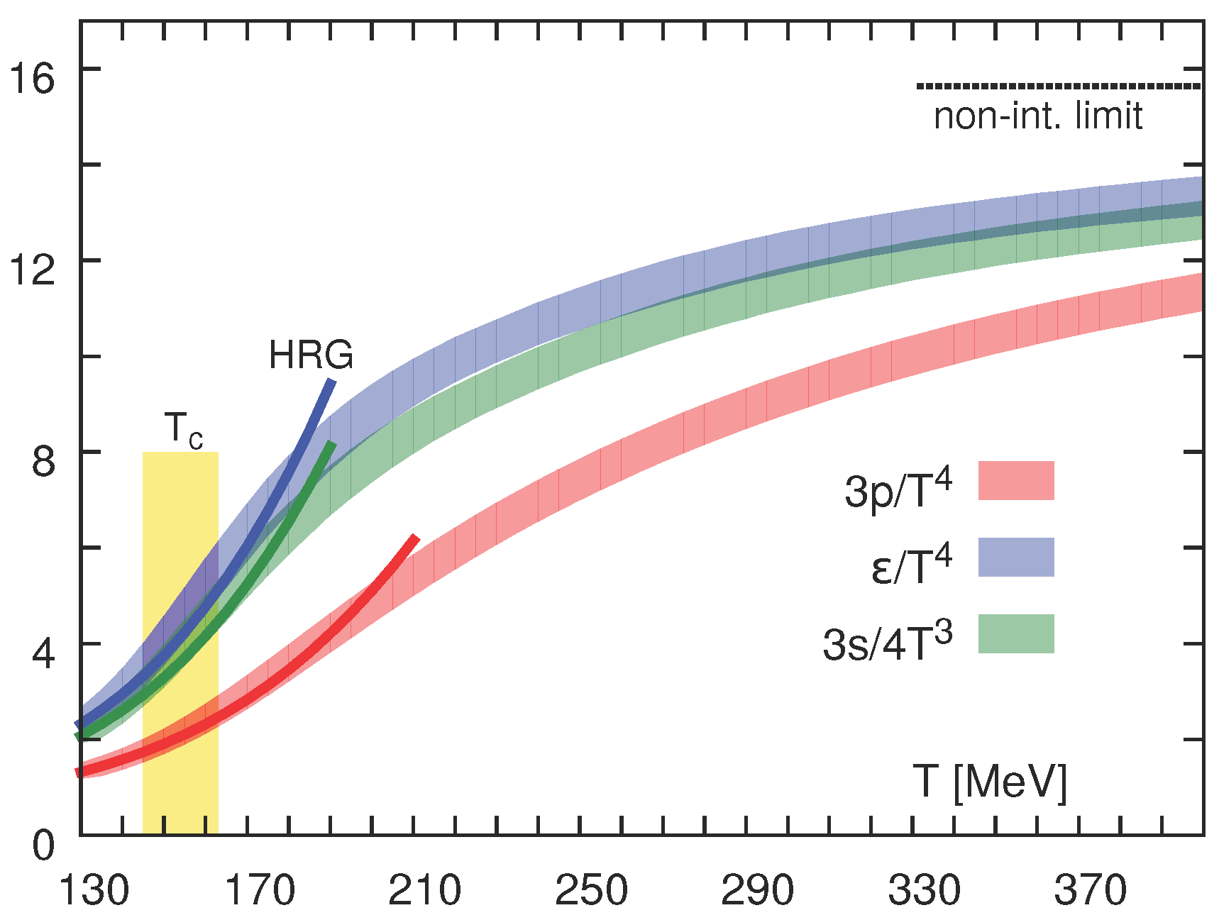
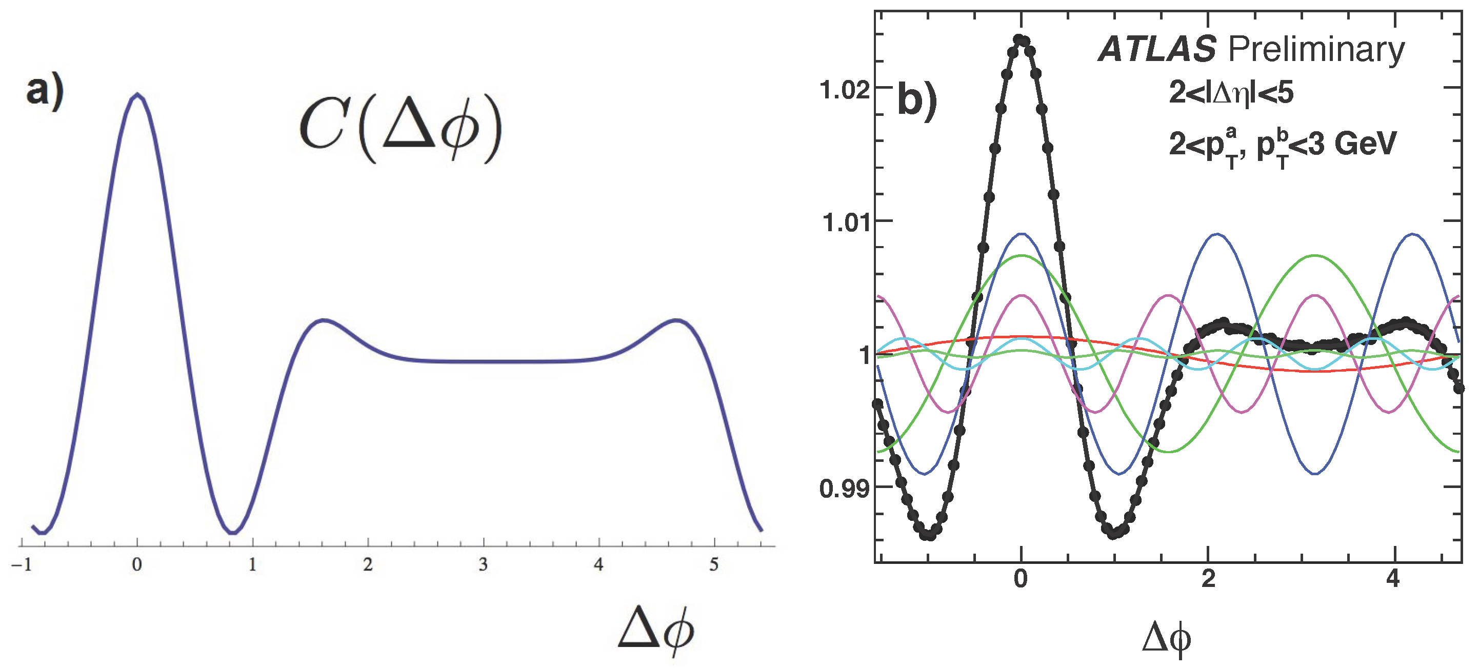
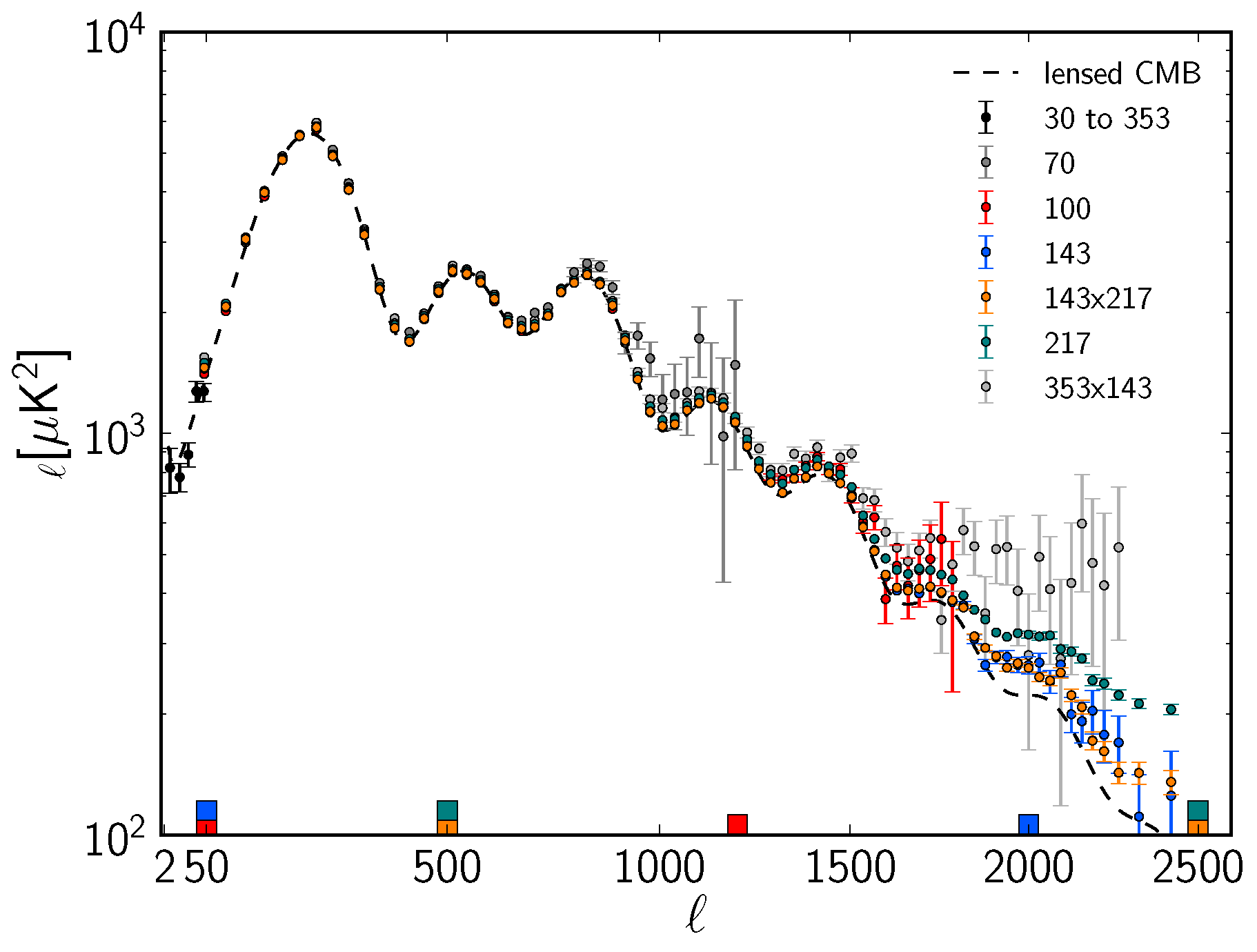
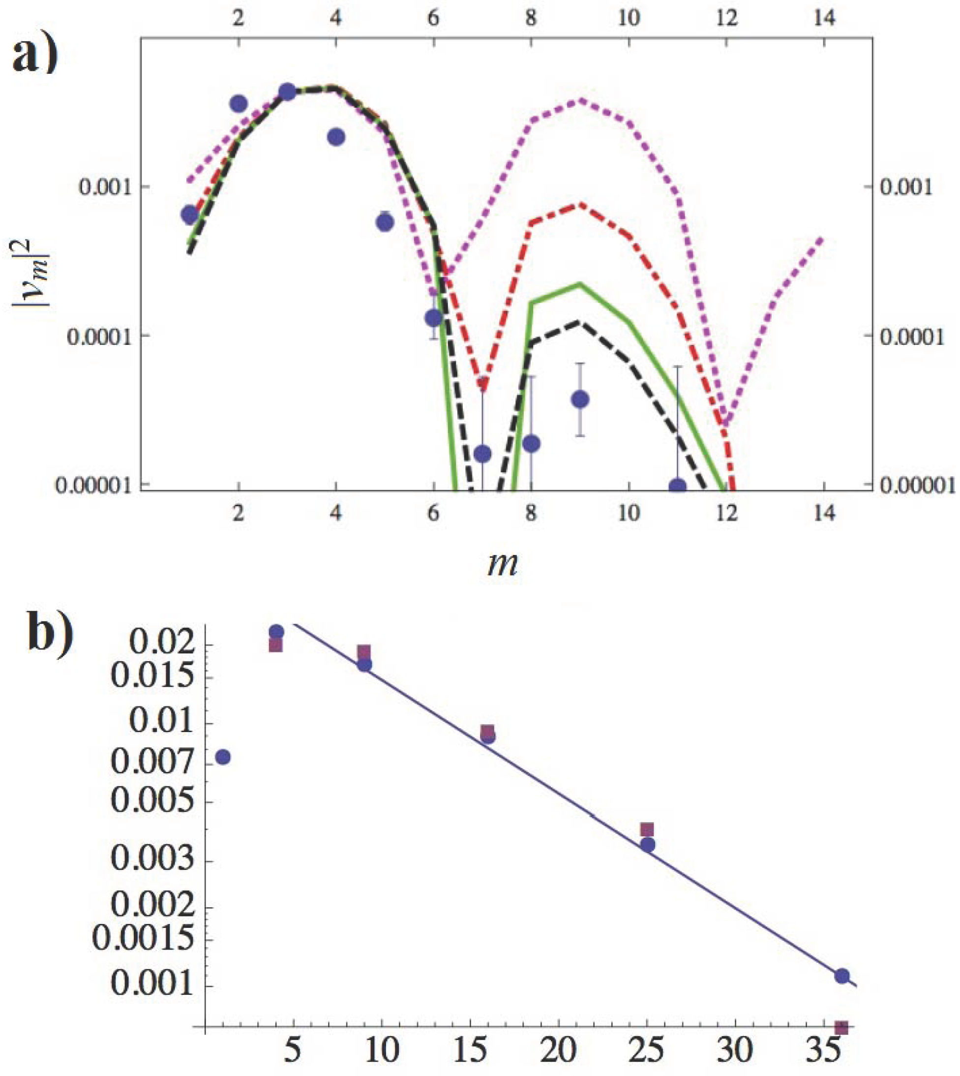
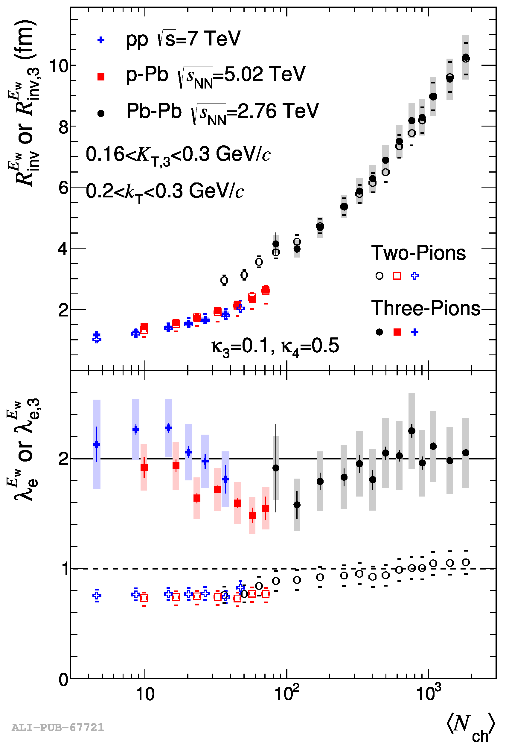
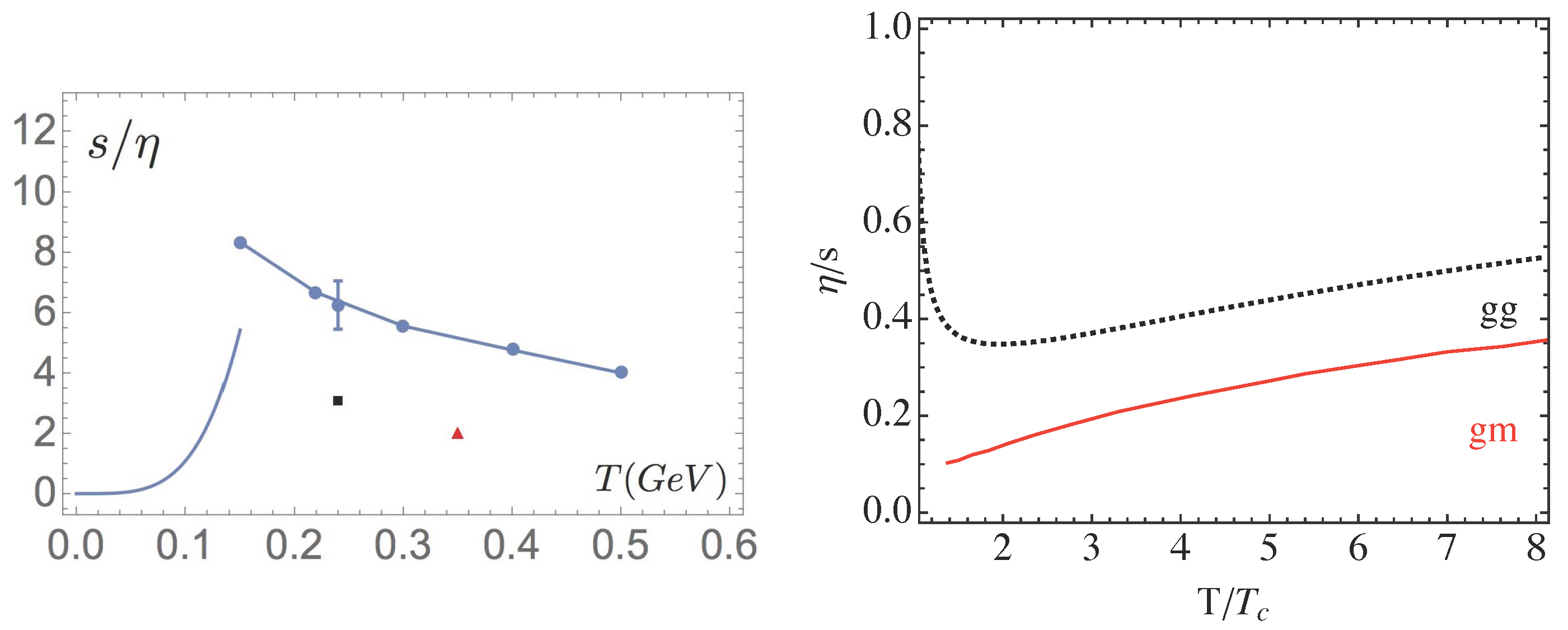
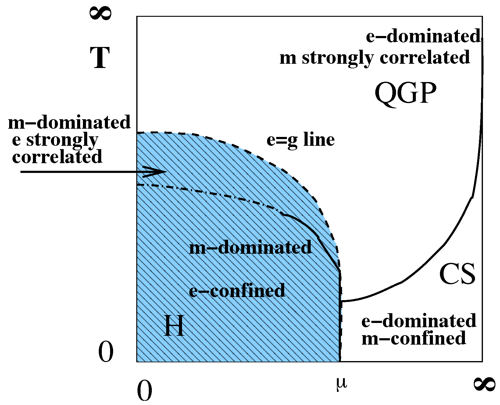
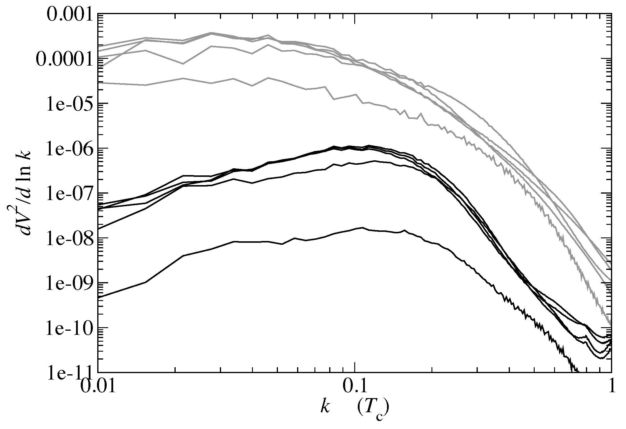
Table 1.
The electric and magnetic screening masses, normalized to the temperature. The last column is the square of their ratio.
© 2017 by the author. Licensee MDPI, Basel, Switzerland. This article is an open access article distributed under the terms and conditions of the Creative Commons Attribution (CC BY) license (http://creativecommons.org/licenses/by/4.0/).
Share and Cite
MDPI and ACS Style
Shuryak, E. The Sounds of the Little and Big Bangs. Universe 2017, 3, 75. https://doi.org/10.3390/universe3040075
AMA Style
Shuryak E. The Sounds of the Little and Big Bangs. Universe. 2017; 3(4):75. https://doi.org/10.3390/universe3040075
Chicago/Turabian StyleShuryak, Edward. 2017. "The Sounds of the Little and Big Bangs" Universe 3, no. 4: 75. https://doi.org/10.3390/universe3040075
APA StyleShuryak, E. (2017). The Sounds of the Little and Big Bangs. Universe, 3(4), 75. https://doi.org/10.3390/universe3040075
Note that from the first issue of 2016, this journal uses article numbers instead of page numbers. See further details here.