Testing General Relativity with the Radio Science Experiment of the BepiColombo mission to Mercury

Abstract

The relativity experiment is part of the Mercury Orbiter Radio science Experiment (MORE) on-board the ESA/JAXA BepiColombo mission to Mercury. Thanks to very precise radio tracking from the Earth and accelerometer, it will be possible to perform an accurate test of General Relativity, by constraining a number of post-Newtonian and related parameters with an unprecedented level of accuracy. The Celestial Mechanics Group of the University of Pisa developed a new dedicated software, ORBIT14, to perform the simulations and to determine simultaneously all the parameters of interest within a global least squares fit. After highlighting some critical issues, we report on the results of a full set of simulations, carried out in the most up-to-date mission scenario. For each parameter we discuss the achievable accuracy, in terms of a formal analysis through the covariance matrix and, furthermore, by the introduction of an alternative, more representative, estimation of the errors. We show that, for example, an accuracy of some parts in ${10}^{-6}$ for the Eddington parameter β and of ${10}^{-5}$ for the Nordtvedt parameter η can be attained, while accuracies at the level of $5\times {10}^{-7}$ and $1\times {10}^{-7}$ can be achieved for the preferred frames parameters ${\alpha }_1$ and ${\alpha }_2$, respectively.

1. Introduction

BepiColombo is a mission for the exploration of the planet Mercury, jointly developed by the European Space Agency (ESA) and the Japan Aerospace eXploration Agency (JAXA). The mission is scheduled for launch in April 2018 and for orbit insertion around Mercury at the end of 2024. The science mission consists of two separated spacecraft, which will be inserted in two different orbits around the planet: the Mercury Planetary Orbiter (MPO), devoted to the study of the surface and internal composition [1], and the Mercury Magnetospheric Orbiter (MMO), designed for the study of the planet’s magnetosphere [2]. In particular, the Mercury Orbiter Radio science Experiment (MORE) is one of the experiments on-board the MPO spacecraft.

Thanks to the state-of-the-art on-board and on-ground instrumentation [3], MORE will enable a better understanding of both Mercury geophysics and fundamental physics. The main goals of the MORE radio science experiment are concerned with the gravity of Mercury [4,5,6,7,8], the rotation of Mercury [9,10,11] and General Relativity (GR) tests [12,13,14,15,16]. The global experiment consists in determining the value and the formal uncertainty (as defined in Section 2.2) of a number of parameters of general interest, with the addition of further parameters characterizing each specific goal of the experiment. The quantities to be determined can be partitioned as follows:

(a)

spacecraft state vector (position and velocity) at given times (Mercurycentric orbit determination);

(b)

spherical harmonics of the gravity field of Mercury [17] and tidal Love number $k_2$ [18], in order to constrain physical models of the interior of Mercury (gravimetry experiment);

(c)

parameters defining the model of the Mercury’s rotation (rotation experiment);

(d)

digital calibrations for the Italian Spring Accelerometer (ISA) [19,20];

(e)

state vector of Mercury and Earth-Moon Barycenter (EMB) orbits at some reference epoch, in order to improve the ephemerides (Mercury and EMB orbit determination);

(f)

post-Newtonian (PN) parameters [12,13,21,22], together with some related parameters, like the solar oblateness factor $J_{2\odot }$, the solar gravitational factor ${\mu }_{\odot }=G{M}_{\odot }$, where G is the gravitational constant and $M_{\odot }$ the Sun’s mass, and its time variation, $\zeta =(1/{\mu }_{\odot })d{\mu }_{\odot }/dt$, in order to test gravitational theories (relativity experiment).

A good initial guess for each of the above parameters will also be necessary: for example, for the PN parameters we use the GR values, while for gravimetry we refer to the most recent MESSENGER results as nominal values in simulations [23].

To cope with the extreme complexity of MORE and its challenging goals, the Celestial Mechanics Group of the University of Pisa developed (under an Italian Space Agency commission) a dedicated software, ORBIT14, which is now ready for use. The software enables the generation of the simulated observables and the determination of the solve-for parameters by means of a global least squares fit.

In this paper, the results of a full set of simulations are discussed, carried out in the most up-to-date mission scenario [24], focusing on the parameters of interest for the relativity experiment. The paper is organized as follows: in Section 2 we describe in details the structure of the ORBIT14 software, while in Section 3 we introduce the mathematical models adopted to perform a full relativistic and coherent analysis of the observations. The simulation scenario and the adopted assumptions are detailed in Section 4, while the results are presented in Section 5, together with a comprehensive discussion on the achievable accuracies. Finally, conclusions are drawn in Section 6.

2. The ORBIT14 Software

The ORBIT14 software system has been developed by the Celestial Mechanics Group of the University of Pisa starting since 2007 as a new dedicated software for the MORE experiment. In Section 2.1 we describe the global structure of the software, while in Section 2.2 we briefly recall the non-linear least squares method. Details on the adopted multi-arc strategy are given in Section 2.3.

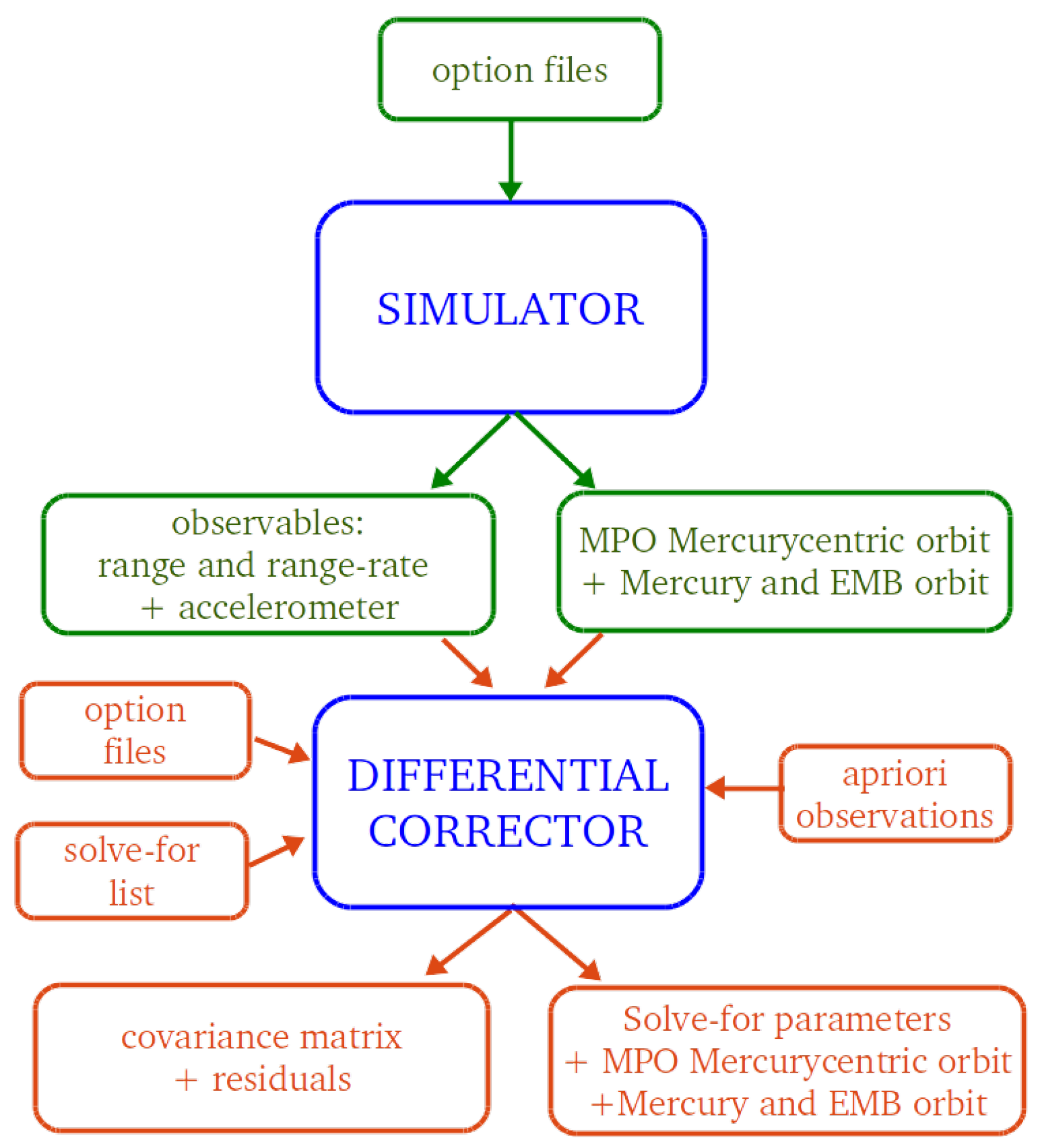
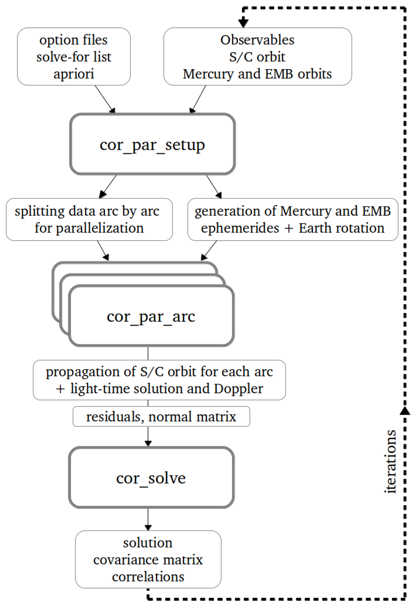
2.1. Global Structure

The global structure of the code is outlined in Figure 1. The main programs belong to two categories: data simulator (short: simulator) and differential corrector (short: corrector). Code is written in Fortran90 language. The simulator is needed to predict possible scientific results of the experiment. It generates simulated observables (range and range-rate, accelerometer readings) and the nominal value for orbital elements of the Mercurycentric orbit of the spacecraft, of Mercury and of the EMB orbits. The program structure of the simulator is quite simple if compared with the differential corrector, the most demanding part being the implementation of the dynamical, observational and error models.

The actual core of the code is the corrector, which solves for all the parameters $\mathbf{u}$ which can be determined by a least squares fit (possibly constrained and/or decomposed in a multi-arc structure). The corrector structure has been designed in order to exploit parallel computing, especially for the most computationally expensive portion of the processing. An outline of the steps involved in a single corrector’s iteration is shown in Figure 2.

2.2. Non-Linear Least Squares Fit

Following a classical approach (see, for instance, [25]—Chapter 5), the non-linear least squares (LS) fit leads to compute a set of parameters $\mathbf{u}$ which minimizes the following target function:

$$Q(\mathbf{u})=\frac{1}{m}{\mathbf{\xi }}^T(\mathbf{u})W\mathbf{\xi }(\mathbf{u})=\frac{1}{m}\sum _{i=1}^m{w}_i{\xi }_i^2(\mathbf{u}),$$

(1)

where m is the number of observations and $\mathbf{\xi }(\mathbf{u})=\mathcal{O}-\mathcal{C}(\mathbf{u})$ is the vector of residuals, i.e., the difference between the observed $\mathcal{O}$ and the predicted quantities $\mathcal{C}(\mathbf{u})$, computed following suitable mathematical models and assumptions. In our case, $\mathcal{O}$ are tracking data (range, range-rate and non-gravitational accelerations from the accelerometer), while $\mathcal{C}(\mathbf{u})$ are the results of the light-time computation (see [22] for details) as a function of all the parameters $\mathbf{u}$. Finally, $w_i$ is the weight associated to the i-th observation. Among the parameters $\mathbf{u}$, the ones introduced in Section 1 in (a), (b), (c) and (d) occur in the equation of motion of the Mercurycentric orbit of the spacecraft, while those in e) and f) occur in the equations of the orbits of Mercury and the Earth-Moon barycenter with respect to the Solar System Barycenter (SSB). Other information required for such orbit propagations are supposed to be known: positions and velocities of the other planets of the Solar System are obtained from the JPL ephemerides DE421 [26], while the rotation of the Earth is provided by the interpolation table made public by the International Earth Rotation Service (IERS: http://www.iers.org.) and the coordinates associated with the ground stations are expected to be available.

The procedure to compute ${\mathbf{u}}^{*}$, the set of parameters which minimizes $Q(\mathbf{u})$, is based on a modified Newton’s method known in the literature as differential corrections method. All the details can be found in [25]—Chapter 5. Let us define:

$$B=\frac{\partial \mathbf{\xi }}{\partial \mathbf{u}}(\mathbf{u}),C=B^{T}WB,$$

which are called design matrix and normal matrix, respectively. Then, the correction

$$\Delta \mathbf{u}=C^{-1}D\mathrm{with}D=-B^{T}W\mathbf{\xi }$$

is applied iteratively until either Q does not change meaningfully from one iteration to the other or $\Delta \mathbf{u}$ becomes smaller than a given tolerance. Introducing the inverse of the normal matrix, $\mathrm{\Gamma }=C^{-1}$, we always adopt the probabilistic interpretation of Γ as the covariance matrix of the vector $\mathbf{u}$, considered as a multivariate Gaussian distribution with mean ${\mathbf{u}}^{*}$ in the space of parameters.

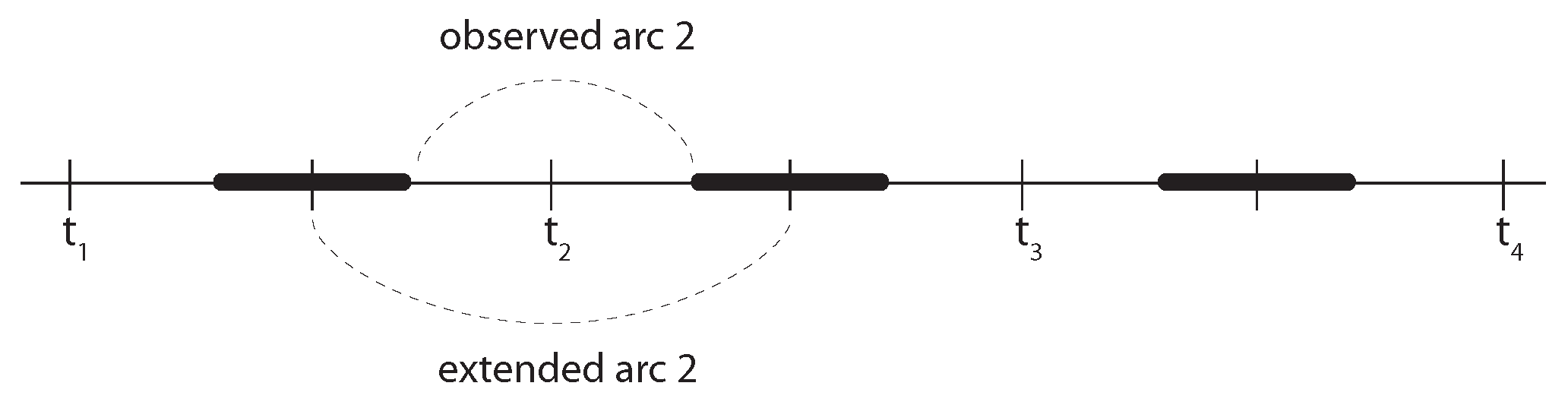
2.3. Pure and Constrained Multi-Arc Strategy

The tracking measurements from the Earth to the spacecraft are not continuous because of the mutual geometric configuration between the observing station and the antenna on the probe. The following visibility conditions are defined to account for: (i) the occultation of the spacecraft behind Mercury as seen from the Earth; (ii) the elevation of Mercury above the horizon at the observing station (the data received when Mercury is below a minimum elevation of 15${}^{\circ }$ from the horizon are discarded because they are too noisy and could degrade the results); (iii) the angle between Mercury and the Sun as seen from the Earth. As a result, the observations are split in arcs, with a duration of ∼24 h. Considering two observing stations (see Section 4), the adopted visibility conditions provide tracking sessions with an average duration of 15–16 h, called observed arcs, followed by a period of some hours without observations.

In orbit determination, the estimation approach consists of a combined solution called multi-arc strategy (see, e.g., [25]). According to this method, every single arc of observations has its own set of initial conditions (position and velocity at the reference central epoch of the considered time interval), as it belongs to a different object. In this way, due to lack of knowledge in the dynamical models, the actual errors in the orbit propagation can be reduced by an over-parameterization of the initial conditions. A different choice has been made in ORBIT14, implementing the so called constrained multi-arc strategy [10,14,27]. The method is based on the idea that each observed arc belongs to the same object (the spacecraft). First of all, an extended arc is defined as the observed arc broadened to half the preceding and to half the following periods without tracking, as shown in Figure 3. The orbits of two consecutive extended arcs should coincide at the connection time in the middle of the non-observed interval. We refer to [10,27] for a complete description of the constrained multi-arc strategy.

In the constrained multi-arc approach, the parameters $\mathbf{u}$ can be classified, depending on the arc they refer to, as:

• Global Parameters ($\mathbf{g}$): parameters that affect the dynamical equations of every observed (and extended) arc. The PN parameters and the spherical harmonic coefficients of Mercury are an example.
• Local Parameters (${\mathbf{l}}^k$): parameters that affect the dynamical equations of a single observed arc k. The state vector of the Mercurycentric orbit associated with the arc and the desaturation manoeuvres applied during the tracking are few examples.
• Local External Parameters (${\mathbf{le}}^{k,k+1}$): parameters that affect only the dynamical equations in the period without tracking between two subsequent observed arcs k and $k+1$. These are the desaturation maneuvres taking place out of the observed arcs.

To implement the constrained multi-arc strategy in the framework of the LS fit described in Section 2.2, we define the discrepancy vector between the k and $k+1$ arcs, ${\mathbf{d}}^{k,k+1}$, as:

$${\mathbf{d}}^{k,k+1}=\Phi (t_c^k;t_0^{k+1},{\mathbf{X}}_0^{k+1})-\Phi (t_c^k;t_0^k,{\mathbf{X}}_0^k),$$

where $t_0^k$ and $t_0^{k+1}$ denote the central time of the k and $k+1$ arc, respectively, $t_c^k$ is the connection time between the two extended k and $k+1$ arcs, ${\mathbf{X}}_0^k$ and ${\mathbf{X}}_0^{k+1}$ are the state vector at $t_0^k$ and $t_0^{k+1}$, respectively, and $\Phi (t_c^k;t_0^{k+1},{\mathbf{X}}_0^{k+1})$ is the image of $(t_0^{k+1},{\mathbf{X}}_0^{k+1})$ under the flow of the vector field associated with the Mercurycentric orbit at time $t=t_c^k$ (analogously for $\Phi (t_c^k;t_0^k,{\mathbf{X}}_0^k)$). Thus, we have:

$${\mathbf{d}}^{k,k+1}={\mathbf{d}}^{k,k+1}(g,l^k,l{e}^{k,k+1},l^{k+1}),$$

where g, $l^k$, $l{e}^{k,k+1}$ are the parameters $\mathbf{u}$ included in the LS fit, classified, respectively, as global (g), local ($l^k$) for the k-th arc and local external ($l{e}^{k,k+1}$) between the k-th and $(k+1)$-th arcs. The constrained multi-arc strategy consists in minimizing the target function:

$$\begin{array}{cc}\hfill Q(\mathbf{u})& =\frac{1}{m+6(n-1)}\sum _{i=1}^m{w}_i{\xi }_i^2+\hfill \\ & +\frac{1}{\mu }\frac{1}{m+6(n-1)}\sum _{k=1}^{n-1}{\mathbf{d}}^{k,k+1}·C^{k,k+1}{\mathbf{d}}^{k,k+1},\hfill \end{array}$$

where n is the total number of extended arcs, μ is a penalty parameter and $C^{k,k+1}$ is a weight matrix for the discrepancy vectors. Two possible approaches can be followed. The first is called internally constrained multi-arc strategy. In this case, we consider the confidence ellipsoids associated with ${\mathbf{X}}_0^k$ and ${\mathbf{X}}_0^{k+1}$ at $t_0^k$ and $t_0^{k+1}$, respectively, and we propagate them to $t_c^k$ through the corresponding state transition matrices. This means that we expect ${\mathbf{d}}^{k,k+1}$ to be normally distributed with mean $\Phi (t_c^k;t_0^{k+1},{\mathbf{X}}_0^{k+1})-\Phi (t_c^k;t_0^k,{\mathbf{X}}_0^k)$ and covariance

$${\mathrm{\Gamma }}_c:={(C^k)}^{-1}+{(C^{k+1})}^{-1},$$

where $C^k$ and $C^{k+1}$ are the $6\times 6$ normal matrices associated with ${\mathbf{X}}_0^k$ and ${\mathbf{X}}_0^{k+1}$ at $t_0^k$ and $t_0^{k+1}$ and propagated to $t_c^k$, respectively. It follows that

$$C^{k,k+1}={\mathrm{\Gamma }}_c^{-1}\mathrm{and}\mu =1.$$

The second approach is called apriori constrained multi-arc strategy and it takes care of the degeneracy in orbit determination due to the orbit geometry (details can be found in [28]). In particular, we deal with an approximated version of the exact symmetry described in [28], where the small parameter of the perturbation is the angle of displacement of the Earth-Mercury vector in an inertial frame. In this case, the normal matrix has one eigenvalue significantly smaller than the others. As a consequence of this weakness, the confidence ellipsoid associated with the discrepancy and defined by $C^{k,k+1}$ could be very elongated. The basic idea of this approach is to constrain the discrepancy ${\mathbf{d}}^{k,k+1}$ inside a sphere of given radius, that can be suitably shrunk by varying μ. This can be interpreted as adding apriori observations. On the contrary, in the internally constrained multi-arc strategy, the discrepancy is constrained inside the intersection of the two ellipsoids propagated from $t_0^k$ and $t_0^{k+1}$. All the details are extensively explained in [27]. For the results presented in this review, we will always adopt an apriori constrained multi-arc strategy. Finally, it can be noted that in the multi-arc method the residuals ξ depend only on global and local parameters, and this applies to the target function Q defined in Equation (1) as well.

3. Mathematical Models

The purpose of the MORE relativity experiment is to perform a test of General Relativity comparing theory with experiment. The majority of the Solar System tests of gravitation can be set in the context of the slow-motion, weak field limit [29], usually known as the post-Newtonian approximation. In this limit, the space-time metric can be written as an expansion about the Minkowski metric in terms of dimensionless gravitational potentials. In the parametrized PN formalism, each potential term in the metric is expressed by a specific parameter, which measures a general property of the metric. The basic idea of the MORE relativity experiment is to investigate the dependence of the equation of motion from the PN parameters. By isolating the effects of each parameter on the motion, it is possible to constrain the parameters values within some accuracy threshold, testing the validity of GR predictions.

The PN parameters of interest for our analysis are the following:

• the Eddington parameters β and γ. β accounts for the modification of the non-linear three-body general relativistic interaction and γ parametrizes the velocity-dependent modification of the two-body interaction and accounts also for the space-time curvature through the Shapiro effect [30]. These are the only non-zero PN parameters in GR (they are both equal to unity);
• the Nordtvedt parameter η. The effect of η in the equations of motion is to produce a polarization of the Mercury and Earth orbits in the gravitational field of the other planets and it is related to possible violations of the Strong Equivalence Principle (see, e.g., the discussion in [31]);
• the preferred frame effects parameters ${\alpha }_1$ and ${\alpha }_2$. They phenomenologically describe the effects due to the presence of a gravitationally preferred frame; we follow the standard assumption to identify the preferred frame with the rest frame of the cosmic microwave background [32].

Beside the five PN parameters mentioned above, we consider a few additional parameters. These do not properly produce relativistic effects, but the uncertainty in their knowledge generates orbital effects at least comparable with the perturbations expected from the tested relativistic parameters. We consider two kinds of “Newtonian” orbital effects: a small change in the Sun’s gravity oblateness $J_{2\odot }$ and a small change in the Sun’s gravitational factor ${\mu }_{\odot }=G{M}_{\odot }$, where G is the gravitational constant and $M_{\odot }$ is the Sun’s mass. Regarding the second quantity, since many alternative theories of gravitation allow for a possible time variation of the gravitational constant, we included in the solve-for parameters the time derivative of ${\mu }_{\odot }$ described by the parameter $\zeta =\frac{1}{{\mu }_{\odot }}\frac{d{\mu }_{\odot }}{dt}$. Indeed, within the MORE experiment we cannot discriminate between a time variation of $M_{\odot }$ or G, but assuming an independent estimate for the rate of $M_{\odot }$, it could be possible to draw information on the time rate of G.

The effects linked to each PN parameter, corresponding to modifications of the space-time metric, affect both the propagation of the tracking signal (range and range-rate) and the equations of motion. In the following we describe the mathematical models adopted in our analysis: in Section 3.1 we define the computed tracking observables in a coherent relativistic background and in Section 3.2 we present the Langrangian formulation of the planetary dynamics in the context of the first-order PN approximation. Finally, in Section 3.3 we define the Mercurycentric dynamical model.

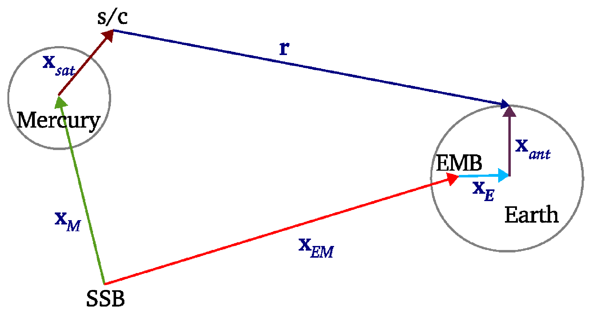
3.1. Computation of Observables

In a radio science experiment, the observational technique is complicated by many factors (for example plasma reduction) but in simulations it can be merely considered as a tracking from an Earth-based station, giving range and range-rate information (see, e.g., [3]). In order to compute the range distance from the ground station on the Earth to the spacecraft around Mercury (or in an interplanetary trajectory), and the corresponding range-rate, we introduce the following state vectors, each one evolving according to a specific dynamical model (see Figure 4):

• the Mercurycentric position of the spacecraft, ${\mathbf{x}}_{sat}$;
• the SSB positions of Mercury and of the EMB, ${\mathbf{x}}_M$ and ${\mathbf{x}}_{EM}$;
• the geocentric position of the ground antenna, ${\mathbf{x}}_{ant}$;
• the position of the Earth barycenter with respect to the EMB, ${\mathbf{x}}_E$.

They can be combined to define the range distance using the following formula, as a first approximation:

$$r=\left|\mathbf{r}\right|=|({\mathbf{x}}_{sat}+{\mathbf{x}}_M)-({\mathbf{x}}_{EM}+{\mathbf{x}}_E+{\mathbf{x}}_{ant})|.$$

(2)

As explained in [22], Equation (2) corresponds to model the space as a flat arena (r is the Euclidean distance) and the time as an absolute parameter. Obviously, this is not a suitable assumption, since it is clear that beyond some threshold of accuracy, as expected for the BepiColombo radio science experiment, space and time must be formulated in the framework of General Relativity. Moreover, we have to take into account the different times at which the events have to be computed: the transmission of the signal at the transmitting time ($t_t$), the signal at the Mercury orbiter at the time of bounce ($t_b$) and the reception of the signal at the receiving time ($t_r$). Equation (2) can be used as a starting point to construct a correct relativistic formulation, containing not all the possible relativistic effects, but the ones which are measurable in the experiment.

The five vectors in Equation (2) have to be computed at their own time, which corresponds to the epoch of different events: e.g., ${\mathbf{x}}_{ant}$, ${\mathbf{x}}_{EM}$ and ${\mathbf{x}}_E$ are computed at both the antenna transmission time $t_t$ and receiving time $t_r$ of the signal, while ${\mathbf{x}}_M$ and ${\mathbf{x}}_{sat}$ are computed at the bounce time $t_b$ (when the signal has reached the orbiter and is sent back, with correction for the delay of the transponder). To perform the vectorial sums and differences, these vectors must be converted to a common space-time reference system, the only possible choice being some realization of the BCRS (Barycentric Celestial Reference System). We adopt a realization of the BCRS that we call SSB (Solar System Barycentric) reference frame in which the time is a re-definition of the TDB (Barycentric Dynamic Time), according to the IAU 2006 Resolution B3 (https://www.iau.org/static/resolutions/IAU2006_Resol3.pdf). Other possible choices, such as TCB (Barycentric Coordinate Time), can only differ by linear scaling. The TDB choice of the SSB time scale entails also the appropriate linear scaling of space-coordinates and planetary masses as described, for instance, in [33,34].

The vectors ${\mathbf{x}}_M$, ${\mathbf{x}}_E$, and ${\mathbf{x}}_{EM}$ are already in the SSB reference frame as provided by numerical integration and external ephemerides, while the vectors ${\mathbf{x}}_{ant}$ and ${\mathbf{x}}_{sat}$ must be converted to SSB from the geocentric and Mercurycentric systems, respectively. Of course, the conversion of reference systems implies also the conversion of the time coordinate. There are three different time coordinates to be considered. The currently published planetary ephemerides are provided in TDB. The observations from the Earth are based on averages of clock and frequency measurements on the Earth surface: this defines another time coordinate called TT (Terrestrial Time). Thus for each observation the times of transmission $t_t$ and reception $t_r$ need to be converted from TT to TDB to find the corresponding positions of the planets. This time conversion step is necessary for the accurate processing of each set of interplanetary tracking data. The main term in the difference TT-TDB is periodic, with period 1 year and amplitude ≃1.6 $\times {10}^{-3}$ s, while there is essentially no linear trend, as a result of a suitable definition of the TDB. Finally, the equation of motion of the spacecraft orbiting Mercury has been approximated, to the required level of accuracy, following what done in [35] for the case of a near-Earth spacecraft in a geocentric frame of reference. We consider the Newtonian dynamics in a local Mercurycentric frame assuming as independent variable a suitably defined time coordinate. Moreover, we add the relativistic perturbative acceleration from the one-body Schwarzschild isotropic metric for Mercury and the acceleration due to the geodesic precession, as explained in [10]. Thus, for MORE we have defined a new time coordinate TDM (Mercury Dynamic Time), as described in [13], containing terms of 1-PN order depending mostly upon the distance from the Sun and velocity of Mercury.

In general, the differential equation giving the local time T (in our case TT or TDM) as a function of the SSB time t, which we are currently assuming to be TDB, is the following:

$$\frac{dT}{dt}=1-\frac{1}{c^2}\left[U+\frac{v^2}{2}-L\right],$$

(3)

where U is the gravitational potential (the list of contributing bodies depends upon the required accuracy: in our implementation we use Sun, Mercury to Neptune, Moon) at the planet center and v is the velocity with respect to the SSB of the same planet. The constant term L is used to perform the conventional rescaling motivated by removal of secular terms [36].

The space-time transformations needed to coherently compute the vector ${\mathbf{x}}_{ant}$ involve essentially the position of the antenna and of the orbiter. The geocentric coordinates of the antenna should be transformed into TDB-compatible coordinates [34]. The transformation is expressed by:

$${\mathbf{x}}_{ant}^{TDB}={\mathbf{x}}_{ant}^{TT}\left(1-\frac{U}{c^2}-L_C\right)-\frac{1}{2}\left(\frac{{\mathbf{v}}_E^{TDB}·{\mathbf{x}}_{ant}^{TT}}{c^2}\right){\mathbf{v}}_E^{TDB},$$

where U is the gravitational potential at the geocenter (excluding the Earth mass), $L_C=1.48082686741\times {10}^{-8}$ is a scaling factor given as definition [37], supposed to be a good approximation for removing secular terms from the transformation and ${\mathbf{v}}_E^{TDB}$ is the barycentric velocity of the Earth. The following equation contains the effect on the velocities of the time coordinate change, which should be consistently used together with the coordinate change:

$${\mathbf{v}}_{ant}^{TDB}=\left[{\mathbf{v}}_{ant}^{TT}\left(1-\frac{U}{c^2}-L_C\right)-\frac{1}{2}\left(\frac{{\mathbf{v}}_E^{TDB}·{\mathbf{v}}_{ant}^{TT}}{c^2}\right){\mathbf{v}}_E^{TDB}\right]\left[\frac{dT}{dt}\right].$$

Note that the previous formula contains the factor $dT/dt$ (expressed by Equation (3)) that deals with a time transformation: T is the local time for Earth, that is TT, and t is the corresponding TDB time. To compute the coordinates of the orbiter (vector ${\mathbf{x}}_{sat}$) we adopt similar equations, as discussed in [22], where we neglected the terms of the SSB acceleration of the planet center [38], because they contain, beside $1/c^2$, the additional small parameter distance from planet center divided by planet distance to the Sun, which is of the order of ${10}^{-4}$ even for a Mercury orbiter.

In Figure 5 the behaviour of the range and range-rate observable, computed with and without the just explained relativistic corrections, is shown. It is quite evident that the differences are significant, at a signal-to-noise ratio $S/N\simeq 1$ for range, much larger for range-rate, with an especially strong signature from the orbital velocity of the Mercurycentric orbit (with $S/N>50$).

3.2. Dynamical Relativistic Models

To constrain the PN and related parameters, we need to determine the orbit of Mercury. A relativistic model for the motion of the planet is necessary. We choose to start from a Lagrangian formulation (see, e.g., [21]) in order to compute the terms of accelerations to be included in the right-hand side of the differential equations for Mercury and EMB (the dynamics of the other planets, as well as the relative EMB-Earth position, are given by the JPL ephemerides). In particular, let us assume that the motion of the considered planets is described by the sum of different Lagrangians:

$$L=L_{New}+L_{GR}+(\gamma -1)L_{\gamma }+(\beta -1)L_{\beta }+\zeta L_{\zeta }+J_{2\odot }{L}_{J2\odot }+{\alpha }_1{L}_{{\alpha }_1}+{\alpha }_2{L}_{{\alpha }_2}+\eta L_{\eta },$$

(4)

where $L_{New}$ is the Lagrangian of the Newtonian N-body problem, $L_{GR}$ is the corrective term taking into account General Relativity in the post-Newtonian approximation, $L_{\gamma }$ and $L_{\beta }$ are the terms taking into account the PN parameters γ and β, respectively, $L_{\zeta }$ is the Lagrangian for the time variation of the gravitational parameter of the Sun ${\mu }_{\odot }=G{M}_{\odot }$, $L_{J2\odot }$ takes into account the effect of the oblateness of the Sun, $L_{{\alpha }_1}$, $L_{{\alpha }_2}$ describe the preferred-frame effects through the parameters ${\alpha }_1$, ${\alpha }_2$, and, finally, $L_{\eta }$ checks for possible violations of the strong equivalence principle (see [12,13,31]).

To express the Lagrangian terms, we follow the notation of [35] and we introduce two parameters: the total mass of EMB, ${\mu }_{EMB}$, which is the sum of the gravitational parameter of the Earth and the Moon, and the mass ratio, $\overline{\mu }$, defined as the ratio of the gravitational parameter of the Earth over that of the Moon; both quantities ${\mu }_{EMB}$ and $\overline{\mu }$ are assumed to be fixed, hence we do not solve for them. Defining ${\mu }_E=\overline{\mu }/(1+\overline{\mu })$ and ${\mu }_{Moon}=1/(1+\overline{\mu })$, we have:

$${\mathbf{r}}_{EM}={\mu }_E{\mathbf{r}}_{Earth}+{\mu }_{Moon}{\mathbf{r}}_{Moon}$$

with analogous expressions for velocity and acceleration.

Notice that the usual Lagrangians are multiplied by G, so that only ${\mu }_i=G{M}_i$ appear in the overall Lagrangian. Indeed, the gravitational constant cannot be determined from any form of orbit determination (apart artificial systems). In the following we give the explicit expressions for each Lagrangian term in Equation (4).

• N-body Newtonian Lagrangian:

  $$L_{New}=\frac{1}{2}\sum _i{\mu }_i{v}_i^2+\frac{1}{2}\sum _i\sum _{j\ne i}\frac{{\mu }_i{\mu }_j}{r_{ij}}.$$
• Post-Newtonian General Relativistic Lagrangian:

  $$\begin{array}{ccc}\hfill L_{GR}& =& \frac{1}{8c^2}\sum _i{\mu }_i{v}_i^4-\frac{1}{2c^2}\sum _i\sum _{j\ne i}\sum _{k\ne i}\frac{{\mu }_i{\mu }_j{\mu }_k}{r_{ij}{r}_{ik}}+\hfill \\ & +& \frac{1}{2}\sum _i\sum _{j\ne i}\frac{{\mu }_i{\mu }_j}{r_{ij}}\left[\frac{3}{2c^2}(v_i^2+v_j^2)-\frac{7}{2c^2}({\mathbf{v}}_{\mathbf{i}}·{\mathbf{v}}_{\mathbf{j}})-\frac{1}{2c^2}({\mathbf{n}}_{\mathbf{ij}}·{\mathbf{v}}_{\mathbf{i}})({\mathbf{n}}_{\mathbf{ij}}·{\mathbf{v}}_{\mathbf{j}})\right].\hfill \end{array}$$
• Lagrangian for PN parameter γ:

  $$L_{\gamma }=\frac{1}{2c^2}\sum _i\sum _{j\ne i}\frac{{\mu }_i{\mu }_j}{r_{ij}}{({\mathbf{v}}_{\mathbf{i}}-{\mathbf{v}}_{\mathbf{j}})}^2.$$
• Lagrangian for PN parameter β:

  $$L_{\beta }=-\frac{1}{c^2}\sum _i\sum _{j\ne i}\sum _{k\ne i}\frac{{\mu }_i{\mu }_j{\mu }_k}{r_{ij}{r}_{ik}}.$$
• Lagrangian for parameter ζ:
  $L_{\zeta }$ describes the effect of a time variation of the gravitational parameter of the Sun, ${\mu }_{\odot }$:

  $${\mu }_{\odot }={\mu }_{\odot }(t_0)+{\dot{\mu }}_{\odot }(t_0)(t-t_0)+\dots ;$$

  defining

  $$\zeta =\frac{{\dot{\mu }}_{\odot }(t_0)}{{\mu }_{\odot }(t_0)}=\frac{d}{dt}ln{\mu }_{\odot }(t_0),$$

  we have:

  $$L_{\zeta }=(t-t_0)\sum _{i\ne 0}\frac{{\mu }_{\odot }{\mu }_i}{r_{0i}}.$$
• Lagrangian for ${\mathbf{J}}_{\mathbf{2}\odot }$ effect:

  $$L_{J_{2\odot }}=-\frac{1}{2}\sum _{i\ne 0}\frac{{\mu }_0{\mu }_i}{r_{0i}}{\left(\frac{R_{\odot }}{r_{0i}}\right)}^2[3{({\mathbf{n}}_{0i}·{\mathbf{e}}_0)}^2-1],$$

  where $R_{\odot }$ is the radius of the Sun, ${\mathbf{n}}_{0i}={\mathbf{r}}_{0i}/r_{0i}$ is the heliocentric position of body i and ${\mathbf{e}}_0$ is the unit vector along the rotation axis of the Sun. The unit vector ${\mathbf{e}}_0$ is given in standard equatorial coordinates with equinox J2000 at epoch J2000.0 (JD 2451545.0 TCB): ${\alpha }_0={286.13}^{\circ }$, ${\delta }_0={63.87}^{\circ }$ [39].
• Lagrangian for preferred frame effects, PN ${\alpha }_1$ and ${\alpha }_2$:

  $$L_{{\alpha }_1}=-\frac{1}{4c^2}\sum _j\sum _{i\ne j}\frac{{\mu }_i{\mu }_j}{r_{ij}}\left({\mathbf{z}}_i·{\mathbf{z}}_j\right),$$

  $$L_{{\alpha }_2}=\frac{1}{4c^2}\sum _j\sum _{i\ne j}\frac{{\mu }_i{\mu }_j}{r_{ij}}\left[\left({\mathbf{z}}_i·{\mathbf{z}}_j\right)-\left({\mathbf{n}}_{\mathbf{i}\mathbf{j}}·{\mathbf{z}}_i\right)\left({\mathbf{n}}_{\mathbf{i}\mathbf{j}}·{\mathbf{z}}_j\right)\right],$$

  where ${\mathbf{z}}_i=\mathbf{w}+{\mathbf{v}}_{\mathbf{i}}$ and $\mathbf{w}$ is the velocity of the considered reference system with respect to the PN preferred reference frame, which is a reference frame whose outer regions are at rest with respect to the universe rest frame (see [21]). In the case of the SSB reference frame, that could be the one of cosmic microwave background, $\left|\mathbf{w}\right|=370\pm 10$ km/s, in the direction $(\alpha ,\delta )=({168}^{\circ },7^{\circ })$ in the Equatorial J2000 reference frame (see [12]). Notice that we can combine the two previous Lagrangians and the parameters ${\alpha }_1$ and ${\alpha }_2$ obtaining an unique Lagrangian for the preferred frame effects:

  $$\begin{array}{ccc}\hfill L_{\alpha }={\alpha }_1{L}_{{\alpha }_1}+{\alpha }_2{L}_{{\alpha }_2}& =& \frac{{\alpha }_2-{\alpha }_1}{4c^2}\sum _j\sum _{i\ne j}\frac{{\mu }_i{\mu }_j}{r_{ij}}({\mathbf{v}}_{\mathbf{i}}+\mathbf{w})·({\mathbf{v}}_{\mathbf{j}}+\mathbf{w})+\hfill \\ & -& \frac{{\alpha }_2}{4c^2}\sum _j\sum _{i\ne j}({\mathbf{r}}_{\mathbf{j}\mathbf{i}}·({\mathbf{v}}_{\mathbf{j}}+\mathbf{w}))({\mathbf{r}}_{\mathbf{j}\mathbf{i}}·({\mathbf{v}}_{\mathbf{i}}+\mathbf{w}))\frac{{\mu }_i{\mu }_j}{r_{ij}^3}.\hfill \end{array}$$
• Lagrangian for possible violation of the equivalence principle, PN η:
  With the Lagrangian multiplied by G, the Newtonian kinetic energy is:

  $$T=\frac{1}{2}\sum _i{\mu }_i{v}_i^2,$$

  where we assume that the inertial mass and the gravitational mass are the same (or, at least, exactly proportional). If some form of mass has a different gravitational coupling, there are, for each body i, two quantities ${\mu }_i$ and ${\mu }_i^I$, one appearing in the gravitational potential (including the relativistic part) and the other appearing in the kinetic energy. If there is a violation of the strong equivalence principle involving body i, with a fraction ${\Omega }_i$ of its mass due to gravitational self-energy (for the moment we are using the approximation of constant density: ${\Omega }_i=-3{\mu }_i/5R{c}^2$; notice that ${\Omega }_i$ is $O(c^{-2})$):

  $${\mu }_i=(1+\eta {\Omega }_i){\mu }_i^I⟺{\mu }_i^I=(1-\eta {\Omega }_i){\mu }_i+\mathcal{O}({\eta }^2)$$

  with η the PN parameter for this violation. Neglecting $\mathcal{O}({\eta }^2)$ terms (and also $\mathcal{O}[\eta (\gamma -1)],..$) this is expressed by a Lagrangian term $\eta L_{\eta }$, where:

  $$L_{\eta }=-\frac{1}{2}\sum _i{\Omega }_i{\mu }_i{v}_i^2.$$

Considering an inertial reference system, the equations of motion for the i-th body are described by the Lagrangian equations:

$$\frac{d}{dt}\frac{\partial L}{\partial {\mathbf{v}}_i}=\frac{\partial L}{\partial {\mathbf{r}}_i},$$

which in general give an implicit expression for the acceleration of the form $f({\mathbf{a}}_i)=g({\mathbf{r}}_i,{\mathbf{v}}_i)$. However, since the main term is the N-body Newtonian acceleration ${\mathbf{a}}_i^{New}$ and the other terms are small perturbations, we can use the following approximation for the total acceleration of the i-th body:

$${\mu }_i{\mathbf{a}}_i={\mu }_i{\mathbf{a}}_i^{New}+\frac{\partial (L-L_{New})}{\partial {\mathbf{r}}_i}-\left[\frac{d}{dt}\frac{\partial (L-L_{New})}{\partial {\mathbf{v}}_i}\right]\left|{}_{{\mathbf{a}}_i={\mathbf{a}}_i^{New}}\right..$$

If we call $Y={[{\mathbf{r}}_1,{\mathbf{r}}_{EM},{\mathbf{v}}_1,{\mathbf{v}}_{EM}]}^T$ the 12-dimensional state vector (for Mercury and EMB) we want to propagate, we can write the equations of motion in the more complete form:

$$\frac{d}{dt}Y=\left(\begin{array}{c}{\mathbf{v}}_1\\ {\mathbf{v}}_{EM}\\ {\mathbf{a}}_1\\ {\mathbf{a}}_{EM}\end{array}\right)=F({\mathbf{r}}_1,{\mathbf{r}}_{EM},{\mathbf{v}}_1,{\mathbf{v}}_{EM},...).$$

The reference system for these dynamics is centered in the SSB, and it is inertial in the PN approximation. On the other hand, if we consider possible violations, as it happens in the case of parameterized PN formalism, we need to reassess the total linear momentum conservation theorem. Using Noether’s theorem we can compute the integral of the total linear momentum of the system:

$$\frac{d}{dt}\mathbf{P}=0,where\mathbf{P}=\sum _i\frac{\partial L}{\partial {\mathbf{v}}_{\mathbf{i}}}.$$

Since $L_{\beta }$, $L_{\zeta }$, $L_{J2\odot }$ do not depend on velocities and, because of the antisimmetry, we have that ${\sum }_i\frac{\partial L_{\gamma }}{\partial {\mathbf{v}}_{\mathbf{i}}}=0$ and $L_{\gamma }$ does not contribute; thus, the total linear momentum of the system reads:

$$\mathbf{P}=\sum _i\frac{\partial (L_{New}+L_{GR}+L_{\alpha }+\eta L_{\eta })}{\partial {\mathbf{v}}_{\mathbf{i}}}.$$

In the PN approximation the total linear momentum is simply:

$$\begin{array}{ccc}\hfill \mathbf{P}& =& \sum _i\frac{\partial (L_{New}+L_{GR})}{\partial {\mathbf{v}}_{\mathbf{i}}}=\hfill \\ & =& \sum _i{\mu }_i{\mathbf{v}}_{\mathbf{i}}\left[1+\frac{1}{2c^2}{v}_i^2-\frac{1}{2c^2}\sum _{k\ne i}\frac{{\mu }_k}{r_{ik}}\right]-\frac{1}{2c^2}\sum _i\sum _{k\ne i}\frac{{\mu }_i{\mu }_k}{r_{ik}}\left({\mathbf{n}}_{\mathbf{ik}}·{\mathbf{v}}_{\mathbf{k}}\right){\mathbf{n}}_{\mathbf{ik}},\hfill \end{array}$$

and the vector:

$$\mathbf{R}=\sum _i{\mu }_i{\mathbf{r}}_i\left(1+\frac{1}{2c^2}{v}_i^2-\frac{1}{2c^2}\sum _{k\ne i}\frac{{\mu }_k}{r_{ik}}\right)$$

is such that:

$$\frac{d}{dt}\mathbf{R}=\mathbf{P},$$

to the $O(c^{-2})$ level of accuracy. Thus $\mathbf{R}$ (rescaled by the total mass) plays the role of the barycenter of the Solar System and can be used to eliminate the Sun from the equations of motion:

$${\mathbf{r}}_0=-\frac{{\sum }_{i\ne 0}{\mu }_i{\mathbf{r}}_i\left(1+\frac{v_i^2}{2c^2}-\frac{U_i}{2c^2}\right)}{{\mu }_{\odot }\left(1+\frac{v_0^2}{2c^2}-\frac{U_0}{2c^2}\right)},U_i=\sum _{k\ne i}\frac{{\mu }_k}{r_{ik}}.$$

If we now take into account the PN parameters effects, we can write the linear momentum as:

$$\mathbf{P}={\mathbf{P}}_0+{\mathbf{P}}_{\alpha },{\mathbf{P}}_0=\sum _j\frac{\partial (L_{New}+L_{GR}+\eta L_{\eta })}{\partial {\mathbf{v}}_j},{\mathbf{P}}_{\alpha }=\sum _j\frac{\partial L_{\alpha }}{\partial {\mathbf{v}}_j}.$$

In this way, defining the center of mass of the system (rescaled by the total mass) as:

$$\mathbf{R}=\sum _i{\mu }_i(1-\eta {\Omega }_i){\mathbf{r}}_i\left(1+\frac{1}{2c^2}{v}_i^2-\frac{1}{2c^2}\sum _{k\ne i}\frac{{\mu }_k}{r_{ik}}\right),$$

we have

$$\frac{d}{dt}\mathbf{R}={\mathbf{P}}_0,$$

and the position of the Sun in this barycentric system is now:

$${\mathbf{r}}_0=-\frac{{\sum }_{i\ne 0}{\mu }_i(1-\eta {\Omega }_i){\mathbf{r}}_i\left(1+\frac{v_i^2}{2c^2}-\frac{U_i}{2c^2}\right)}{{\mu }_{\odot }(1-\eta {\Omega }_0)\left(1+\frac{v_0^2}{2c^2}-\frac{U_0}{2c^2}\right)}.$$

Finally, since we have:

$$\dot{\mathbf{P}}=0⟹{\dot{\mathbf{P}}}_0=-{\dot{\mathbf{P}}}_{\alpha }⟹\ddot{\mathbf{R}}=-{\dot{\mathbf{P}}}_{\alpha },$$

it means that the barycentric reference frame is accelerated. Thus, the equations of motion for the i-th body in this reference frame need to be corrected by the acceleration of the barycenter $\mathbf{B}$, keeping the $O(c^{-2})$ level of accuracy:

$${\mathbf{a}}_i={\mathbf{a}}_i^{New}+\frac{1}{{\mu }_i}\frac{\partial (L-L_{New})}{\partial {\mathbf{r}}_i}-\left[\frac{d}{dt}\frac{\partial (L-L_{New})}{\partial {\mathbf{v}}_i}\right]\left|{}_{{\mathbf{a}}_i={\mathbf{a}}_i^{New}}\right.-\ddot{\mathbf{B}},$$

where:

$$\mathbf{B}=\frac{\mathbf{R}}{{\sum }_i{\mu }_i(1-\eta {\Omega }_i)\left(1+\frac{v_i^2}{2c^2}-\frac{U_i}{2c^2}\right)}.$$

3.3. Mercurycentric Dynamical Model

In this Section we briefly describe the models adopted to compute the Mercurycentric position of the spacecraft ${\mathbf{x}}_{sat}$, introduced in Section 3.1 in the expression for the range distance r.

3.3.1. Mercury Gravity Field (Static Part)

The motion of the satellite around Mercury is dominated by the gravity field of the planet. In a Mercurycentric reference frame and using spherical coordinates $(r,\theta ,\lambda )$, the gravitational potential of the planet, intended as a static rigid mass, can be expanded in a spherical harmonics series as (see, e.g., [25]—Chapter 13):

$$V(r,\theta ,\lambda )=\frac{G{M}_M}{r}+\sum _{\ell =2}^{+\infty }\frac{G{M}_M{R}_M^{\ell }}{r^{\ell +1}}\sum _{m=0}^{\ell }{P}_{\ell m}(sin\theta )[C_{\ell m}cosm\lambda +S_{\ell m}sinm\lambda ],$$

(5)

where $r>0$ is the distance from the center of the planet, $-\pi /2<\theta <\pi /2$ the latitude and $0\le \lambda <2\pi$ the longitude, $M_M$ and $R_M$ are Mercury’s mass and mean radius, respectively, $P_{\ell m}$ the Legendre associated functions, $C_{\ell m}$, $S_{\ell m}$ the spherical harmonics coefficients and the summation starts from $\ell =2$ because the potential is referred to the center of Mercury.

3.3.2. Tidal Perturbations

Mercury cannot be exhaustively described as a rigid body. The gravitational field of the Sun exerts solid tides on Mercury with the tidal bulge oriented in the direction of the Sun. This deformation can be described by adding to the Newtonian potential of Equation (5) a quantity $V_L$ called Love potential [18,40,41]:

$$V_L=\frac{G{M}_{\odot }{k}_2{R}_M^5}{r_S^3{r}^3}\left(\frac{3}{2}{cos}^2\mathbf{\psi }-\frac{1}{2}\right),$$

where $r_S$ is the Mercury-Sun distance and ψ is the angle between the Mercurycentric position of the spacecraft, $\mathbf{r}$, and the Sun Mercurycentric position. The Love number $k_2$ is the elastic constant characterizing the effect.

3.3.3. Sun and Planetary Perturbations

The solar and planetary gravitational effects on the spacecraft that orbits around Mercury can be computed as a “third-body” perturbative acceleration ${\mathbf{a}}_{third-body}$ in a local Mercurycentric reference frame. The N bodies acting in the perturbation are: Sun, Venus, Earth-Moon, Mars, Jupiter, Saturn, Uranus and Neptune:

$${\mathbf{a}}_{third-body}=\sum _{i=0}^{N-1}G{M}_i\left(\frac{{\mathbf{d}}_i}{d_i^3}-\frac{{\mathbf{r}}_i}{r_i^3}\right),$$

where ${\mathbf{d}}_i$ is the position of the i-th body of mass $M_i$ with respect to the spacecraft and ${\mathbf{r}}_i$ is its position with respect to Mercury (see, e.g., [35,42])

3.3.4. Rotational Dynamics

The gravity field development given by Equation (5) is valid in a body-fixed reference frame, like the Mercury body-fixed frame of reference, ${\Psi }_{BF}$, defined by the principal inertia axes, with the x-axis along the minimum inertia axis, assumed as rotational reference meridian (see [10] for details). If we define the space-fixed Mercurycentric frame, ${\Psi }_{MC}$, in which writing the equation of motion of the spacecraft, then we need to compute the rotation matrix $\mathcal{R}$ to convert the probe coordinates from ${\Psi }_{BF}$ to ${\Psi }_{MC}$. To this aim, we adopt the semi-empirical model defined in [9]. Referring to that paper for an exhaustive discussion, we recall that the rotation matrix can be decomposed as $\mathcal{R}={\mathcal{R}}_3(\varphi ){\mathcal{R}}_1({\delta }_2){\mathcal{R}}_2({\delta }_1)$, where ${\mathcal{R}}_i(\alpha )$ is the matrix associated with the rotation by an angle α about the i-th axis ($i=1,2,3$), $({\delta }_1,{\delta }_2)$ define the space-fixed direction of the rotation axis in the ${\Psi }_{MC}$ frame and ϕ is the rotation angle around the rotation axis, assuming the unit vector along the longest axis of the equator of Mercury (minimum momentum of inertia) as the rotational reference meridian.

The fundamental assumptions to describe the rotational state of Mercury in the adopted semi-empirical model are the following, as defined in [43,44]: (i) the Cassini state theory, defining the obliquity η with respect to the orbit normal as $cos\eta =cos{\delta }_{2}cos{\delta }_1$, assumed to be constant over the mission time span; (ii) addition in the description of two librations in longitude terms, the amplitude ${\epsilon }_1$ of 88 days forced librations and the amplitude ${\epsilon }_2$ of the Jupiter forced librations, possibly near-resonant with the free libration frequency (see, e.g., [45,46]).

3.3.5. Non-Gravitational Perturbations

The spacecraft around Mercury is perturbed significantly by non-gravitational forces such as the direct radiation pressure from the Sun, the indirect emission from the planet surface, the thermal re-emission from the spacecraft itself. The non-gravitational effects on the Mercurycentric orbit of the spacecraft are so intense that, if not properly taken into account, they would lead to a significantly biased orbit determination. Due to the general difficulty of modeling these effects, an accelerometer (ISA—Italian Spring Accelerometer) will be placed on board the spacecraft [20]. This instrument is able to measure differential accelerations between a sensitive element and its rigid frame (cage) and thus to give accurate information on the non-gravitational accelerations. During the scientific phase of the mission, the accelerometer readings will be available nearly continuously at the rate of 1 Hz.

For the purpose of simulations, we introduce a simplified model of non-gravitational perturbations in order to include the accelerometer readings among the observables. We account for the effect of direct solar radiation pressure ${\mathbf{a}}_{rad}$ assuming a spherical satellite with coefficient 1 (i.e., we neglect diffusive terms). The shadow of the planet is computed accurately, taking into account the penumbra effects. Moreover, we include the acceleration due to the thermal radiation from the planet, ${\mathbf{a}}_{th}$, assuming a zero relaxation time for the thermal re-emission of Mercury (details on the model, supplied by D.Vokrouhlicky, Charles University of Prague, can be found in [10]). The whole non-gravitational perturbations experienced by the spacecraft are, then, ${\mathbf{a}}_{ng}={\mathbf{a}}_{rad}+{\mathbf{a}}_{th}$. We need to stress out that this model, although simplified, is accurate enough for the purpose of simulations. As will be detailed in Section 4.1.2, the key issue is that the accelerometer readings suffer from both random and systematic errors, which are the critical terms to deal with. We can write the accelerometer contribution to the equation of motion as: ${\mathbf{a}}_{ISA}=-{\mathbf{a}}_{ng}+\mathbf{\epsilon }$, where ε represents the contribution of all the error sources in the ISA readings. As already highlighted, one of the main goals of the radio science experiment is to perform a very accurate orbit determination of the Mercurycentric motion of the spacecraft. To this aim, what really matters is to remove in the most suitable way any bias introduced in the accelerometer readings by instrumental errors. For this reason, in our analysis we mainly focus on the techniques to handle these error terms instead of accurately modeling the non-gravitational perturbations themselves.

4. Simulation Scenario and Assumptions

In the following section, we outline the observational and dynamical scenario of the numerical simulations of the relativity experiment. The latest mission scenario provides for a one year orbital phase starting from 28 March 2025. The initial Mercurycentric orbit is polar and near-circular ($480\times 1500$ km) with the pericenter located at ∼15${}^{\circ }$ N. The orbital period of the spacecraft is about 2.3 h. We assume that two ground stations are available for tracking, one at the Goldstone Deep Space Communications Complex in California (USA), providing observations in the $Ka$ band, and one located at the Cebreros station in Spain, supplying only X band observations. An average of 15–16 h of tracking per day is expected, with an average of 8 h in the $Ka$ band. Range and range-rate measurements are simulated every 120 and 30 s, respectively. The propagation of the Mercurycentric dynamics in simulation stage is based on the gravity field of Mercury measured by MESSENGER [23], up to degree and order 25, with the addition of the Sun tidal effects described by the Love number $k_2$ and on the semi-empirical model for the planet rotation outlined in Section 3.3.4. For the Love number we adopted the value $k_2=0.45$ measured by MESSENGER [23]. For the rotational parameters we used the following values: the orientation of the rotation axis is defined, in our semi-empirical model, by the arbitrary angles ${\delta }_1=3$ arcmin and ${\delta }_2=1$ arcmin; the amplitudes of the librations in longitude are ${\epsilon }_1=38.9$ arcsec, as measured by MESSENGER [47], and ${\epsilon }_2=40$ arcsec [45]. Concerning the relativity parameters, we adopted the GR values for the PN parameters: $\beta =\gamma =1$, $\eta =0$, ${\alpha }_1={\alpha }_2=0$. The values of ${\mu }_{\odot }$ and $J_{2\odot }$ are taken from the DE421 ephemerides and we assume $\zeta =0$. In the case of γ, we added the apriori $\gamma =1\pm 5\times {10}^{-6}$ in differential correction stage. In fact, the PN parameter γ appears both in the equations of motion for Mercury and EMB and in the equations for radio waves propagation. The delay of light propagation due to the space-time curvature, called Shapiro effect [30], is enhanced during a solar superior conjunction. Thus, a Superior Conjunction Experiment (SCE) is devised during BepiColombo cruise phase [12], with the aim of updating the constraint provided by the Cassini-Huygens mission [48]. The adopted apriori value on γ has been obtained from dedicated SCE simulations [49].

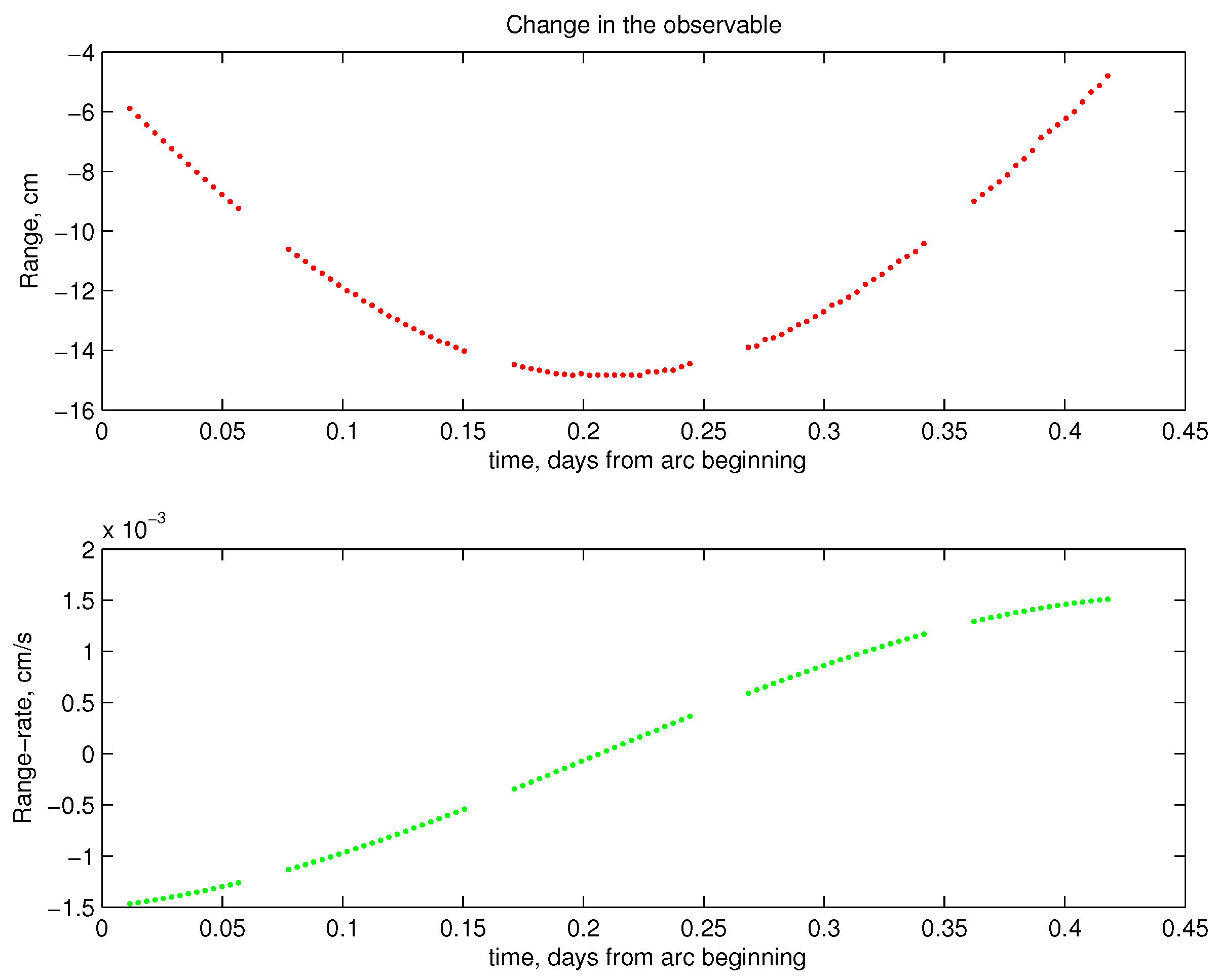
4.1. Observables Error Models

The observables we are dealing with are the tracking data (range and range-rate) and the non-gravitational accelerations, measured by the on-board accelerometer. To perform simulations in a realistic scenario, we need to properly add some measurement error to each observable.

4.1.1. Range and Range-Rate

According to [3], a nominal white noise can be associated to each tracking observation. Defining the simulated one-way range and range-rate observables as two-way measurements divided by 2 and assuming top accuracy performances of the transponder, we add a Gaussian error of ${\sigma }_r=23.7$ cm to the 120 s range observables and ${\sigma }_{\dot{r}}=8.7\times {10}^{-4}$ cm/s to the 30 s range-rate measurements [6]. These values represent the optimal performances in the $Ka$ band, while for the X band we assume 10 times larger errors.

From a comparison of the accuracies in the range and range-rate, it turns out that ${\sigma }_r/{\sigma }_{\dot{r}}\sim {10}^5$ s (according to Gaussian statistics, the standard deviations can be rescaled in order to be compared over the same integration time). Range measurements are, hence, more accurate than range-rate when we are observing phenomena with a period longer than ${10}^5$ s, while the opposite is true for range-rate. We can conclude that the relativity experiment, which involves long-term periodicity phenomena, is mainly performed through the range tracking data, while gravimetry and rotation experiments mainly with the range-rate (we recall that the Mercurycentric orbital period is less than ${10}^4$ s).

At the level of accuracy provided by the MORE relativity experiment, it could be necessary to account for additional sources of uncertainty in the range measurements. Indeed, instrumental related effects, such as residual signatures from the calibrator or residual biases after ground system calibration, can affect the observations in a non-negligible way. To account for these spurious effects, we add to the range Gaussian noise a generic systematic term, described by a bias of 3 cm and a sinusoidal trend (as already done in [12]) which reaches an amplitude of 3 cm after one year of observations. The choice of this functional behavior can be replaced by other assumptions, as done in [50]; it merely accounts for a possible scenario, which is the purpose of our simulations.

4.1.2. Accelerometer Readings and Calibration Strategy

As outlined in Section 3.3.5, we write the accelerometer contribution to the Mercurycentric motion of the spacecraft as ${\mathbf{a}}_{ISA}=-{\mathbf{a}}_{ng}+\mathbf{\epsilon }$, where ${\mathbf{a}}_{ng}$ is computed according to our simplified model. Concerning the error term ε, we assume the model provided by ISA team (private communications). It consists of a random background with some periodic terms superimposed: the main ones are a thermal term, resulting in a sinusoid at Mercury sidereal period ($7.6\times {10}^6$ s) and a resonant term, resulting in a sinusoid at the orbital period of the spacecraft ($8.3\times {10}^3$ s). All the details on the adopted model and the effects of the main components on the Mercurycentric orbit determination are described in [10].

The key issue in dealing with the accelerometer error term is that if we simply add it to the right hand side of the equation of motion, its detrimental effect causes a downgrading of the orbit determination of the spacecraft by orders of magnitude, vanifying the radio science experiment. In fact, this spurious instrumental effect is absorbed by the solve for parameters (like the state vector of the spacecraft at each arc) just like any other physical effect, resulting in a totally biased solution. To overcome this problem, the basic idea is to add to the right hand side of the equation of motion an additional term $c(\mathbf{\psi };t)$, function of a further set of parameters ψ, to be added in the solve for list, and of time, such that $\mathbf{\epsilon }(t)-c(\mathbf{\psi };t)\simeq 0$. In such a way, the calibration function $c(\mathbf{\psi };t)$ absorbs most of the accelerometer error and the physical parameters of interest for the radio science experiment are, in principle, not anymore biased. In the ORBIT14 software we implemented a novel calibration strategy, in which the calibration function is represented by a ${\mathcal{C}}^1$ cubic spline. All the details can be found in [19]. As a consequence, six additional parameters per arc (two per direction) are determined. We point out, as extensively discussed in [10], that this calibration strategy is able to absorb the low frequencies (i.e., longer than one day) error terms and the random component; in fact, the coefficients of the spline polynomials are computed once per arc, hence features with a periodicity lower than one day cannot be accounted for. This means that the resonant term, which shows a periodicity significantly lower than one day (about 2.3 h), is not absorbed by calibration at all. While this term results highly critical for what concerns the gravimetry and rotation experiments, we will see that its amplitude is not significantly detrimental for the relativity experiment.

4.2. Desaturation Maneuvres

Additional sources of perturbation on the orbit of the spacecraft around Mercury are the reaction wheels desaturation manoeuvres. We will assume as a general scenario to have one dump maneuvre during tracking and one dump maneuvre in the periods without tracking, hence a maximum amount of two dump manoeuvres per arc, as specified by the mission requirements. Each desaturation maneuvre, needed to maintain the desired attitude of the spacecraft, affects the precise Mercurycentric orbit determination. The result is a significant velocity change in the radial and out-of-plane directions and a linear momentum transfer in the transversal direction. To guarantee the expected level of accuracy in the orbit determination, these effects need to be modeled and removed from the estimation of the parameters. Each maneuvre appears in the spacecraft equation of motion as an additional acceleration acting on the probe. The downgrading effect on the spacecraft orbit determination can be significant, up to tens of meters in the range observations (see, e.g., [27]). For this reason, the velocity change $\Delta \mathbf{v}$ due to each maneuvre is added to the list of solve-for parameters, removing most of the downgrading effect from the orbit determination. The values for $\Delta \mathbf{v}$ adopted in simulations, along with all the details on the modelization and implementation of the maneuvres scenario, are given in [27]. The presence of orbital maneuvres, which are in general much larger than the desaturation maneuvres, is not considered here.

4.3. Metric Theories of Gravitation

A critical issue of the MORE relativity experiment, already discussed in [12], is that the Eddington parameter β and the Sun oblateness $J_{2\odot }$ show a near 1 correlation, as it appears from the covariance matrix obtained through the LS fit. This effect can be interpreted from a geometrical point of view considering that the main orbital effect of β is a precession of the argument of perihelion, which is a displacement taking place in the plane of the orbit of Mercury, while $J_{2\odot }$ affects the precession of the longitude of the node, thus producing a displacement in the plane of the solar equator. The angle between these two planes is only $\theta ={3.3}^{\circ }$, hence, being $cos\theta \simeq 1$, we can expect such a high correlation between the two parameters. The consequence is a significant deterioration of the formal accuracies of both parameters. Since, unavoidably, the geometrical configuration cannot be changed, a possible solution to determine both parameters without a significant loss in accuracy is to add a suitable constraint on one of the involved parameter. A meaningful possibility is to link the PN parameters through the Nordtvedt equation [51]:

$$\eta =4(\beta -1)-(\gamma -1)-{\alpha }_1-\frac{2}{3}{\alpha }_2.$$

In such a way, the knowledge on β is determined from the value of η: the correlation between β and η becomes almost 1, but that between β and $J_{2\odot }$ is greatly reduced. The introduction of the Nordtvedt equation is justified if we assume that gravitation must be described by a metric theory. In the following this becomes a basic assumption of our scenario.

4.4. Rank Deficiencies in the Mercury and EMB Orbit Determination Problem

As already stated, to perform the MORE relativity experiment we need to determine the orbit of Mercury and the EMB, that is to compute their state vector (position and velocity) at a given reference epoch. In practice, we find that we cannot solve for all the 12 components of the 2 state vectors without running into a significant deterioration of the results. The issue arises from the fact that this orbit determination problem, including simultaneously Mercury and the Earth, shows an approximate rank deficiency of order 4 (see, e.g., [12] for details).

An approximate rank deficiency of order 3 results from the breaking of an exact symmetry of the problem with respect to the full rotation group $SO(3)$. If there were only the Sun, the Earth and Mercury and if the Sun was exactly spherically symmetric (i.e., $J_{2\odot }=0$), there would be an exact symmetry for rotation in determining both the orbits of Mercury and the Earth and therefore an exact rank deficiency of order 3. Due to the coupling with the other planets and to the asphericity of the Sun, the exact symmetry is broken but only by a small parameter (of the order of the relative size of the mutual perturbations by the other planets on the orbits of Mercury and the Earth and of the size of $J_{2\odot }$), bringing a residual approximate rank deficiency of order 3 in the problem.

A further exact symmetry would be present, if there were only the Sun, the Earth and Mercury. Changing all the lengths by a factor L, all the masses by a factor M and all the time intervals by a factor T, provided that the scaling factors are related by $L^3=T^{2}M$ (Kepler’s third law), the equation of motion of the gravitational 3-body problem would remain unchanged. Again, this symmetry is broken by a small parameter, and an approximate rank deficiency of order 1 remains, leading to a total rank deficiency of order 4.

The standard solution already adopted in [12] is to solve for only 8 of the 12 components of the state vectors, assuming the remaining 4 as consider parameters. In the following we adopt the same assumption and we do not solve for the three position components of the EMB orbit ($x_{EM},y_{EM},z_{EM}$) and for the EMB velocity component perpendicular to the EMB orbital plane (${\dot{z}}_{EM}$). The adopted technique is called descoping. A different approach to a problem of rank deficiency of order d is to add d constraint equations as apriori observations, instead of removing d parameters from the solve for list (see [25]—Chapter 6 for details). This is the technique we apply, for example, assuming the validity of the Nordtvedt equation in order to remove the degeneracy between β and $J_{2\odot }$. In ORBIT14 we have implemented also the possibility of determining all the 12 state vectors components, by adding 4 apriori constraints between the state vectors components and the Sun’s mass ${\mu }_{\odot }$ in order to remove the degeneracy. A detailed discussion on this topic will be presented in a future paper by our group. In the following we assume to determine only 8 out of the 12 components.

5. Results

In this Section we will present and discuss the results of our simulations. In this review, we are mainly interested in the MORE relativity experiment: the results concerning PN and related parameters will be given in Section 5.1. For completeness, we will discuss the results concerning gravimetry and rotation in Section 5.2.

At each iteration of the differential correction process we solve for the following parameters:

• Global dynamical:

  -

  PN parameters: β, γ, η, ${\alpha }_1$, ${\alpha }_2$;

  -

  other parameters of interest for the relativity experiment: ${\mu }_{\odot }$, ζ, $J_{2\odot }$;

  -

  the state vectors of Mercury and EMB (8 components): ($x_M,y_M,z_M;{\dot{x}}_M,{\dot{y}}_M,{\dot{z}}_M$); (${\dot{x}}_{EM},{\dot{y}}_{EM}$);

  -

  normalized harmonic coefficients of the gravity field of Mercury up to degree and order 25 and the Love number $k_2$;

  -

  rotational parameters: ${\delta }_1$, ${\delta }_2$, ${\epsilon }_1$, ${\epsilon }_2$;

  -

  six accelerometer calibration coefficients for each arc, plus 6+6 boundary conditions;

• Local dynamical:

  -

  state vector of the Mercurycentric orbit of the spacecraft, in the Ecliptic J2000 inertial reference frame, at the central time of each observed arc;

  -

  three dump manoeuvre components, $\Delta \mathbf{v}$, taking place during tracking, for each observed arc;

• External local dynamical:

  -

  three dump manoeuvre components, $\Delta \mathbf{v}$, taking place in the period without tracking between each pair of consecutive observed arcs.

5.1. The Relativity Experiment Results

The results for the PN and related parameters of interest for the relativity experiment are shown in

Table 1. Simulation results for the parameters of interest in the MORE relativity experiment (errors on ${\mu }_{\odot }$ are in cm${}^3$/s${}^2$, on ζ in y${}^{-1}$).

Parameter	Formal Error	True Error	T/F Error Ratio	Current Accuracy
β	$7.3\times {10}^{-7}$	$2.6\times {10}^{-6}$	3.6	$7\times {10}^{-5}$ [52]
γ	$9.3\times {10}^{-7}$	$1.1\times {10}^{-6}$	1.2	$2.3\times {10}^{-5}$ [48]
η	$2.2\times {10}^{-6}$	$1.1\times {10}^{-5}$	4.9	$4.5\times {10}^{-4}$ [53]
${\alpha }_1$	$4.9\times {10}^{-7}$	$4.9\times {10}^{-7}$	1.0	$6.0\times {10}^{-6}$ [54]
${\alpha }_2$	$8.3\times {10}^{-8}$	$1.0\times {10}^{-7}$	1.2	$3.5\times {10}^{-5}$ [54]
${\mu }_{\odot }$	$4.2\times {10}^{13}$	$4.2\times {10}^{13}$	1.0	${10}^{16}$, $8\times {10}^{15}$ [55,56]
ζ	$2.3\times {10}^{-14}$	$3.6\times {10}^{-14}$	1.5	$4.3\times {10}^{-14}$ [57]
$J_{2\odot }$	$4.1\times {10}^{-10}$	$4.1\times {10}^{-10}$	1.0	$1.2\times {10}^{-8}$ [52]

. For each parameter we report the following quantities: (i) the formal uncertainty; (ii) the true error; (iii) the true-to-formal (T/F) error ratio; (iv) the current accuracy with which the parameter is presently known.

The formal error is obtained from the diagonal terms of the covariance matrix. The main limitation of formal analysis is that it does not account at all for any error that is non-Gaussian, like systematic errors, or time-correlated, unless they are in some way calibrated introducing further parameters in the solve-for list. Besides the formal analysis, we introduce a second quantity, which we call “true” error, to assess the expected accuracies in a more realistic way. This quantity is defined for each parameter as the difference between the nominal value of the parameter (used in simulations) and the value determined at convergence of the differential correction process. In such a way, the systematic effects are included in the computation of the accuracies. The true errors shown in Table 1 have been obtained as rms values over a number of runs carried out by changing the seed of the random numbers generator. We found that ∼10 runs are adequately representative to quantify systematic errors. The ideal situation would occur when T/F error ratios follow Gaussian statistics, which means either that no systematic effects are present at all or that they are accounted for, through calibration parameters, in the formal analysis. In practice, this ratio is almost always greater than 1, but what does matter is that it is limited within a maximum of T/F$\sim$ 3. Any higher value would be representative of a wrong or lacking modelization of some effects.

Analyzing the two sources of systematic effects included in simulation, i.e., the error model for accelerometer readings and the spurious effects from the ranging system, we found that T/F values higher than 1 for the relativity parameters can be only partially ascribed to non-perfectly calibrated long term components in the accelerometer error model, which are not fully absorbed by the ${\mathcal{C}}^1$ spline calibration. The main downgrading effect turns out to be the presence of systematic terms in the range error model, which are not calibrated at all. The effect is particularly detrimental for the determination of β and η. We remind that the range error model includes a bias term of 3 cm and a sinusoidal trend up to 3 cm after one year. Analyzing individually the two error terms, we found that the bias term is responsible for most of the deterioration in estimating β and η. Adding the linear term does not further deteriorate true errors in a significant way. Moreover, as extensively discussed in [50], increasing the adopted value for the bias term results in a corresponding increase of the true errors of all the PN parameters.

A possible approach to the problem would be to introduce in the solve-for list an additional global parameter, that is a bias in modeling the range observables. Estimating the bias, it could be possible in principle to absorb most of the spurious effect in range, leading to a better estimate of the PN parameters in terms of T/F error ratios. This approach has a disadvantage that immediately appears when we take correlations into account. The correlations between PN and related parameters are shown in

Table 2. Correlations between PN and related parameters (values higher than 0.7 are highlighted in bold).

	β	γ	η	${\mathit{\alpha }}_1$	${\mathit{\alpha }}_2$	${\mathit{\mu }}_{\odot }$	ζ	${\mathit{J}}_{2\odot }$
$J_{2\odot }$	0.15	0.21	0.11	0.90	0.29	0.89	0.10	–
ζ	<0.1	0.28	<0.1	<0.1	0.17	<0.1	–
${\mu }_{\odot }$	0.20	0.14	0.14	0.84	<0.1	–
${\alpha }_2$	0.35	0.28	0.36	0.27	–
${\alpha }_1$	0.35	0.12	0.22	–
η	0.96	0.60	–
γ	0.77	–
β	–

. As expected, the correlation between β and η is almost one. In fact we adopted the Nordvedt relation as an apriori constraint between PN parameters and we included an apriori constraint on γ from the SCE simulations during cruise phase. As a consequence, η is deduced from β and their correlation is very high. If we add a bias in range to the solve-for list, the correlation between the bias term and, especially, β and η turns out to be almost one. This would lead to a worsening in the formal error of both β and η by more than one order of magnitude. This result would not be compliant with the scientific goals expected from MORE in terms of accuracies. In fact, the goal is to determine η at a level of, at least, ${10}^{-5}$ and β at a level of some parts in ${10}^{-6}$ [3,6,12]. In conclusion, if the systematic effects due to the ranging system remain at the level of few cm, the downgrading effect on the accuracies is still acceptable, as can be envisaged comparing the present results with current accuracies. Conversely, if the systematic terms, especially a spurious bias in the range measurements, become more significant, some suitable calibration strategy would be mandatory. As sketched in Section 4.4, the different approach of estimating all the 12, instead of only 8, components of Mercury and the EMB state vectors by adding some apriori constraints is under analysis. Preliminary attempts have shown that in such a case the correlation between the bias term in range and η and β would significantly decrease. We will report our conclusions in a future work.

A critical issue in the MORE relativity experiment, already remarked in [12] (p. 17), concerns the effects of a lacking knowledge of the Solar System model. In our simulations, we assumed that all the parameters of the SS model not included in the solve-for list (for example, the masses of the planets) are known from the ephemerides well enough that no spurious effects are introduced in the parameters estimation. An extensive discussion on this approximation has been carried out in [31] and the issue is still controversial.

Finally, we point out that the Lense-Thirring effect on the Mercury’s orbit due to the Sun’s angular momentum has been neglected. This choice has presently been made in order to simplify the development and implementation of the dynamical models. However, the effect is expected to be relevant [58], hence in future work we will investigate on its possible impact on the relativity parameters determination.

5.2. Results for Gravimetry and Rotation

In Section 4.1.1, we introduced one of the basic issues of the BepiColombo radio science experiment. Comparing the expected accuracies of range and range-rate, it turns out that range-rate measurements are more accurate than range data when observing phenomena with periodicity shorter than ∼${10}^5$ s, while the opposite is true for long-term periodicity phenomena. As a consequence, gravimetry and rotation experiments are mainly performed by means of range-rate data, while the relativity experiment by means of range. MORE is a comprehensive experiment in which all the parameters are solved simultaneously in the non-linear LS fit, but the expected independence between gravimetry/rotation on one side and relativity on the other suggests that, for the purpose of simulations, we can perform the experiments individually or all together and achieve the same results. We checked the validity of this statement by performing additional simulations. Referring to the solve-for list in Section 4, we ran the following simulations:

• relativity simulations: we removed from the solve-for list the gravimetry and rotational parameters, i.e. the gravity field spherical harmonic coefficients, Love number $k_2$, the angles $({\delta }_1,{\delta }_2)$, the libration amplitudes ${\epsilon }_1$, ${\epsilon }_2$;
• gravimetry and rotation simulations: we removed from the solve-for list the PN and related parameters.

These are mandatory tests since the chance that any further unforeseen rank deficiency between relativity and gravimetry/rotation parameters appears in the global fit needs to be verified. The results confirmed our expectations. The accuracies of PN and related parameters achieved in the global simulation, discussed in Section 5.1, and in the relativity simulations are equivalent, and the same is true for gravimetry and rotation. We have already extensively reported in [10] on the results for the MORE gravimetry and rotation experiments, together with a discussion on the achievable accuracy in the orbit determination. Therefor, we do not duplicate here the same results and we refer to that paper for a discussion on these topics. We point out that in the simulations described here we did not include among the observables the optical data from the high resolution camera HRIC, part of the SIMBIO-SYS payload [59]. In fact, camera observations significantly support range-rate measurements in the determination of the rotational parameters, while they do not contribute at all to the relativity experiment.

6. Discussion and Conclusions

In this review, we summarized all the issues concerning the BepiColombo relativity experiment. After recalling the global structure of the ORBIT14 software and the techniques to determine the parameters of interest, we detailed the essential mathematical models on which the experiment is based and the fundamental assumptions adopted. We finally presented the results of a full cycle of simulations carried out in the latest mission scenario.

At the beginning of 2000’s our group performed a similar set of simulations, whose results are reported in [12], with the specific aim of dictating the mission and instrumentation requirements in order to make the BepiColombo relativity experiment feasible. Several underlying issues concerning the experiment have since been reconsidered and updated and the software has undergone significant revision. The formal results of the present paper are compared with the formal errors obtained in 2002 in [12] in

Table 3. Comparison between the results in Schettino & Tommei (2016) (this paper) and previous results of the relativity experiment (${\mu }_{\odot }$ in cm${}^3$/s${}^2$).

Parameter	Schettino & Tommei (2016)	Milani et al. (2002) [12]	Iess et al. (2009) [6]
β	$7.3\times {10}^{-7}$	$9.2\times {10}^{-7}$	$2\times {10}^{-6}$
γ	$9.3\times {10}^{-7}$	$2\times {10}^{-6}$ (SCE)	$2\times {10}^{-6}$
η	$2.2\times {10}^{-6}$	$3.3\times {10}^{-6}$	$8\times {10}^{-6}$
${\alpha }_1$	$4.9\times {10}^{-7}$	$7.1\times {10}^{-7}$	–
${\alpha }_2$	$8.3\times {10}^{-8}$	$1.9\times {10}^{-7}$	–
${\mu }_{\odot }$	$4.2\times {10}^{13}$	$4.1\times {10}^{13}$	–
$J_{2\odot }$	$4.1\times {10}^{-10}$	$6.2\times {10}^{-10}$	$2\times {10}^{-9}$

, where the results reported in [6], representing the goal accuracies required for the MORE relativity experiment, have also been included. We refer to Experiment D in [12], where Nordtvedt equation has been assumed to link PN parameters. In the comparison we did not consider the ζ parameter because in [12] the quantity $\dot{G}/G$ was included instead of ζ.

It can be seen that a slight improvement of the 2002 expectations [12] has been achieved. It can be remarked that in both cases formal errors turn out to be significantly lower than the goal accuracies of MORE. A quantitative comparison with the 2015 results in [15] is difficult because the mission time span scenario is different and, furthermore, the assumption of a metric theory of gravitation was not included in [15].

At this stage, the spacecraft is almost ready for launch and no significant modification of the mission can be addressed anymore. The aim of the set of simulations described in this review is, hence, clear: assuming the performances expected and tested for each instrument and the revised launch scenario, we want to establish the feasibility of the relativity experiment and provide the results that can be achieved in terms of accuracies. Two key issues were pointed out already during the past years: the impact on the solution from the errors in the accelerometer readings and from the aging of the transponder. Concerning the first issue, the main downgrading source was found in the thermal effects which produce periodic spurious signatures, with the periodicity of both the orbital period of the spacecraft around Mercury and the sidereal period of Mercury around the Sun. These signatures mainly affect the Mercurycentric orbit determination. An extensive discussion on the potentially downgrading effects for the gravimetry and rotation experiments have been recently discussed by our group in [10]. The results shown in Table 1 and the discussions presented in [14,50] lead us to the conclusion that, if the accelerometer error model is compliant to the one adopted, the effects on the relativity experiment are not detrimental. More critical is the question on how the ranging system affects the results. In [12] it was shown that, describing the transponder aging with a sinusoidal trend up to some tens of cm after one year, the effect was highly detrimental for the relativity parameters estimation. This issue has been tackled by introducing an on-board calibrator to account for the aging of the transponder. Nevertheless, residual spurious effects due, e.g., to the calibrator itself or to the on-ground instrumentation can still lead to a systematic error of a few cm. In our simulations, we assumed a bias of 3 cm and a sinusoidal trend up to 3 cm after one year. In such a case, the detrimental effects on the parameters are restrained, but in an unfavorable scenario in which they exceed the value of 5 cm on the one-way range, the solution would be significantly downgraded, as shown in [50]. In such a case, we envisage the need of a calibration strategy within the LS fit. In any case, in the realistic scenario presented here, we can conclude that the accuracies achievable by the BepiColombo relativity experiment for each of the PN parameter, compared with current accuracies, would represent a significant improvement of our knowledge of gravitational theories.

References

1. Benkhoff, J.; van Casteren, J.; Hayakawa, H.; Fujimoto, M.; Laakso, H.; Novara, M.; Ferri, P.; Middleton, H.R.; Ziethe, R. BepiColombo-Comprehensive exploration of Mercury: Mission overview and science goals. Planet. Space Sic. 2010, 58, 2–20. [Google Scholar] [CrossRef]
2. Mukai, T.; Yamakawa, H.; Hayakawa, H.; Kasaba, Y.; Ogawa, H. Present status of the BepiColombo/Mercury magnetospheric orbiter. Adv. Space Res. 2006, 38, 578–582. [Google Scholar] [CrossRef]
3. Iess, L.; Boscagli, G. Advanced radio science instrumentation for the mission BepiColombo to Mercury. Planet. Space Sci. 2001, 49, 1597–1608. [Google Scholar] [CrossRef]
4. Milani, A.; Rossi, A.; Vokrouhlický, D.; Villani, D.; Bonanno, C. Gravity field and rotation state of Mercury from the BepiColombo Radio Science Experiments. Planet. Space Sci. 2001, 49, 1579–1596. [Google Scholar] [CrossRef]
5. Sanchez Ortiz, N.; Belló Mora, M.; Jehn, R. BepiColombo mission: Estimation of Mercury gravity field and rotation parameters. Acta Astronaut. 2006, 58, 236–242. [Google Scholar] [CrossRef]
6. Iess, L.; Asmar, S.; Tortora, P. MORE: An advanced tracking experiment for the exploration of Mercury with the mission BepiColombo. Acta Astronaut. 2009, 65, 666–675. [Google Scholar] [CrossRef]
7. Genova, A.; Marabucci, M.; Iess, L. Mercury radio science experiment of the mission BepiColombo. Mem. Soc. Astron. Ital. Suppl. 2012, 20, 127–132. [Google Scholar]
8. Schettino, G.; Di Ruzza, S.; De Marchi, F.; Cicalò, S.; Tommei, G.; Milani, A. The radio science experiment with BepiColombo mission to Mercury. Mem. Soc. Astron. Ital. 2016, 87, 24–29. [Google Scholar]
9. Cicalò, S.; Milani, A. Determination of the rotation of Mercury from satellite gravimetry. Mon. Not. R. Astron. Soc. 2012, 427, 468–482. [Google Scholar] [CrossRef]
10. Cicalò, S.; Schettino, G.; Di Ruzza, S.; Alessi, E.M.; Tommei, G.; Milani, A. The BepiColombo MORE gravimetry and rotation experiments with the ORBIT14 software. Mon. Not. R. Astron. Soc. 2016, 457, 1507–1521. [Google Scholar] [CrossRef]
11. Palli, A.; Bevilacqua, A.; Genova, A.; Gherardi, A.; Iess, L.; Meriggiola, R.; Tortora, P. Implementation of an End to End Simulator for the BepiColombo Rotation Experiment. In Proceedings of the European Planetary Space Congress 2012, Madrid, Spain, 23–28 September 2012.
12. Milani, A.; Vokrouhlicky, D.; Villani, D.; Bonanno, C.; Rossi, A. Testing general relativity with the BepiColombo Radio Science Experiment. Phys. Rev. D 2002, 66. [Google Scholar] [CrossRef]
13. Milani, A.; Tommei, G.; Vokrouhlicky, D.; Latorre, E.; Cicalò, S. Relativistic models for the BepiColombo radioscience experiment. In Relativity in Fundamental Astronomy: Dynamics, Reference Frames, and Data Analysis; Cambridge University Press: Cambridge, UK, 2010. [Google Scholar]
14. Schettino, G.; Cicalò, S.; Di Ruzza, S.; Tommei, G. The relativity experiment of MORE: Global full-cycle simulation and results. In Proceedings of the IEEE Metrology for Aerospace (MetroAeroSpace), Benevento, Italy, 4–5 June 2015; pp. 141–145.
15. Schuster, A.K.; Jehn, R.; Montagnon, E. Spacecraft design impacts on the post-Newtonian parameter estimation. In Proceedings of the IEEE Metrology for Aerospace (MetroAeroSpace), Benevento, Italy, 4–5 June 2015; pp. 82–87.
16. Tommei, G.; De Marchi, F.; Serra, D.; Schettino, G. On the Bepicolombo and Juno Radio Science Experiments: Precise models and critical estimates. In Proceedings of the IEEE Metrology for Aerospace (MetroAeroSpace), Benevento, Italy, 4–5 June 2015; pp. 323–328.
17. Kaula, W.M. Theory of Satellite Geodesy: Applications of Satellites to Geodesy; Blaisdell: Waltham, MA, USA, 1996. [Google Scholar]
18. Kozai, Y. Effects of the tidal deformation of the Earth on the motion of close Earth satellites. Publ. Astron. Soc. Jpn. 1965, 17, 395–402. [Google Scholar]
19. Alessi, E.M.; Cicalò, S.; Milani, A. Accelerometer data handling for the BepiColombo orbit determination. In Advances in the Astronautical Science, Proccedings of the 1st IAA Conference on Dynamics and Control of Space Systems, Porto, Portugal, 19–21 March 2012.
20. Iafolla, V.; Nozzoli, S. Italian Spring Accelerometer (ISA): A high sensitive accelerometer for BepiColombo ESA Cornerstone. Planet. Space Sci. 2001, 49, 1609–1617. [Google Scholar] [CrossRef]
21. Will, C.M. Theory and Experiment in Gravitational Physics; Cambridge University Press: Cambridge, UK, 1993. [Google Scholar]
22. Tommei, G.; Milani, A.; Vokrouhlicky, D. Light-time computations for the BepiColombo Radio Science Experiment. Celest. Mech. Dyn. Astron. 2010, 107, 285–298. [Google Scholar] [CrossRef]
23. Mazarico, E.; Genova, A.; Goossens, S.; Lemoine, F.G.; Neumann, G.A.; Zuber, M.T.; Smith, D.E.; Solomon, S.C. The gravity field, orientation, and ephemeris of Mercury from MESSENGER observations after three years in orbit. J. Geophys. Res. 2014, 119, 2417–2436. [Google Scholar] [CrossRef]
24. Jehn, R.; Rocchi, A. BepiColombo Mercury Cornerstone Mission Analysis: The April 2018 Launch Option. MAS Working Paper No. 608; BC-ESC-RP-50013; 24 March 2016; Issue 2.1. Available online: http://issfd.org/ISSFD_2014/ISSFD24_Paper_S6-5_jehn.pdf (accessed on 5 August 2016).
25. Milani, A.; Gronchi, G.F. Theory of Orbit Determination; Cambridge University Press: Cambridge, UK, 2010. [Google Scholar]
26. Folkner, W.M.; Williams, J.G.; Boggs, D.H. The Planetary and Lunar Ephemeris DE 421; JPL Publication: Pasadena, CA, USA, 2008. [Google Scholar]
27. Alessi, E.M.; Cicalò, S.; Milani, A.; Tommei, G. Desaturation Manoeuvres and Precise Orbit Determination for the BepiColombo Mission. Mon. Not. R. Astron. Soc. 2012, 423, 2270–2278. [Google Scholar] [CrossRef]
28. Bonanno, C.; Milani, A. Symmetries and rank deficiency in the orbit determination around another planet. Celest. Mech. Dyn. Astron. 2002, 83, 17–33. [Google Scholar] [CrossRef]
29. Will, C.M. The Confrontation between General Relativity and Experiment. Living Rev. Relativ. 2014, 17, 1–117. [Google Scholar] [CrossRef]
30. Shapiro, I.I. Fourth Test of General Relativity. Phys. Rev. Lett. 1964, 13, 789–791. [Google Scholar] [CrossRef]
31. De Marchi, F.; Tommei, G.; Milani, A.; Schettino, G. Constraining the Nordtvedt parameter with the BepiColombo Radioscience experiment. Phys. Rev. D 2016, 93, 123014. [Google Scholar] [CrossRef]
32. Peebles, P.J.E. Principles of Physical Cosmology; Princeton University Press: Princeton, NJ, USA, 1993. [Google Scholar]
33. Klioner, S.A. Relativistic scaling of astronomical quantities and the system of astronomical units. Astron. Astrophys. 2008, 478, 951–958. [Google Scholar] [CrossRef]
34. Klioner, S.A.; Capitaine, N.; Folkner, W.; Guinot, B.; Huang, T.Y.; Kopeikin, S.; Petit, G.; Pitjeva, E.; Seidelmann, P.K.; Soffel, M. Units of Relativistic Time Scales and Associated Quantities. In Relativity in Fundamental Astronomy: Dynamics, Reference Frames, and Data Analysis; Cambridge University Press: Cambridge, UK, 2010. [Google Scholar]
35. Moyer, T.D. Formulation for Observed and Computed Values of Deep Space Network Data Types for Navigation, NASA-JPL, Deep Space Communication and Navigation Series, Monograph 2; John Wiley & Sons: Hoboken, NJ, USA, 2000. [Google Scholar]
36. Soffel, M.; Klioner, S.A.; Petit, G.; Wolf, P.; Kopeikin, S.M.; Bretagnon, P.; Brumberg, V.A.; Capitaine, N.; Damour, T.; Fukushima, T. The IAU Resolutions for Astrometry, Celestial Mechanics, and Metrology in the Relativistic Framework: Explanatory Supplement. Astron. J. 2003, 126, 2687–2706. [Google Scholar] [CrossRef]
37. Irwin, A.W.; Fukushima, T. A numerical time ephemeris of the Earth. Astron. Astrophys. 1999, 348, 642–652. [Google Scholar]
38. Damour, T.; Soffel, M.; Hu, C. General-relativistic celestial mechanics. IV. Theory of satellite motion. Phys. Rev. D 1994, 49, 618–635. [Google Scholar] [CrossRef]
39. Archinal, B.A.; A’Hearn, M.F.; Bowell, E.; Conrad, A.; Consolmagno, G.J.; Courtin, R.; Fukushima, T.; Hestroffer, D.; Hilton, J.L.; Krasinskyet, G.A.; et al. Report of the IAU Working Group on Cartographic Coordinates and Rotational Elements: 2009. Celest. Mech. Dyn. Astron. 2011, 2, 101–135. [Google Scholar] [CrossRef]
40. Montenbruck, O.; Gill, E. Satellite Orbits: Models, Methods and Applications; Springer: Berlin, Germany, 2005. [Google Scholar]
41. Padovan, S.; Margot, J.-L.; Hauck, S.A., II; Moore, W.B.; Solomon, S.C. The tides of Mercury and possible implications for its interior structure. J. Geophys. Res. 2014, 119, 850–866. [Google Scholar] [CrossRef]
42. Roy, A.E. Orbital Motion, 4th ed.; CRC Press: Boca Raton, FL, USA, 2005. [Google Scholar]
43. Peale, S.J. The Rotational Dynamics of Mercury and the State of Its Core; University Arizona press: Tucson, AZ, USA, 1988; pp. 461–493. [Google Scholar]
44. Peale, S.J. The proximity of Mercury’s spin to Cassini state 1 from adiabatic invariance. Icarus 2006, 181, 338–347. [Google Scholar] [CrossRef]
45. Yseboodt, M.; Margot, J.L.; Peale, S.J. Analytical model of the long-period forced longitude librations of Mercury. Icarus 2010, 207, 536–544. [Google Scholar] [CrossRef]
46. Yseboodt, M.; Rivoldini, A.; Van Hoolst, T.; Dumberry, M. Influence of an inner core on the long-period forced librations of Mercury. Icarus 2013, 226, 41–51. [Google Scholar] [CrossRef]
47. Stark, A.; Oberst, J.; Preusker, F.; Peale, S.J.; Margot, J.-L.; Phillips, R.J.; Neumann, G.A.; Smith, D.E.; Zuber, M.T.; Solomon, S.C. First MESSENGER orbital observations of Mercury’s librations. Geophys. Res. Lett. 2015, 42, 7881–7889. [Google Scholar] [CrossRef]
48. Bertotti, B.; Iess, L.; Tortora, P. A test of general relativity using radio links with the Cassini spacecraft. Nature 2003, 425, 374–376. [Google Scholar] [CrossRef] [PubMed]
49. Imperi, L.; Iess, L. Testing general relativity during the cruise phase of the BepiColombo mission to Mercury. In Proceedings of the IEEE Metrology for Aerospace (MetroAeroSpace), Benevento, Italy, 4–5 June 2015.
50. Schettino, G.; Imperi, L.; Iess, L.; Tommei, G. Sensitivity study of systematic errors in the BepiColombo relativity experiment. In Proceedings of the Metrology for Aerospace (MetroAeroSpace), Florence, Italy, 22–23 June 2016. in press.
51. Nordtvedt, K.J. Post-Newtonian Metric for a General Class of Scalar-Tensor Gravitational Theories and Observational Consequences. Astrophys. J. 1970, 161, 1059–1067. [Google Scholar] [CrossRef]
52. Fienga, A.; Laskar, J.; Exertier, P.; Manche, H.; Gastineau, M. Numerical estimation of the sensitivity of INPOP planetary ephemerides to general relativity parameters. Celest. Mech. Dyn. Astron. 2015, 123, 325–349. [Google Scholar] [CrossRef]
53. Williams, J.G.; Turyshev, S.G.; Boggs, D.H. Lunar Laser Ranging Tests of the Equivalence Principle with the Earth and Moon. Int. J. Mod. Phys. D 2009, 18, 1129–1175. [Google Scholar] [CrossRef]
54. Iorio, L. Constraining the Preferred-Frame α1, α2 Parameters from Solar System Planetary Precessions. Int. J. Mod. Phys. D 2014, 23, 1450006. [Google Scholar] [CrossRef]
55. Pitjeva, E.V. Determination of the Value of the Heliocentric Gravitational Constant (GM) from Modern Observations of Planets and Spacecraft. J. Phys. Chem. Ref. Data 2015, 44, 031210. [Google Scholar] [CrossRef]
56. The Value has Been Obtained from Latest JPL Ephemerides and Has Been Published on the NASA HORIZONS Web-Interface. Available online: http://ssd.jpl.nasa.gov/?constants (accessed on 5 August 2016).
57. Pitjeva, E.V.; Pitjev, N.P. Relativistic effects and dark matter in the Solar system from observations of planets and spacecraft. Mon. Not. R. Astron. Soc. 2013, 432, 3431–3437. [Google Scholar] [CrossRef]
58. Iorio, L.; Lichtenegger, H.I.M.; Ruggiero, M.L.; Corda, C. Phenomenology of the Lense-Thirring effect in the solar system. Astrophys. Space Sci. 2011, 331, 351–395. [Google Scholar] [CrossRef]
59. Flamini, E.; Capaccioni, F.; Colangeli, L.; Cremonese, G.; Doressoundiram, A.; Josset, J.L.; Langevin, L.; Debei, S.; Capria, M.T.; De Sanctis, M.C.; et al. SIMBIO-SYS: The spectrometer and imagers integrated observatory system for the BepiColombo planetary orbiter. Planet. Space Sci. 2010, 58, 125–143. [Google Scholar] [CrossRef]
Figure 1. Block diagram of the ORBIT14 code: simulation and differential corrections stages. Green arrows refer to simulator inputs/outputs and orange arrows to corrector inputs/outputs. The input option files for simulator and corrector are similar and include, for example, the state vector of the spacecraft at the initial epoch, the number of considered arcs, the time steps for the orbit propagation of the spacecraft, Mercury and EMB, the time sampling for range, range-rate and accelerometer data.
Universe 02 00021 g001
Figure 2. Block diagram of a differential corrector decomposed in three steps: (1) in “cor_par_setup” all the input options are read, data are split for the following parallel computation and the orbits of Mercury and EMB are propagated; (2) “cor_par_arc” contains most of the computationally expensive processing and is parallelized, by executing multiple copies of the same code, without need for interprocess communication; at this stage, the orbit of the spacecraft is propagated at each arc, the light-time computation is performed and residuals and normal matrix are given as output for the next step; (3) in “cor_solve” the covariance matrix and the LS solution are computed.
Universe 02 00021 g002
Figure 3. Schematic representation of observed and extended arc. The times t i ( i = 1 , . . , 4 ) are the central epoch of each arc; the black bars correspond to dark intervals, without tracking from Earth. See the text for more explanation.
Universe 02 00021 g003
Figure 4. Vectors involved in the multiple dynamics for the tracking of the spacecraft from the Earth.
Universe 02 00021 g004
Figure 5. The difference in the observables range and range-rate for one pass of Mercury above the horizon for a ground station, by using an hybrid model in which the position and velocity of the orbiter have not been transformed to TDB-compatible quantities and a correct model in which all quantities are TDB-compatible. Gaps of the signal are due to spacecraft passage behind Mercury as seen for the Earth station. (Top): for a hybrid model with the satellite position and velocity not transformed to TDB-compatible; (Bottom): for a hybrid model with the position and velocity of the antenna not transformed to TDB-compatible.
Universe 02 00021 g005aUniverse 02 00021 g005b