Testing [O ii] λ3727 as a Star Formation Rate Tracer in Quasar Host Galaxies

 , , , , and
Abstract
1. Introduction
2. Sample
2.1. Sample Selection
2.2. Reference FIR Star Formation Rates
3. Spectroscopic Observations and Measurements
3.1. [O ii] Measurements for the SDSS Quasar Sample
3.2. [O ii] Measurements for the PG Quasar Sample and Observations
3.3. [O ii] Star Formation Rates
3.4. Robustness of the Emission-Line Measurements
4. Comparison Between [O ii] and FIR Star Formation Rates
4.1. Comparison Results
4.2. Dependence of the SFR Offset on AGN Activity
4.3. Dependence of the SFR Offset on Redshift
4.4. Sensitivity to the Adopted AGN NLR Correction
5. Summary and Conclusions
- 1.
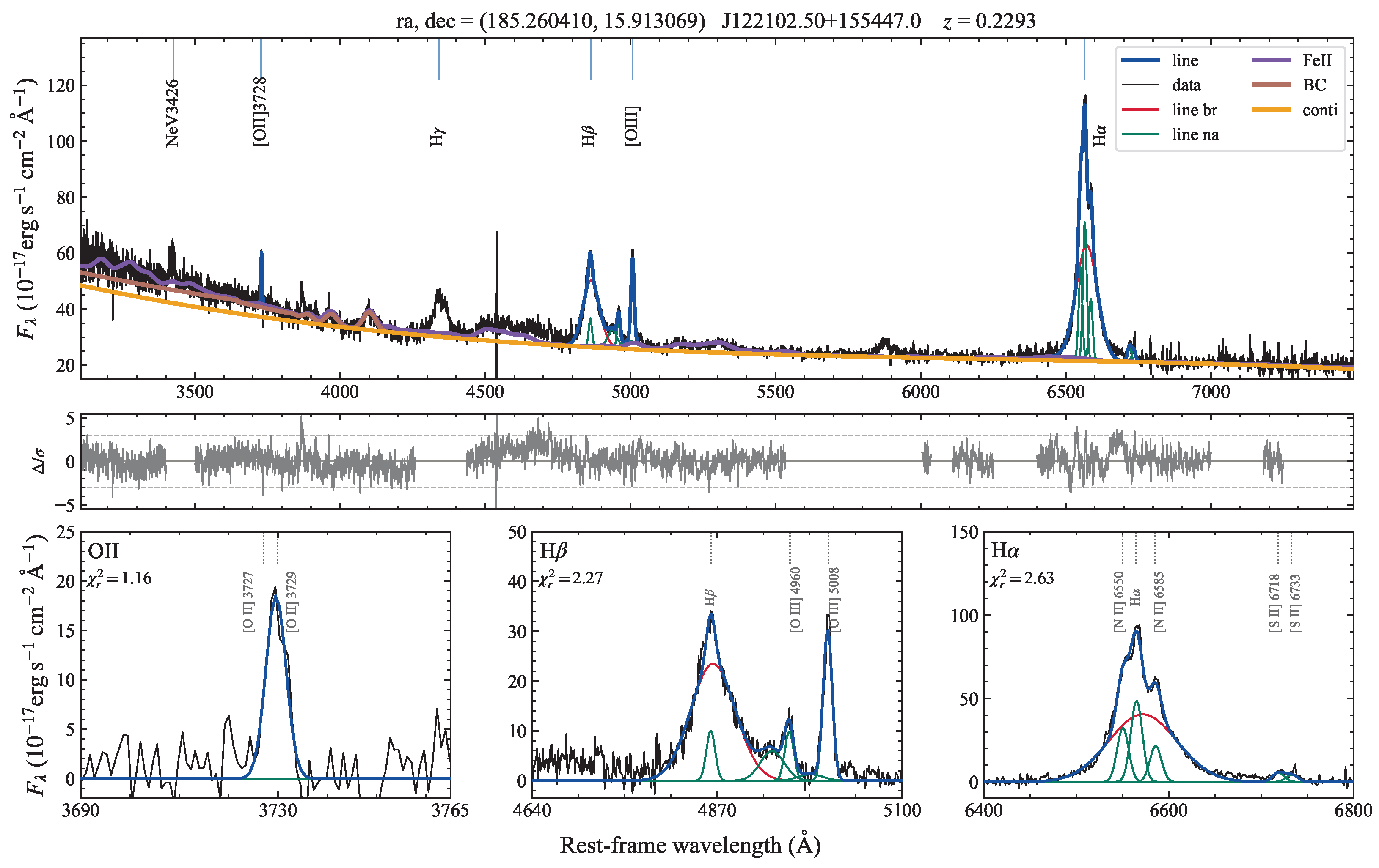
- We refit the SDSS spectra of 120 SDSS quasars and 31 PG quasars with available SDSS spectra using QSOFITMORE. For the remaining PG quasars without suitable archival spectra, we obtained new optical spectroscopic observations with XLT, LJT, HCT, and P200/DBSP. We got new spectra for 52 PG quasars. These spectra-fitting results provide the narrow emission line luminosities for calculating [O ii] SFRs.
- 2.
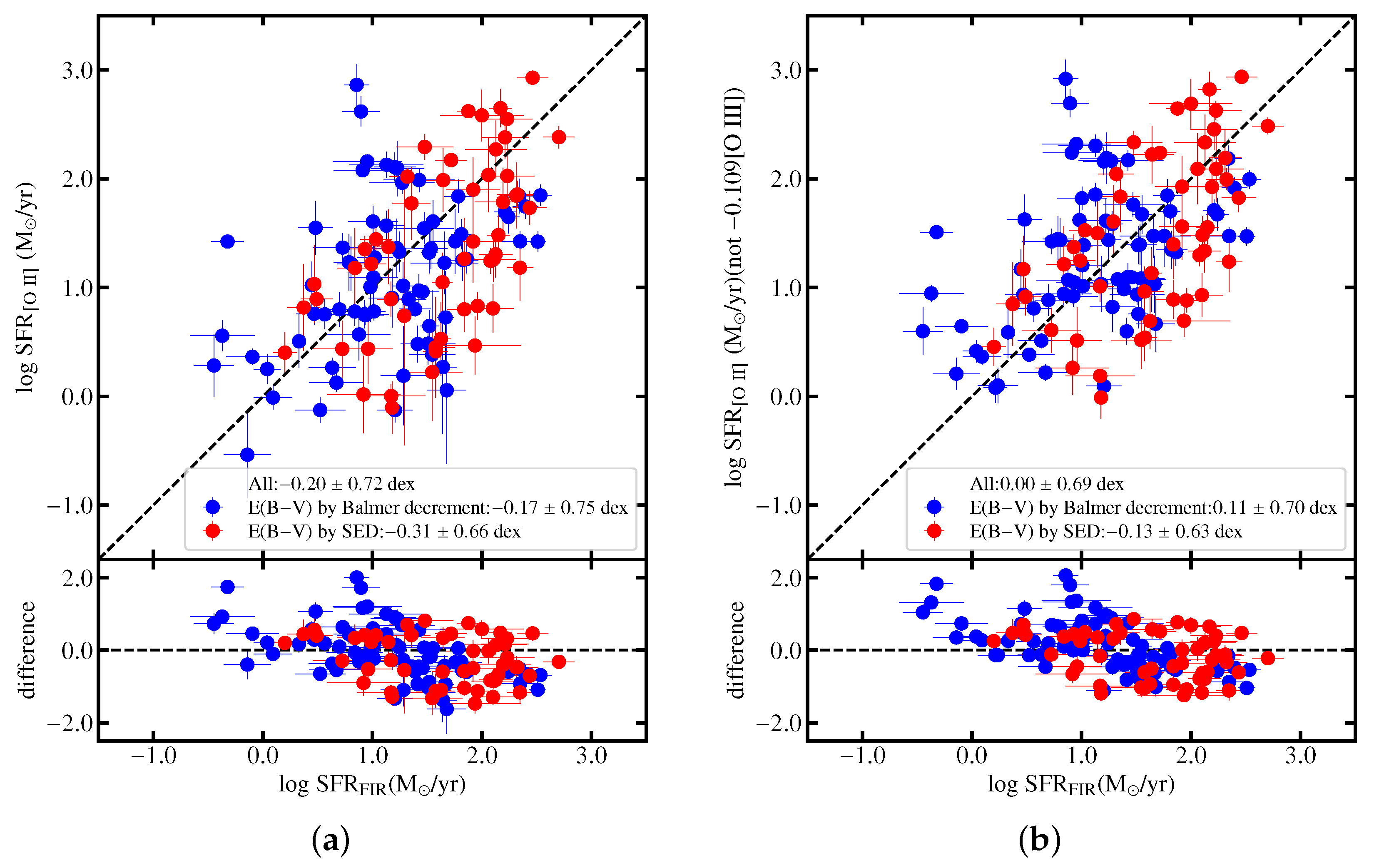
- We calculate [O ii] SFRs using the metallicity-dependent calibration of Zhuang and Ho [4]. We subtract the AGN NLR contribution to [O ii], estimated as . Extinction is corrected using the Balmer decrement when reliable narrow H and H measurements are available. Otherwise, we use the extinction obtained from SED fitting. The gas metallicity is estimated from the stellar mass–metallicity relation.
- 3.
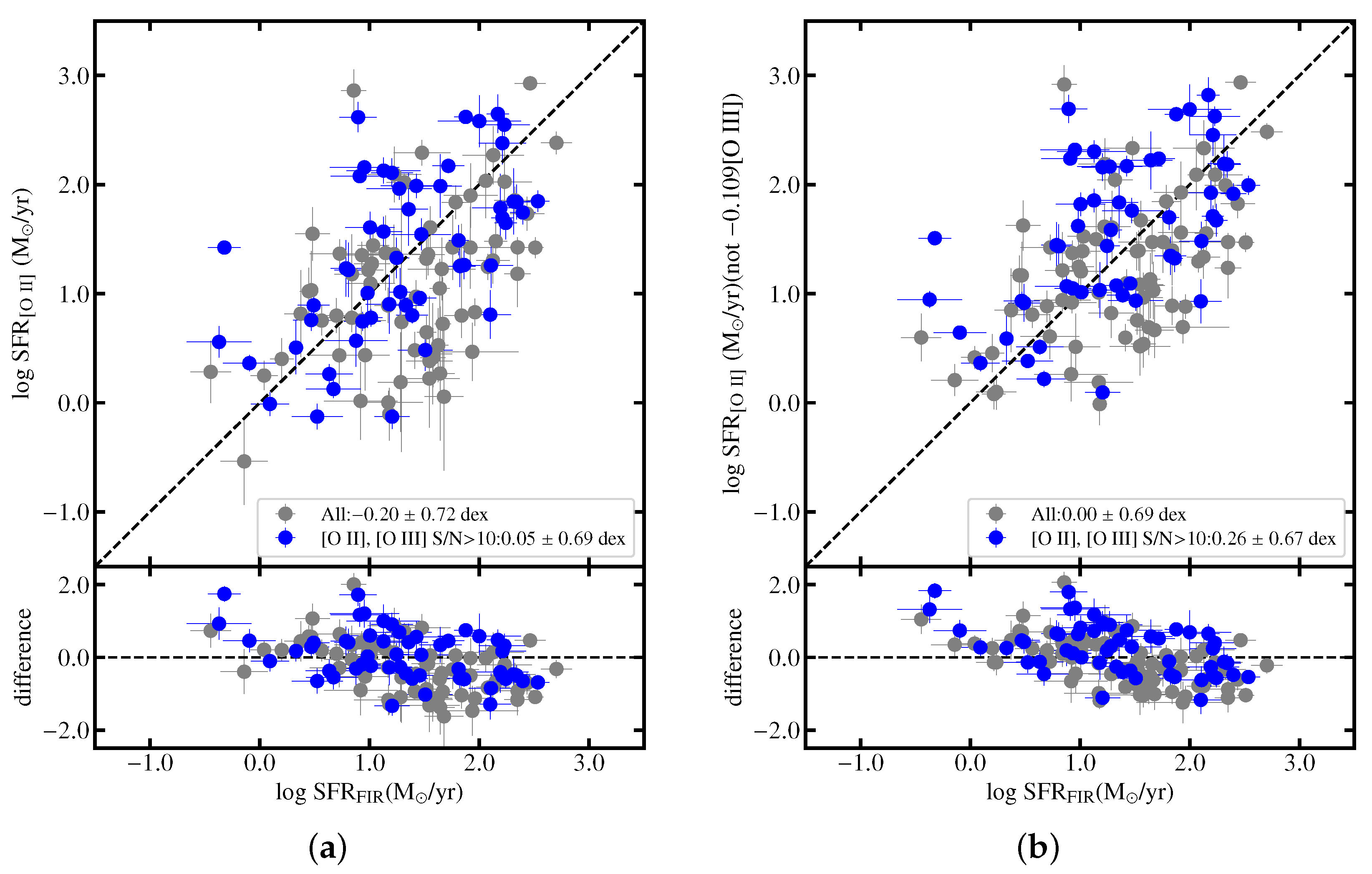
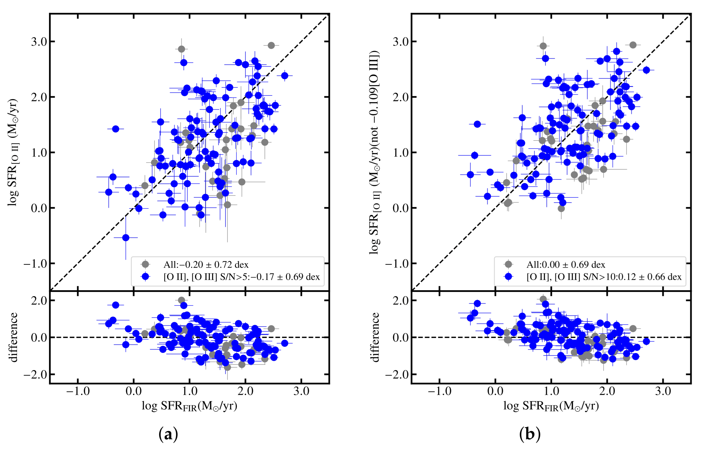
- After subtracting the contribution, [O ii] SFRs are mainly lower than FIR SFRs. The median offset is dex for the full sample and dex for sources with [O ii] and [O iii]. This suggests that the correction may oversubtract the star formation-related [O ii] luminosity for some quasars, although the large scatter indicates substantial object-to-object variation.
- 4.
- If the AGN NLR subtraction is not applied, the median offset becomes dex for the full sample and dex for the subsample. For the more strict subsample, the corrected [O ii] SFRs are comparable to FIR SFRs, with a median offset of dex, while the uncorrected [O ii] SFRs are higher by dex. These results show that the AGN contribution to [O ii] is non-negligible and should be considered when using [O ii] as an SFR tracer of quasar host galaxies.
- 5.
- The extinction correction is an important source of systematic uncertainty. Sources corrected using the SED extinction tend to have lower [O ii] SFRs than sources corrected using the Balmer decrement. This indicates that the uncertainty of the narrow-line gas extinction can contribute significantly to the scatter between [O ii] and FIR SFRs.
- 6.
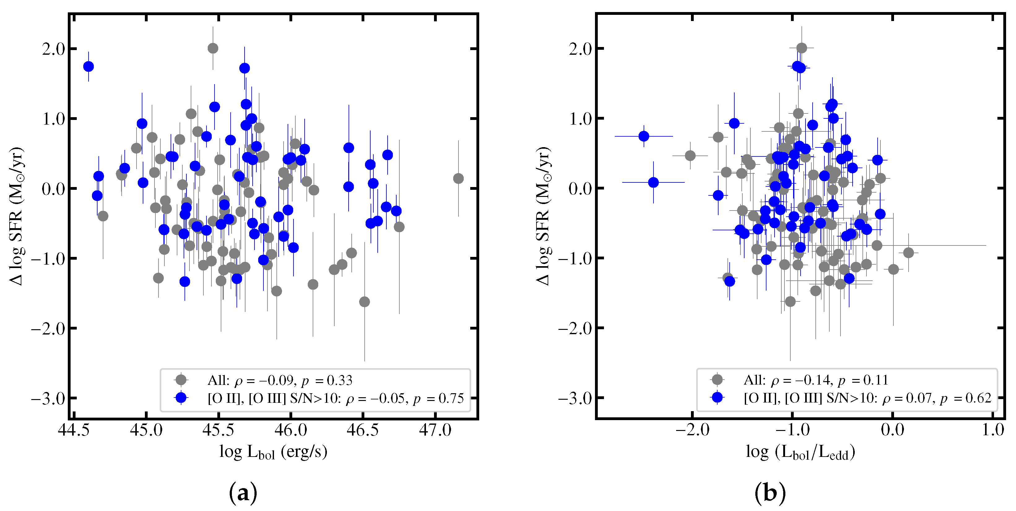
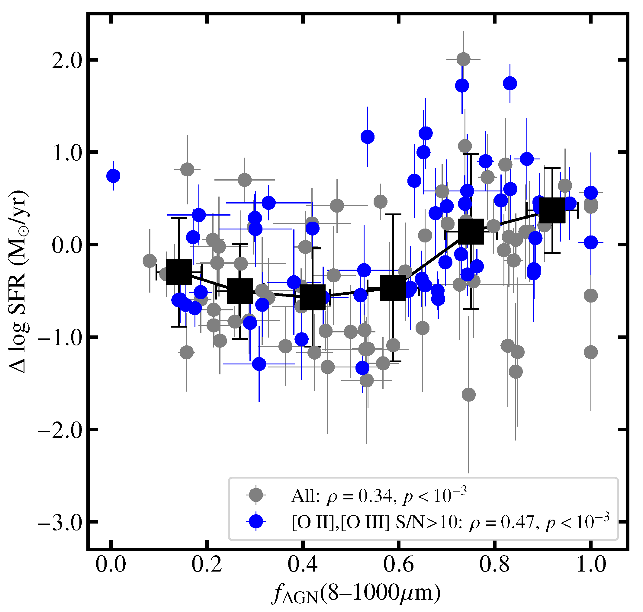
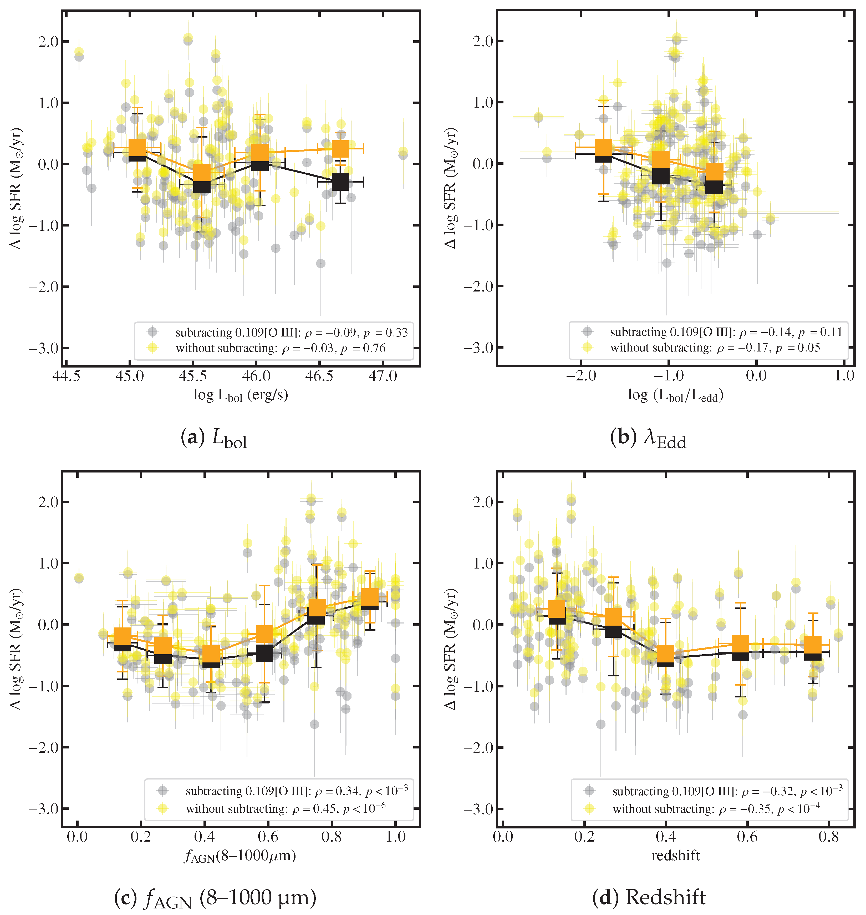
- We find no statistically significant correlation between the SFR offset and bolometric luminosity or Eddington ratio. However, the SFR offset shows a weak positive correlation with the fractional AGN contribution to the total infrared luminosity, (8–1000 µm), with and for the full sample. The correlation is stronger for the high S/N subsample. This trend may reflect the combined effects of AGN contamination, SED decomposition component degeneracy, and the relative contributions of AGN-heated dust and cold dust.
- 7.
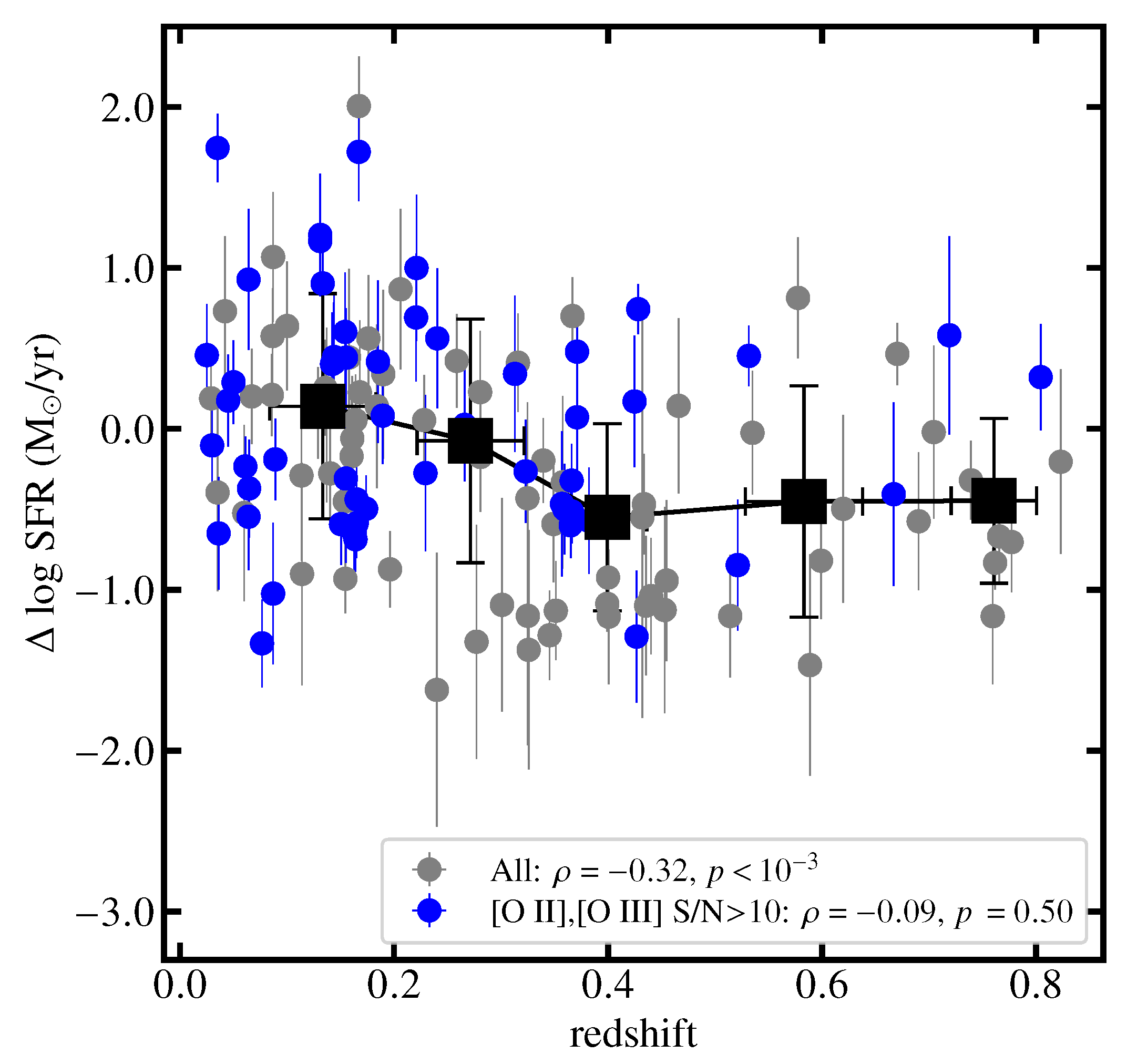
- The SFR offset shows a weak negative correlation with redshift for the full sample, with and . The [O ii] SFRs are close to the FIR SFRs at , but tend to be lower than the FIR SFRs at –0.5. This redshift dependence may partly arise from methodological effects, including the lack of H coverage at higher redshift, increased reliance on SED extinction corrections, aperture effects, FIR selection bias, and uncertainties in the AGN NLR correction.
Author Contributions
Funding
Data Availability Statement
Acknowledgments
Conflicts of Interest
Abbreviations
| AGN | Active galactic nucleus |
| BC | Balmer continuum |
| DBSP | Double Spectrograph |
| FIR | Far-infrared |
| FWHM | Full width at half maximum |
| HCT | Himalayan Chandra Telescope |
| IRSA | NASA/IPAC Infrared Science Archive |
| JCMT | James Clerk Maxwell Telescope |
| LJT | Lijiang 2.4 m Telescope |
| NED | NASA/IPAC Extragalactic Database |
| NLR | Narrow-line region |
| PACS | Photodetector Array Camera and Spectrometer |
| PCA | Principal component analysis |
| PG | Palomar-Green |
| SDSS | Sloan Digital Sky Survey |
| SED | Spectral energy distribution |
| SFR | Star formation rate |
| S/N | Signal-to-noise ratio |
| SPIRE | Spectral and Photometric Imaging Receiver |
| XLT | Xinglong 2.16 m Telescope |
Appendix A. Emission-Line and Star Formation Rate Measurements

| No. | Name | z | ||||
|---|---|---|---|---|---|---|
| () | () | () | () | |||
| 1 | J001115.69+011459.23 | 0.580 | 41.60 ± 0.10 | 41.28 ± 0.36 | – | 41.51 ± 0.08 |
| 2 | J002421.84+002508.49 | 0.599 | 41.39 ± 0.10 | 41.50 ± 0.08 | – | 41.81 ± 0.05 |
| 3 | J005905.51+000651.67 | 0.719 | 42.46 ± 0.02 | 43.11 ± 0.02 | – | 42.50 ± 0.02 |
| 4 | J011430.24+000420.94 | 0.455 | 41.05 ± 0.09 | 40.26 ± 1.40 | – | 39.89 ± 0.84 |
| 5 | J011536.92-000011.01 | 0.532 | 41.67 ± 0.03 | 42.21 ± 0.02 | – | 41.51 ± 0.06 |
| 6 | J013354.30+011034.00 | 0.704 | 41.78 ± 0.05 | 41.86 ± 0.11 | – | 41.48 ± 0.35 |
| 7 | J014003.99-002541.77 | 0.770 | 42.08 ± 0.03 | 41.89 ± 0.27 | – | 41.46 ± 0.25 |
| 8 | J015243.15+002039.65 | 0.578 | 41.78 ± 0.07 | 42.14 ± 0.06 | – | 41.15 ± 0.26 |
| 9 | J015950.25+002340.82 | 0.163 | 41.35 ± 0.02 | 42.26 ± 0.01 | 42.54 ± 0.01 | 41.59 ± 0.02 |
| 10 | J021859.87+002855.80 | 0.351 | 41.36 ± 0.06 | 41.55 ± 0.04 | 42.36 ± 0.03 | 41.87 ± 0.03 |
| 11 | J022430.61-000038.91 | 0.431 | 41.44 ± 0.03 | 41.42 ± 0.20 | – | 41.78 ± 0.07 |
| 12 | J090026.51+204158.70 | 0.706 | 41.96 ± 0.09 | 42.16 ± 1.65 | – | – |
| 13 | J090158.88+002313.87 | 0.196 | 41.23 ± 0.02 | 41.74 ± 0.04 | 41.76 ± 0.01 | 41.06 ± 0.03 |
| 14 | J090933.49+425346.51 | 0.670 | 42.65 ± 0.01 | 42.25 ± 0.13 | – | 41.62 ± 0.22 |
| 15 | J092159.40+450912.38 | 0.235 | 41.88 ± 0.01 | 41.20 ± 0.20 | 42.30 ± 0.02 | 41.55 ± 0.01 |
| 16 | J092554.72+195405.13 | 0.192 | 40.76 ± 0.23 | 42.09 ± 0.01 | 42.26 ± 0.03 | 41.84 ± 0.03 |
| 17 | J092635.12+072446.43 | 0.189 | 41.44 ± 0.01 | 42.03 ± 0.01 | 41.70 ± 0.02 | 40.91 ± 0.04 |
| 18 | J094652.58+131953.83 | 0.133 | 42.12 ± 0.01 | 42.44 ± 0.04 | 42.83 ± 0.01 | 42.01 ± 0.03 |
| 19 | J094745.14+072520.58 | 0.086 | 40.96 ± 0.02 | 41.56 ± 0.05 | 41.66 ± 0.01 | 41.02 ± 0.02 |
| 20 | J095017.06+215022.41 | 0.455 | 40.91 ± 0.14 | 41.91 ± 0.02 | 42.61 ± 0.01 | 41.77 ± 0.03 |
| 21 | J095240.17+515249.91 | 0.554 | 41.24 ± 0.13 | 42.25 ± 0.02 | – | 40.70 ± 0.58 |
| 22 | J095819.87+022903.51 | 0.345 | 40.80 ± 0.11 | 41.14 ± 0.10 | 41.49 ± 0.10 | 40.75 ± 0.10 |
| 23 | J100043.14+020637.25 | 0.360 | 41.20 ± 0.04 | 41.38 ± 0.15 | 41.90 ± 0.03 | 40.70 ± 0.08 |
| 24 | J100232.13+023537.33 | 0.658 | 41.60 ± 0.06 | 42.22 ± 0.05 | – | 41.89 ± 0.12 |
| 25 | J100420.13+051300.48 | 0.160 | 41.10 ± 0.05 | 41.81 ± 0.01 | 42.80 ± 0.01 | 42.05 ± 0.01 |
| 26 | J103651.94+575950.96 | 0.500 | 41.54 ± 0.06 | 41.65 ± 0.23 | – | 41.56 ± 0.12 |
| 27 | J104009.33+560343.28 | 0.393 | 41.44 ± 0.05 | 42.07 ± 0.03 | 42.56 ± 0.04 | 41.88 ± 0.05 |
| 28 | J104505.39+561118.34 | 0.428 | 42.36 ± 0.01 | 42.43 ± 0.04 | – | 41.87 ± 0.02 |
| 29 | J104739.49+563507.19 | 0.303 | 40.98 ± 0.08 | 41.18 ± 0.18 | 41.58 ± 0.11 | 40.96 ± 0.08 |
| 30 | J105106.12+591625.24 | 0.767 | 42.08 ± 0.09 | 42.45 ± 0.15 | – | – |
| 31 | J105143.89+335926.71 | 0.167 | 41.33 ± 0.04 | 42.06 ± 0.10 | 42.45 ± 0.01 | 41.23 ± 0.04 |
| 32 | J105151.44-005117.66 | 0.359 | 42.46 ± 0.02 | 43.37 ± 0.01 | 43.02 ± 0.01 | 42.31 ± 0.02 |
| 33 | J105705.41+580437.46 | 0.140 | 40.62 ± 0.05 | 41.35 ± 0.02 | 41.48 ± 0.02 | 40.60 ± 0.13 |
| 34 | J105959.93+574848.17 | 0.453 | 41.36 ± 0.06 | 42.38 ± 0.04 | – | 41.72 ± 0.04 |
| 35 | J110036.64+564134.89 | 0.834 | 41.58 ± 0.12 | – | – | – |
| 36 | J111706.40+441333.30 | 0.144 | 41.41 ± 0.04 | 42.25 ± 0.03 | 42.44 ± 0.01 | 41.65 ± 0.04 |
| 37 | J111830.29+402554.02 | 0.154 | 41.13 ± 0.06 | 41.63 ± 0.09 | 42.84 ± 0.01 | 42.17 ± 0.02 |
| 38 | J112019.62+130320.10 | 0.314 | 41.28 ± 0.04 | 41.54 ± 0.23 | 42.34 ± 0.01 | 41.13 ± 0.34 |
| 39 | J112048.99+133821.91 | 0.513 | 41.52 ± 0.05 | 41.83 ± 0.07 | – | 41.38 ± 0.06 |
| 40 | J112759.26+360207.00 | 0.667 | 41.84 ± 0.03 | 42.55 ± 0.03 | – | 41.45 ± 0.11 |
| 41 | J114121.76+014803.58 | 0.382 | 41.62 ± 0.04 | 42.09 ± 0.03 | 42.46 ± 0.02 | 41.73 ± 0.03 |
| 42 | J114933.88+222227.07 | 0.554 | 41.32 ± 0.09 | 41.27 ± 0.35 | – | 41.30 ± 0.11 |
| 43 | J115253.68+000131.90 | 0.823 | 41.91 ± 0.07 | 42.35 ± 0.07 | – | 41.51 ± 0.50 |
| 44 | J120226.76-012915.28 | 0.150 | 41.25 ± 0.02 | 41.36 ± 0.01 | 42.02 ± 0.01 | 41.10 ± 0.03 |
| 45 | J120312.14+015321.30 | 0.296 | 41.02 ± 0.04 | 40.80 ± 0.25 | 41.67 ± 0.02 | 41.54 ± 0.07 |
| 46 | J120442.11+275411.80 | 0.165 | 41.69 ± 0.01 | 42.32 ± 0.01 | 42.22 ± 0.01 | 41.59 ± 0.01 |
| 47 | J120734.63+150643.69 | 0.750 | 41.74 ± 0.08 | 42.56 ± 0.18 | – | 42.54 ± 0.12 |
| 48 | J121037.81+053805.88 | 0.436 | 41.09 ± 0.11 | 41.75 ± 0.08 | – | 41.44 ± 0.12 |
| 49 | J121728.37+065110.00 | 0.589 | 41.56 ± 0.09 | 42.19 ± 0.08 | – | 41.55 ± 0.15 |
| 50 | J121836.71+155908.43 | 0.766 | 42.01 ± 0.05 | 42.33 ± 0.10 | – | 42.45 ± 0.07 |
| 51 | J121906.57+160243.06 | 0.761 | 42.11 ± 0.03 | 41.55 ± 0.56 | – | 41.50 ± 0.34 |
| 52 | J121945.03+082117.95 | 0.228 | 41.18 ± 0.02 | 40.86 ± 0.10 | 42.05 ± 0.01 | 41.07 ± 0.03 |
| 53 | J121946.54+145259.37 | 0.401 | 41.38 ± 0.05 | 41.90 ± 0.05 | 41.14 ± 0.64 | 40.94 ± 0.15 |
| 54 | J122011.88+020342.21 | 0.240 | 41.95 ± 0.02 | 42.79 ± 0.01 | 42.89 ± 0.01 | 42.04 ± 0.02 |
| 55 | J122026.72+062748.20 | 0.349 | 40.67 ± 0.12 | 41.27 ± 0.14 | 40.82 ± 0.32 | 40.44 ± 0.16 |
| 56 | J122102.50+155447.04 | 0.229 | 41.17 ± 0.04 | 41.81 ± 0.01 | 42.08 ± 0.03 | 41.30 ± 0.05 |
| 57 | J122102.95-000733.74 | 0.366 | 41.94 ± 0.01 | 41.64 ± 0.03 | 42.69 ± 0.02 | 41.96 ± 0.01 |
| 58 | J122106.50+114625.46 | 0.340 | 41.40 ± 0.03 | 41.80 ± 0.06 | 42.10 ± 0.02 | 41.31 ± 0.03 |
| 59 | J122307.37-002124.73 | 0.804 | 42.09 ± 0.03 | 42.68 ± 0.02 | – | 41.40 ± 0.34 |
| 60 | J122312.17+095017.72 | 0.277 | 40.96 ± 0.08 | 41.80 ± 0.10 | 41.83 ± 0.11 | 41.40 ± 0.10 |
| 61 | J122317.80+092306.94 | 0.682 | 41.94 ± 0.10 | 41.86 ± 0.15 | – | 42.48 ± 0.04 |
| 62 | J122404.62+045637.94 | 0.358 | 41.80 ± 0.02 | 42.01 ± 0.11 | 42.44 ± 0.04 | 41.72 ± 0.06 |
| 63 | J122520.13+084450.76 | 0.535 | 41.94 ± 0.06 | 42.31 ± 0.05 | – | 42.02 ± 0.07 |
| 64 | J122526.21+141332.24 | 0.760 | 41.76 ± 0.09 | 41.94 ± 0.11 | – | 42.19 ± 0.07 |
| 65 | J122641.50+055906.81 | 0.290 | 41.11 ± 0.06 | 41.74 ± 0.16 | 41.78 ± 0.02 | 40.99 ± 0.07 |
| 66 | J122822.10+114606.83 | 0.365 | 41.71 ± 0.02 | 41.98 ± 0.01 | 42.24 ± 0.02 | 41.56 ± 0.02 |
| 67 | J122839.20+035749.29 | 0.608 | 41.35 ± 0.07 | 41.57 ± 0.36 | – | 40.94 ± 0.47 |
| 68 | J123436.54+123918.66 | 0.777 | 42.10 ± 0.02 | 42.56 ± 0.07 | – | 41.67 ± 0.19 |
| 69 | J123800.92+621336.09 | 0.440 | 41.15 ± 0.09 | 41.61 ± 0.03 | – | 41.65 ± 0.06 |
| 70 | J124511.26+335610.12 | 0.711 | – | 42.41 ± 0.02 | – | 42.36 ± 0.05 |
| 71 | J125257.36+331555.81 | 0.367 | 41.50 ± 0.03 | 41.63 ± 0.06 | 41.84 ± 0.11 | 41.09 ± 0.09 |
| 72 | J125317.57+310550.64 | 0.782 | 42.29 ± 0.05 | 42.90 ± 0.08 | – | 42.41 ± 0.14 |
| 73 | J125553.05+272405.23 | 0.316 | 41.04 ± 0.07 | 41.65 ± 0.03 | 41.65 ± 0.07 | 40.87 ± 0.12 |
| 74 | J125703.80+250457.56 | 0.821 | 41.65 ± 0.09 | – | – | – |
| 75 | J125711.97+274216.45 | 0.793 | 41.76 ± 0.04 | 41.91 ± 0.36 | – | 41.45 ± 0.39 |
| 76 | J125757.23+322929.29 | 0.806 | 41.39 ± 0.22 | 42.44 ± 0.03 | – | 41.72 ± 0.22 |
| 77 | J130622.96+225752.95 | 0.758 | 41.70 ± 0.06 | 40.94 ± 1.14 | – | 41.30 ± 0.32 |
| 78 | J130947.00+081948.23 | 0.154 | 41.71 ± 0.03 | 42.57 ± 0.03 | 42.66 ± 0.01 | 41.84 ± 0.02 |
| 79 | J131247.97+250756.71 | 0.425 | 42.11 ± 0.02 | 42.64 ± 0.01 | – | 41.87 ± 0.02 |
| 80 | J131312.13+284730.01 | 0.259 | 40.83 ± 0.07 | 40.85 ± 0.12 | – | 40.31 ± 0.15 |
| 81 | J131531.66+265414.73 | 0.620 | 41.59 ± 0.08 | 42.28 ± 0.11 | – | 41.50 ± 0.17 |
| 82 | J132919.84+250626.45 | 0.781 | 41.39 ± 0.13 | 41.58 ± 0.25 | – | – |
| 83 | J133005.71+254243.77 | 0.598 | – | 42.34 ± 0.03 | – | 41.56 ± 0.13 |
| 84 | J133442.29+320939.60 | 0.649 | 41.24 ± 0.20 | 41.51 ± 0.22 | – | 42.28 ± 0.06 |
| 85 | J134356.74+253847.69 | 0.086 | 40.63 ± 0.05 | 41.49 ± 0.03 | 41.69 ± 0.01 | 40.74 ± 0.03 |
| 86 | J135632.80+210352.35 | 0.301 | 41.58 ± 0.06 | 42.57 ± 0.01 | 42.43 ± 0.03 | 41.79 ± 0.03 |
| 87 | J140621.89+222346.54 | 0.098 | 40.29 ± 0.09 | – | 42.51 ± 0.00 | 41.93 ± 0.00 |
| 88 | J140655.66+015712.88 | 0.427 | 41.40 ± 0.04 | 41.93 ± 0.02 | – | 41.88 ± 0.05 |
| 89 | J140700.40+282714.65 | 0.077 | 41.10 ± 0.02 | 41.75 ± 0.01 | 41.84 ± 0.01 | 41.26 ± 0.02 |
| 90 | J141637.45+003352.28 | 0.434 | 41.83 ± 0.02 | 42.55 ± 0.04 | – | 41.74 ± 0.03 |
| 91 | J141644.62+190541.92 | 0.365 | 41.27 ± 0.04 | 40.15 ± 1.17 | 41.97 ± 0.03 | 41.31 ± 0.14 |
| 92 | J141700.83+445606.39 | 0.113 | 40.45 ± 0.07 | 41.25 ± 0.04 | 42.25 ± 0.01 | – |
| 93 | J142052.44+525622.42 | 0.677 | 41.68 ± 0.08 | 42.50 ± 0.02 | – | 42.13 ± 0.04 |
| 94 | J142648.78+005323.24 | 0.220 | 41.50 ± 0.01 | 41.92 ± 0.16 | 42.20 ± 0.01 | 41.21 ± 0.04 |
| 95 | J142710.94+013023.22 | 0.704 | 42.30 ± 0.04 | 41.86 ± 0.26 | – | 41.91 ± 0.27 |
| 96 | J142753.79+345248.35 | 0.514 | 41.26 ± 0.12 | 41.75 ± 0.04 | – | 42.18 ± 0.03 |
| 97 | J142918.15+592106.65 | 0.739 | 42.24 ± 0.02 | 42.86 ± 0.08 | – | 42.16 ± 0.06 |
| 98 | J142943.07+474726.23 | 0.221 | 41.53 ± 0.02 | 42.51 ± 0.01 | 42.91 ± 0.00 | 41.95 ± 0.01 |
| 99 | J143624.81-002905.36 | 0.325 | 40.93 ± 0.10 | 41.98 ± 0.01 | 42.70 ± 0.01 | 41.73 ± 0.03 |
| 100 | J144231.82+014353.43 | 0.280 | 40.79 ± 0.08 | 40.98 ± 0.12 | 41.71 ± 0.04 | 40.82 ± 0.14 |
| 101 | J145001.69+022006.75 | 0.520 | 41.75 ± 0.04 | – | – | 41.81 ± 0.08 |
| 102 | J145108.76+270926.92 | 0.064 | 41.02 ± 0.02 | 41.77 ± 0.01 | 42.50 ± 0.01 | 41.85 ± 0.01 |
| 103 | J145538.73+002238.06 | 0.434 | 40.83 ± 0.16 | 41.61 ± 0.05 | – | 41.19 ± 0.09 |
| 104 | J152114.26+222743.87 | 0.136 | 40.87 ± 0.05 | 41.62 ± 0.01 | 42.72 ± 0.01 | 41.78 ± 0.02 |
| 105 | J154530.24+484608.98 | 0.399 | 41.68 ± 0.05 | 41.89 ± 0.03 | 43.48 ± 0.00 | 42.75 ± 0.01 |
| 106 | J155444.58+082221.48 | 0.119 | 40.42 ± 0.10 | 41.56 ± 0.01 | 42.70 ± 0.00 | 42.00 ± 0.01 |
| 107 | J161413.20+260416.21 | 0.131 | 42.24 ± 0.01 | 43.00 ± 0.02 | 42.83 ± 0.00 | 42.01 ± 0.01 |
| 108 | J163352.34+402115.66 | 0.782 | 41.79 ± 0.05 | 42.12 ± 0.18 | – | 41.97 ± 0.12 |
| 109 | J163915.81+412833.70 | 0.690 | 41.66 ± 0.13 | 42.26 ± 0.04 | – | 41.53 ± 0.15 |
| 110 | J171033.22+584456.86 | 0.281 | 41.01 ± 0.05 | 41.25 ± 0.04 | 41.98 ± 0.01 | 41.09 ± 0.03 |
| 111 | J171352.43+584201.25 | 0.521 | 42.03 ± 0.03 | 42.74 ± 0.02 | – | 41.63 ± 0.07 |
| 112 | J220759.39+001722.62 | 0.368 | 40.84 ± 0.08 | 40.71 ± 0.20 | 42.75 ± 0.00 | 42.08 ± 0.01 |
| 113 | J223607.68+134355.32 | 0.326 | 41.49 ± 0.05 | 42.58 ± 0.01 | 43.32 ± 0.00 | 42.62 ± 0.07 |
| 114 | J233741.32+001743.77 | 0.762 | 41.66 ± 0.06 | 41.88 ± 0.08 | – | 41.70 ± 0.05 |
| 115 | J235156.13-010913.34 | 0.174 | 41.73 ± 0.01 | 42.23 ± 0.01 | 42.20 ± 0.00 | 41.57 ± 0.01 |
| No. | Name | z | ||||
|---|---|---|---|---|---|---|
| () | () | () | () | |||
| 1 | PG0157+001 | 0.164 | 41.41 ± 0.02 | 42.26 ± 0.01 | 42.55 ± 0.00 | 41.60 ± 0.02 |
| 2 | PG0921+525 | 0.035 | 41.21 ± 0.00 | 41.80 ± 0.01 | 41.69 ± 0.01 | 40.80 ± 0.01 |
| 3 | PG0923+201 | 0.190 | 41.18 ± 0.11 | 41.32 ± 0.05 | 40.99 ± 0.35 | 41.26 ± 0.11 |
| 4 | PG0934+013 | 0.050 | 40.56 ± 0.02 | 41.44 ± 0.01 | 41.78 ± 0.00 | 40.86 ± 0.02 |
| 5 | PG0947+396 | 0.206 | 41.32 ± 0.07 | 42.08 ± 0.01 | 42.36 ± 0.01 | 41.33 ± 0.04 |
| 6 | PG1001+054 | 0.161 | 41.11 ± 0.05 | 41.81 ± 0.01 | 42.81 ± 0.00 | 42.06 ± 0.01 |
| 7 | PG1004+130 | 0.240 | 41.53 ± 0.12 | 42.43 ± 0.01 | 42.50 ± 0.01 | 41.95 ± 0.03 |
| 8 | PG1022+519 | 0.045 | 40.34 ± 0.03 | 40.89 ± 0.01 | 41.56 ± 0.05 | 40.70 ± 0.02 |
| 9 | PG1048+342 | 0.167 | 41.11 ± 0.04 | 41.96 ± 0.01 | 42.55 ± 0.00 | 41.33 ± 0.02 |
| 10 | PG1049-005 | 0.357 | 42.45 ± 0.02 | 43.36 ± 0.01 | 41.98 ± 0.11 | 42.31 ± 0.02 |
| 11 | PG1114+445 | 0.144 | 41.41 ± 0.04 | 42.25 ± 0.04 | 42.44 ± 0.01 | 41.64 ± 0.05 |
| 12 | PG1115+407 | 0.154 | 41.17 ± 0.06 | 41.80 ± 0.01 | 42.84 ± 0.01 | 42.06 ± 0.02 |
| 13 | PG1121+422 | 0.234 | 41.36 ± 0.05 | 41.90 ± 0.14 | 43.11 ± 0.19 | 42.37 ± 0.07 |
| 14 | PG1151+117 | 0.176 | 41.25 ± 0.06 | 41.91 ± 0.08 | 42.02 ± 0.04 | 41.35 ± 0.17 |
| 15 | PG1202+281 | 0.165 | 41.69 ± 0.01 | 42.32 ± 0.01 | 42.22 ± 0.01 | 41.59 ± 0.01 |
| 16 | PG1229+204 | 0.064 | 40.81 ± 0.02 | 41.19 ± 0.02 | 41.81 ± 0.01 | 41.18 ± 0.01 |
| 17 | PG1244+026 | 0.048 | 40.50 ± 0.03 | 40.40 ± 0.44 | 41.72 ± 0.01 | 41.26 ± 0.04 |
| 18 | PG1259+593 | 0.472 | – | – | – | – |
| 19 | PG1309+355 | 0.184 | 41.44 ± 0.07 | 42.38 ± 0.02 | 42.63 ± 0.01 | 41.79 ± 0.04 |
| 20 | PG1341+258 | 0.087 | 40.73 ± 0.04 | 41.41 ± 0.05 | 41.69 ± 0.01 | 40.66 ± 0.05 |
| 21 | PG1415+451 | 0.114 | 40.41 ± 0.08 | 41.25 ± 0.06 | 42.25 ± 0.01 | – |
| 22 | PG1425+267 | 0.366 | 42.16 ± 0.02 | 42.87 ± 0.02 | 42.67 ± 0.01 | 42.01 ± 0.02 |
| 23 | PG1427+480 | 0.221 | 41.45 ± 0.03 | 42.44 ± 0.01 | 42.95 ± 0.00 | 41.92 ± 0.02 |
| 24 | PG1444+407 | 0.267 | 40.98 ± 0.33 | 42.17 ± 0.01 | 43.08 ± 0.01 | 42.42 ± 0.02 |
| 25 | PG1512+370 | 0.371 | 42.16 ± 0.03 | 42.90 ± 0.02 | 42.77 ± 0.01 | 42.08 ± 0.02 |
| 26 | PG1534+580 | 0.030 | 40.63 ± 0.01 | 41.60 ± 0.01 | 41.36 ± 0.01 | 40.61 ± 0.01 |
| 27 | PG1543+489 | 0.400 | 41.68 ± 0.05 | 41.89 ± 0.03 | 43.48 ± 0.00 | 42.75 ± 0.01 |
| 28 | PG1552+085 | 0.119 | 40.43 ± 0.12 | 41.56 ± 0.01 | 42.70 ± 0.01 | 42.01 ± 0.01 |
| 29 | PG1612+261 | 0.131 | 42.24 ± 0.01 | 43.00 ± 0.03 | 42.83 ± 0.00 | 42.01 ± 0.01 |
| 30 | PG1704+608 | 0.371 | 42.53 ± 0.02 | 43.36 ± 0.01 | 45.80 ± 0.22 | 42.47 ± 0.01 |
| 31 | PG2233+134 | 0.325 | 41.51 ± 0.07 | 42.58 ± 0.01 | 43.32 ± 0.00 | 42.62 ± 0.05 |
| No. | Name | z | Instrument | ||||
|---|---|---|---|---|---|---|---|
| () | () | () | () | ||||
| 1 | PG0003+158 | 0.450 | 42.33 ± 0.07 | 43.60 ± 0.01 | – | 43.00 ± 0.02 | LJT |
| 2 | PG0003+199 | 0.025 | 40.82 ± 0.03 | 41.72 ± 0.00 | 42.29 ± 0.00 | 41.53 ± 0.01 | HCT |
| 3 | PG0007+106 | 0.089 | 41.83 ± 0.01 | 42.57 ± 0.00 | 42.11 ± 0.01 | 41.53 ± 0.01 | HCT |
| 4 | PG0026+129 | 0.142 | 41.57 ± 0.02 | 41.36 ± 0.04 | 42.05 ± 0.02 | – | XLT |
| 5 | PG0043+039 | 0.384 | 41.83 ± 0.08 | 41.87 ± 0.14 | – | – | XLT |
| 6 | PG0049+171 | 0.064 | 41.07 ± 0.04 | 42.11 ± 0.01 | 42.19 ± 0.00 | 41.38 ± 0.01 | HCT |
| 7 | PG0050+124 | 0.061 | 40.28 ± 0.20 | 41.24 ± 0.05 | 42.61 ± 0.00 | 41.71 ± 0.01 | LJT |
| 8 | PG0052+251 | 0.155 | 41.98 ± 0.02 | 42.88 ± 0.01 | 42.72 ± 0.01 | 41.96 ± 0.02 | LJT |
| 9 | PG0804+761 | 0.100 | 41.68 ± 0.05 | 41.95 ± 0.04 | 43.00 ± 0.01 | 42.29 ± 0.01 | LJT |
| 10 | PG0838+770 | 0.131 | 40.56 ± 0.20 | 41.35 ± 0.14 | 42.08 ± 0.01 | 41.34 ± 0.06 | LJT |
| 11 | PG0844+349 | 0.064 | 40.87 ± 0.15 | 41.69 ± 0.01 | 42.28 ± 0.00 | 41.47 ± 0.02 | LJT |
| 12 | PG0923+129 | 0.029 | 40.60 ± 0.05 | 40.97 ± 0.06 | 41.87 ± 0.01 | 41.02 ± 0.02 | LJT |
| 13 | PG0953+414 | 0.239 | – | 42.19 ± 0.03 | 43.32 ± 0.11 | – | XLT |
| 14 | PG1011-040 | 0.058 | 40.09 ± 0.12 | 41.16 ± 0.01 | 41.30 ± 0.01 | 40.84 ± 0.02 | HCT |
| 15 | PG1012+008 | 0.185 | 41.78 ± 0.03 | 42.16 ± 0.02 | 42.36 ± 0.02 | 41.92 ± 0.03 | HCT |
| 16 | PG1048-090 | 0.344 | 42.14 ± 0.16 | 43.33 ± 0.01 | – | 42.59 ± 0.03 | XLT |
| 17 | PG1100+772 | 0.313 | 42.52 ± 0.02 | 43.31 ± 0.02 | 42.41 ± 0.28 | 42.39 ± 0.03 | XLT |
| 18 | PG1103-006 | 0.425 | 42.08 ± 0.13 | 42.65 ± 0.16 | – | 42.30 ± 0.16 | XLT |
| 19 | PG1116+215 | 0.177 | 41.46 ± 0.23 | 40.92 ± 0.82 | 43.15 ± 0.01 | 42.54 ± 0.02 | XLT |
| 20 | PG1119+120 | 0.049 | – | – | 42.10 ± 0.01 | 41.08 ± 0.05 | LJT |
| 21 | PG1126-041 | 0.060 | 40.83 ± 0.06 | 41.20 ± 0.06 | 41.71 ± 0.01 | 41.59 ± 0.01 | HCT |
| 22 | PG1149-110 | 0.049 | 40.77 ± 0.02 | 39.64 ± 5.52 | 39.40 ± 0.52 | 39.59 ± 0.30 | HCT |
| 23 | PG1211+143 | 0.085 | 41.35 ± 0.03 | – | 43.01 ± 0.00 | – | LJT |
| 24 | PG1216+069 | 0.334 | 42.21 ± 0.14 | 42.96 ± 0.12 | 43.11 ± 0.15 | 42.38 ± 0.12 | XLT |
| 25 | PG1226+023 | 0.158 | 42.40 ± 0.09 | 41.38 ± 0.45 | 43.61 ± 0.01 | 43.11 ± 0.02 | XLT |
| 26 | PG1307+085 | 0.155 | 41.88 ± 0.03 | 42.75 ± 0.02 | 42.57 ± 0.01 | 42.00 ± 0.03 | XLT |
| 27 | PG1310-108 | 0.035 | 40.47 ± 0.05 | 41.61 ± 0.01 | 41.43 ± 0.01 | 40.66 ± 0.02 | LJT |
| 28 | PG1322+659 | 0.168 | 41.44 ± 0.07 | 42.10 ± 0.01 | 42.49 ± 0.01 | 40.84 ± 0.58 | XLT |
| 29 | PG1351+640 | 0.087 | 41.69 ± 0.04 | 42.59 ± 0.01 | 42.72 ± 0.00 | 42.10 ± 0.01 | HCT |
| 30 | PG1352+183 | 0.158 | 40.84 ± 0.14 | 40.94 ± 0.09 | – | – | XLT |
| 31 | PG1354+213 | 0.300 | 41.88 ± 0.07 | – | 42.62 ± 0.02 | 42.08 ± 0.07 | XLT |
| 32 | PG1402+261 | 0.164 | 41.65 ± 0.07 | 42.06 ± 0.02 | 42.97 ± 0.00 | 42.16 ± 0.03 | XLT |
| 33 | PG1411+442 | 0.089 | 41.18 ± 0.24 | 42.28 ± 0.01 | 42.70 ± 0.01 | 42.07 ± 0.03 | HCT |
| 34 | PG1416-129 | 0.129 | 41.60 ± 0.01 | 41.93 ± 0.06 | 41.95 ± 0.01 | 41.34 ± 0.03 | LJT |
| 35 | PG1426+015 | 0.086 | 41.14 ± 0.18 | 41.37 ± 0.21 | 41.82 ± 0.04 | 40.65 ± 0.45 | LJT |
| 36 | PG1440+356 | 0.077 | 41.08 ± 0.10 | 41.26 ± 0.27 | 42.61 ± 0.01 | 41.67 ± 0.03 | LJT |
| 37 | PG1448+273 | 0.065 | 41.35 ± 0.04 | 41.66 ± 0.19 | 41.65 ± 0.05 | 41.55 ± 0.04 | LJT |
| 38 | PG1501+106 | 0.036 | 41.09 ± 0.02 | 42.00 ± 0.00 | 41.82 ± 0.00 | 41.22 ± 0.01 | LJT |
| 39 | PG1519+226 | 0.137 | 40.66 ± 0.13 | 41.40 ± 0.02 | 42.58 ± 0.00 | 41.65 ± 0.04 | LJT |
| 40 | PG1535+547 | 0.038 | – | 40.86 ± 0.01 | 42.00 ± 0.00 | 41.23 ± 0.01 | LJT |
| 41 | PG1545+210 | 0.266 | 42.23 ± 0.04 | 43.20 ± 0.02 | 43.15 ± 0.01 | 42.52 ± 0.03 | LJT |
| 42 | PG1613+658 | 0.129 | 41.71 ± 0.03 | 42.24 ± 0.02 | 41.83 ± 0.03 | 40.57 ± 0.37 | LJT |
| 43 | PG1617+175 | 0.114 | 41.00 ± 0.07 | – | 42.24 ± 0.01 | 41.09 ± 0.09 | DBSP |
| 44 | PG1626+554 | 0.133 | 40.63 ± 0.15 | – | 42.37 ± 0.01 | 41.58 ± 0.07 | LJT |
| 45 | PG1700+518 | 0.282 | – | – | 43.65 ± 0.00 | – | LJT |
| 46 | PG2112+059 | 0.466 | 42.23 ± 0.05 | 42.63 ± 0.02 | – | 41.41 ± 0.39 | XLT |
| 47 | PG2130+099 | 0.061 | 41.02 ± 0.03 | 41.91 ± 0.01 | 42.75 ± 0.00 | 41.94 ± 0.01 | LJT |
| 48 | PG2209+184 | 0.070 | 40.98 ± 0.09 | 40.57 ± 0.63 | – | – | HCT |
| 49 | PG2214+139 | 0.067 | 41.15 ± 0.10 | 41.28 ± 0.02 | 41.89 ± 0.01 | – | HCT |
| 50 | PG2251+113 | 0.323 | 42.42 ± 0.03 | 43.32 ± 0.01 | 43.21 ± 0.01 | 42.65 ± 0.02 | XLT |
| 51 | PG2304+042 | 0.042 | 40.64 ± 0.05 | 41.59 ± 0.01 | 41.29 ± 0.03 | 40.51 ± 0.04 | HCT |
| 52 | PG2308+098 | 0.432 | 42.00 ± 0.10 | 43.08 ± 0.04 | – | 42.57 ± 0.03 | XLT |
| Sample ID | Name | z | ||||||
|---|---|---|---|---|---|---|---|---|
| () | () | () | () | () | ||||
| 1 | J001115.69+011459.23 | 0.580 | 2.34 ± 0.15 | 0.86 ± 0.04 | 43.20 ± 0.17 | 42.47 ± 0.42 | 2.10 ± 0.18 | 2.11 ± 0.17 |
| 2 | J002421.84+002508.49 | 0.599 | 2.12 ± 0.15 | 0.59 ± 0.05 | 42.50 ± 0.20 | 42.32 ± 0.15 | 1.30 ± 0.21 | 1.34 ± 0.20 |
| 3 | J005905.51+000651.67 | 0.719 | 2.00 ± 0.38 | 0.72 ± 0.11 | 43.80 ± 0.23 | 44.10 ± 0.17 | 2.58 ± 0.24 | 2.69 ± 0.23 |
| 4 | J011430.24+000420.94 | 0.455 | 1.43 ± 0.14 | 0.89 ± 0.02 | 42.72 ± 0.12 | 41.50 ± 1.42 | 1.60 ± 0.13 | 1.61 ± 0.12 |
| 5 | J011536.92-000011.01 | 0.532 | 1.72 ± 0.14 | 0.90 ± 0.00 | 43.35 ± 0.04 | 43.46 ± 0.02 | 2.17 ± 0.04 | 2.24 ± 0.04 |
| 6 | J013354.30+011034.00 | 0.704 | 1.92 ± 0.24 | 0.67 ± 0.12 | 43.04 ± 0.28 | 42.79 ± 0.28 | 1.90 ± 0.29 | 1.93 ± 0.28 |
| 7 | J014003.99-002541.77 | 0.770 | 2.40 ± 0.19 | 0.53 ± 0.09 | 43.07 ± 0.20 | 42.62 ± 0.39 | 1.95 ± 0.21 | 1.97 ± 0.20 |
| 8 | J015243.15+002039.65 | 0.578 | 1.48 ± 0.26 | 0.89 ± 0.02 | 43.45 ± 0.10 | 43.38 ± 0.09 | 2.29 ± 0.12 | 2.33 ± 0.10 |
| 9 | J015950.25+002340.82 | 0.163 | 2.40 ± 0.12 | 0.91 ± 0.04 | 43.04 ± 0.09 | 43.51 ± 0.06 | 1.74 ± 0.11 | 1.92 ± 0.09 |
| 10 | J021859.87+002855.80 | 0.351 | 1.96 ± 0.18 | 0.37 ± 0.03 | 42.06 ± 0.11 | 42.07 ± 0.08 | 0.83 ± 0.12 | 0.88 ± 0.11 |
| 11 | J022430.61-000038.91 | 0.431 | 1.41 ± 0.13 | 0.64 ± 0.11 | 42.63 ± 0.23 | 42.31 ± 0.35 | 1.34 ± 0.24 | 1.37 ± 0.23 |
| 12 | J090026.51+204158.70 | 0.706 | 2.35 ± 0.06 | 0.20 ± 0.01 | 42.34 ± 0.10 | 42.45 ± 1.67 | 1.16 ± 0.39 | 1.23 ± 0.10 |
| 13 | J090158.88+002313.87 | 0.196 | 1.52 ± 0.09 | 0.42 ± 0.06 | 42.01 ± 0.13 | 42.32 ± 0.13 | 0.65 ± 0.15 | 0.76 ± 0.13 |
| 14 | J090933.49+425346.51 | 0.670 | 2.46 ± 0.14 | 0.75 ± 0.02 | 44.05 ± 0.05 | 43.28 ± 0.16 | 2.93 ± 0.05 | 2.94 ± 0.05 |
| 15 | J092159.40+450912.38 | 0.235 | 1.88 ± 0.07 | 0.59 ± 0.02 | 42.98 ± 0.05 | 42.02 ± 0.23 | 1.73 ± 0.05 | 1.73 ± 0.05 |
| 17 | J092635.12+072446.43 | 0.189 | 1.25 ± 0.11 | 0.60 ± 0.09 | 42.55 ± 0.18 | 42.86 ± 0.13 | 1.33 ± 0.18 | 1.44 ± 0.18 |
| 18 | J094652.58+131953.83 | 0.133 | 1.20 ± 0.19 | 0.64 ± 0.06 | 43.31 ± 0.13 | 43.32 ± 0.13 | 2.11 ± 0.13 | 2.16 ± 0.13 |
| 19 | J094745.14+072520.58 | 0.086 | 0.04 ± 0.12 | 0.30 ± 0.05 | 41.51 ± 0.10 | 41.97 ± 0.11 | 0.25 ± 0.13 | 0.42 ± 0.10 |
| 20 | J095017.06+215022.41 | 0.455 | 1.67 ± 0.07 | 0.68 ± 0.07 | 42.19 ± 0.26 | 42.85 ± 0.11 | 0.72 ± 0.43 | 1.03 ± 0.26 |
| 21 | J095240.17+515249.91 | 0.554 | 1.63 ± 0.19 | 0.32 ± 0.17 | 41.84 ± 0.45 | 42.69 ± 0.26 | 0.11 ± 0.98 | 0.75 ± 0.45 |
| 23 | J100043.14+020637.25 | 0.360 | 1.14 ± 0.11 | 0.43 ± 0.05 | 42.01 ± 0.13 | 41.98 ± 0.22 | 0.86 ± 0.15 | 0.91 ± 0.13 |
| 24 | J100232.13+023537.33 | 0.658 | 1.75 ± 0.11 | 0.45 ± 0.18 | 42.45 ± 0.40 | 42.85 ± 0.30 | 1.21 ± 0.44 | 1.35 ± 0.40 |
| 25 | J100420.13+051300.48 | 0.160 | 0.93 ± 0.22 | 0.52 ± 0.03 | 42.07 ± 0.10 | 42.53 ± 0.05 | 0.76 ± 0.13 | 0.92 ± 0.10 |
| 26 | J103651.94+575950.96 | 0.500 | 1.65 ± 0.13 | 0.50 ± 0.11 | 42.47 ± 0.26 | 42.34 ± 0.39 | 1.31 ± 0.29 | 1.35 ± 0.26 |
| 28 | J104505.39+561118.34 | 0.428 | 1.88 ± 0.10 | 0.75 ± 0.02 | 43.76 ± 0.05 | 43.46 ± 0.07 | 2.62 ± 0.05 | 2.65 ± 0.05 |
| 29 | J104739.49+563507.19 | 0.303 | 1.71 ± 0.15 | 0.59 ± 0.09 | 42.08 ± 0.25 | 41.99 ± 0.30 | 0.88 ± 0.27 | 0.92 ± 0.25 |
| 30 | J105106.12+591625.24 | 0.767 | 2.03 ± 0.16 | 0.20 ± 0.10 | 42.46 ± 0.27 | 42.73 ± 0.28 | 1.26 ± 0.34 | 1.36 ± 0.27 |
| 31 | J105143.89+335926.71 | 0.167 | 0.86 ± 0.11 | 1.45 ± 0.07 | 44.03 ± 0.17 | 44.07 ± 0.20 | 2.86 ± 0.19 | 2.92 ± 0.17 |
| 32 | J105151.44-005117.66 | 0.359 | 2.34 ± 0.12 | 0.44 ± 0.05 | 43.28 ± 0.12 | 43.98 ± 0.09 | 1.84 ± 0.16 | 2.19 ± 0.12 |
| 33 | J105705.41+580437.46 | 0.140 | 1.17 ± 0.12 | 0.80 ± 0.05 | 42.12 ± 0.14 | 42.46 ± 0.09 | 0.89 ± 0.16 | 1.01 ± 0.14 |
| 34 | J105959.93+574848.17 | 0.453 | 1.58 ± 0.18 | 0.44 ± 0.09 | 42.19 ± 0.23 | 42.99 ± 0.16 | 0.45 ± 0.46 | 0.96 ± 0.23 |
| 36 | J111706.40+441333.30 | 0.144 | 0.81 ± 0.13 | 0.60 ± 0.09 | 42.53 ± 0.20 | 43.09 ± 0.15 | 1.22 ± 0.25 | 1.44 ± 0.20 |
| 37 | J111830.29+402554.02 | 0.154 | 1.41 ± 0.05 | 0.36 ± 0.04 | 41.80 ± 0.12 | 42.14 ± 0.14 | 0.48 ± 0.17 | 0.60 ± 0.12 |
| 38 | J112019.62+130320.10 | 0.314 | 1.46 ± 0.12 | 0.52 ± 0.08 | 42.24 ± 0.18 | 42.26 ± 0.34 | 1.03 ± 0.22 | 1.08 ± 0.18 |
| 39 | J112048.99+133821.91 | 0.513 | 1.60 ± 0.05 | 0.34 ± 0.12 | 42.15 ± 0.28 | 42.30 ± 0.24 | 0.85 ± 0.30 | 0.93 ± 0.28 |
| 40 | J112759.26+360207.00 | 0.667 | 2.19 ± 0.26 | 0.63 ± 0.14 | 43.03 ± 0.29 | 43.43 ± 0.22 | 1.79 ± 0.31 | 1.92 ± 0.29 |
| 41 | J114121.76+014803.58 | 0.382 | 1.82 ± 0.14 | 0.48 ± 0.07 | 42.50 ± 0.17 | 42.75 ± 0.13 | 1.25 ± 0.19 | 1.35 ± 0.17 |
| 42 | J114933.88+222227.07 | 0.554 | 1.66 ± 0.07 | 0.21 ± 0.03 | 41.71 ± 0.15 | 41.56 ± 0.39 | 0.52 ± 0.19 | 0.55 ± 0.15 |
| 43 | J115253.68+000131.90 | 0.823 | 2.23 ± 0.25 | 0.69 ± 0.12 | 43.20 ± 0.30 | 43.31 ± 0.25 | 2.03 ± 0.32 | 2.09 ± 0.30 |
| 44 | J120226.76-012915.28 | 0.150 | 2.24 ± 0.10 | 0.85 ± 0.07 | 42.84 ± 0.15 | 42.55 ± 0.11 | 1.65 ± 0.15 | 1.67 ± 0.15 |
| 45 | J120312.14+015321.30 | 0.296 | 1.45 ± 0.21 | 0.81 ± 0.08 | 42.52 ± 0.19 | 41.92 ± 0.36 | 1.41 ± 0.20 | 1.43 ± 0.19 |
| 46 | J120442.11+275411.80 | 0.165 | 1.39 ± 0.14 | 0.27 ± 0.03 | 42.19 ± 0.06 | 42.70 ± 0.05 | 0.80 ± 0.07 | 0.99 ± 0.06 |
| 47 | J120734.63+150643.69 | 0.750 | 2.07 ± 0.24 | 0.35 ± 0.09 | 42.41 ± 0.25 | 43.05 ± 0.31 | 1.02 ± 0.49 | 1.30 ± 0.25 |
| 48 | J121037.81+053805.88 | 0.436 | 1.63 ± 0.09 | 0.43 ± 0.08 | 41.90 ± 0.25 | 42.36 ± 0.18 | 0.53 ± 0.34 | 0.69 ± 0.25 |
| 49 | J121728.37+065110.00 | 0.589 | 1.94 ± 0.42 | 0.13 ± 0.03 | 41.79 ± 0.15 | 42.36 ± 0.13 | 0.47 ± 0.27 | 0.69 ± 0.15 |
| 50 | J121836.71+155908.43 | 0.766 | 2.15 ± 0.11 | 0.37 ± 0.05 | 42.70 ± 0.15 | 42.85 ± 0.17 | 1.48 ± 0.18 | 1.55 ± 0.15 |
| 51 | J121906.57+160243.06 | 0.761 | 2.28 ± 0.21 | 0.63 ± 0.10 | 43.28 ± 0.22 | 42.41 ± 0.71 | 2.16 ± 0.23 | 2.17 ± 0.22 |
| 52 | J121945.03+082117.95 | 0.228 | 1.78 ± 0.13 | 0.96 ± 0.07 | 42.98 ± 0.15 | 42.20 ± 0.19 | 1.84 ± 0.15 | 1.85 ± 0.15 |
| 53 | J121946.54+145259.37 | 0.401 | 1.17 ± 0.31 | 0.05 ± 0.01 | 41.47 ± 0.06 | 41.97 ± 0.05 | 0.00 ± 0.11 | 0.19 ± 0.06 |
| 54 | J122011.88+020342.21 | 0.240 | 1.43 ± 0.32 | 0.71 ± 0.04 | 43.28 ± 0.09 | 43.78 ± 0.06 | 1.99 ± 0.11 | 2.17 ± 0.09 |
| 55 | J122026.72+062748.20 | 0.349 | 1.64 ± 0.09 | 0.83 ± 0.05 | 42.22 ± 0.22 | 42.43 ± 0.21 | 1.05 ± 0.27 | 1.13 ± 0.22 |
| 56 | J122102.50+155447.04 | 0.229 | 1.18 ± 0.21 | 0.57 ± 0.12 | 42.23 ± 0.25 | 42.60 ± 0.17 | 0.90 ± 0.27 | 1.03 ± 0.25 |
| 57 | J122102.95-000733.74 | 0.366 | 2.21 ± 0.10 | 0.46 ± 0.05 | 42.81 ± 0.10 | 42.28 ± 0.09 | 1.70 ± 0.10 | 1.71 ± 0.10 |
| 58 | J122106.50+114625.46 | 0.340 | 1.52 ± 0.07 | 0.59 ± 0.08 | 42.50 ± 0.18 | 42.62 ± 0.16 | 1.32 ± 0.19 | 1.39 ± 0.18 |
| 59 | J122307.37-002124.73 | 0.804 | 2.23 ± 0.23 | 0.88 ± 0.03 | 43.74 ± 0.09 | 43.91 ± 0.06 | 2.55 ± 0.10 | 2.63 ± 0.09 |
| 60 | J122312.17+095017.72 | 0.277 | 1.55 ± 0.28 | 0.39 ± 0.10 | 41.69 ± 0.27 | 42.34 ± 0.24 | 0.22 ± 0.45 | 0.52 ± 0.27 |
| 61 | J122317.80+092306.94 | 0.682 | 2.76 ± 0.10 | 0.25 ± 0.02 | 42.40 ± 0.13 | 42.20 ± 0.18 | 1.27 ± 0.15 | 1.30 ± 0.13 |
| 62 | J122404.62+045637.94 | 0.358 | 1.76 ± 0.24 | 0.45 ± 0.14 | 42.64 ± 0.28 | 42.64 ± 0.30 | 1.42 ± 0.30 | 1.47 ± 0.28 |
| 63 | J122520.13+084450.76 | 0.535 | 2.06 ± 0.04 | 0.68 ± 0.14 | 43.20 ± 0.32 | 43.25 ± 0.25 | 2.03 ± 0.34 | 2.09 ± 0.32 |
| 64 | J122526.21+141332.24 | 0.760 | 2.35 ± 0.12 | 0.31 ± 0.10 | 42.34 ± 0.28 | 42.37 ± 0.26 | 1.18 ± 0.30 | 1.24 ± 0.28 |
| 65 | J122641.50+055906.81 | 0.290 | 1.31 ± 0.18 | 0.90 ± 0.01 | 42.78 ± 0.08 | 42.98 ± 0.17 | 1.59 ± 0.13 | 1.67 ± 0.08 |
| 66 | J122822.10+114606.83 | 0.365 | 1.86 ± 0.07 | 0.39 ± 0.06 | 42.43 ± 0.13 | 42.52 ± 0.09 | 1.26 ± 0.13 | 1.32 ± 0.13 |
| 67 | J122839.20+035749.29 | 0.608 | 2.20 ± 0.10 | 0.27 ± 0.02 | 41.85 ± 0.12 | 41.94 ± 0.39 | 0.68 ± 0.19 | 0.75 ± 0.12 |
| 68 | J123436.54+123918.66 | 0.777 | 2.44 ± 0.16 | 0.44 ± 0.06 | 42.93 ± 0.13 | 43.17 ± 0.15 | 1.73 ± 0.15 | 1.82 ± 0.13 |
| 69 | J123800.92+621336.09 | 0.440 | 1.84 ± 0.16 | 0.47 ± 0.05 | 42.03 ± 0.18 | 42.27 ± 0.10 | 0.80 ± 0.20 | 0.89 ± 0.18 |
| 71 | J125257.36+331555.81 | 0.367 | 1.32 ± 0.16 | 0.89 ± 0.02 | 43.15 ± 0.07 | 42.86 ± 0.09 | 2.02 ± 0.08 | 2.04 ± 0.07 |
| 72 | J125317.57+310550.64 | 0.782 | 2.39 ± 0.21 | 0.08 ± 0.08 | 42.45 ± 0.19 | 43.02 ± 0.19 | 1.11 ± 0.28 | 1.34 ± 0.19 |
| 73 | J125553.05+272405.23 | 0.316 | 1.03 ± 0.14 | 0.86 ± 0.04 | 42.64 ± 0.14 | 42.83 ± 0.09 | 1.44 ± 0.16 | 1.53 ± 0.14 |
| 75 | J125711.97+274216.45 | 0.793 | 2.09 ± 0.14 | 0.17 ± 0.03 | 42.08 ± 0.10 | 42.15 ± 0.40 | 0.91 ± 0.16 | 0.97 ± 0.10 |
| 76 | J125757.23+322929.29 | 0.806 | 2.60 ± 0.26 | 0.74 ± 0.05 | 42.76 ± 0.32 | 43.46 ± 0.10 | 1.31 ± 0.61 | 1.65 ± 0.32 |
| 77 | J130622.96+225752.95 | 0.758 | 2.06 ± 0.31 | 0.47 ± 0.09 | 42.57 ± 0.24 | 41.59 ± 1.27 | 1.47 ± 0.25 | 1.48 ± 0.24 |
| 78 | J130947.00+081948.23 | 0.154 | 1.00 ± 0.22 | 0.64 ± 0.04 | 42.91 ± 0.11 | 43.47 ± 0.09 | 1.61 ± 0.14 | 1.82 ± 0.11 |
| 79 | J131247.97+250756.71 | 0.425 | 2.21 ± 0.21 | 0.78 ± 0.09 | 43.56 ± 0.19 | 43.72 ± 0.14 | 2.38 ± 0.19 | 2.45 ± 0.19 |
| 80 | J131312.13+284730.01 | 0.259 | 0.93 ± 0.17 | 0.89 ± 0.03 | 42.48 ± 0.11 | 42.08 ± 0.16 | 1.35 ± 0.12 | 1.37 ± 0.11 |
| 81 | J131531.66+265414.73 | 0.620 | 1.92 ± 0.21 | 0.61 ± 0.12 | 42.72 ± 0.30 | 43.12 ± 0.27 | 1.42 ± 0.37 | 1.56 ± 0.30 |
| 82 | J132919.84+250626.45 | 0.781 | 2.22 ± 0.20 | 0.40 ± 0.10 | 42.13 ± 0.31 | 42.13 ± 0.39 | 0.96 ± 0.35 | 1.01 ± 0.31 |
| 84 | J133442.29+320939.60 | 0.649 | 2.39 ± 0.30 | 0.20 ± 0.01 | 41.61 ± 0.23 | 41.79 ± 0.23 | 0.44 ± 0.31 | 0.52 ± 0.23 |
| 85 | J134356.74+253847.69 | 0.086 | 0.45 ± 0.08 | 0.91 ± 0.07 | 42.33 ± 0.18 | 42.75 ± 0.13 | 1.02 ± 0.21 | 1.17 ± 0.18 |
| 86 | J135632.80+210352.35 | 0.301 | 1.28 ± 0.21 | 0.29 ± 0.09 | 42.12 ± 0.23 | 42.97 ± 0.13 | 0.19 ± 0.46 | 0.82 ± 0.23 |
| 88 | J140655.66+015712.88 | 0.427 | 2.10 ± 0.19 | 0.36 ± 0.08 | 42.08 ± 0.20 | 42.43 ± 0.14 | 0.81 ± 0.22 | 0.93 ± 0.20 |
| 90 | J141637.45+003352.28 | 0.434 | 2.32 ± 0.19 | 0.69 ± 0.04 | 43.11 ± 0.10 | 43.51 ± 0.10 | 1.86 ± 0.12 | 1.99 ± 0.10 |
| 91 | J141644.62+190541.92 | 0.365 | 1.67 ± 0.11 | 0.37 ± 0.06 | 41.96 ± 0.15 | 40.67 ± 1.25 | 0.70 ± 0.15 | 0.70 ± 0.15 |
| 92 | J141700.83+445606.39 | 0.113 | 0.73 ± 0.27 | 0.68 ± 0.07 | 41.72 ± 0.21 | 42.20 ± 0.14 | 0.43 ± 0.26 | 0.61 ± 0.21 |
| 93 | J142052.44+525622.42 | 0.677 | 2.17 ± 0.29 | 0.21 ± 0.10 | 42.07 ± 0.26 | 42.79 ± 0.15 | 0.60 ± 0.40 | 0.97 ± 0.26 |
| 94 | J142648.78+005323.24 | 0.220 | 1.40 ± 0.11 | 0.64 ± 0.08 | 42.69 ± 0.16 | 42.80 ± 0.27 | 1.51 ± 0.19 | 1.58 ± 0.16 |
| 95 | J142710.94+013023.22 | 0.704 | 2.45 ± 0.27 | 0.47 ± 0.09 | 43.19 ± 0.21 | 42.52 ± 0.39 | 2.08 ± 0.22 | 2.09 ± 0.21 |
| 96 | J142753.79+345248.35 | 0.514 | 1.58 ± 0.11 | 0.27 ± 0.05 | 41.76 ± 0.21 | 42.12 ± 0.11 | 0.41 ± 0.27 | 0.54 ± 0.21 |
| 97 | J142918.15+592106.65 | 0.739 | 2.70 ± 0.14 | 0.73 ± 0.03 | 43.59 ± 0.08 | 43.87 ± 0.12 | 2.38 ± 0.10 | 2.48 ± 0.08 |
| 98 | J142943.07+474726.23 | 0.221 | 1.27 ± 0.30 | 0.94 ± 0.03 | 43.28 ± 0.08 | 43.81 ± 0.05 | 1.96 ± 0.10 | 2.16 ± 0.08 |
| 99 | J143624.81-002905.36 | 0.325 | 1.66 ± 0.31 | 0.95 ± 0.05 | 42.70 ± 0.20 | 43.30 ± 0.09 | 1.23 ± 0.29 | 1.47 ± 0.20 |
| 100 | J144231.82+014353.43 | 0.280 | 0.99 ± 0.14 | 0.84 ± 0.08 | 42.36 ± 0.23 | 42.15 ± 0.23 | 1.22 ± 0.24 | 1.25 ± 0.23 |
| 102 | J145108.76+270926.92 | 0.064 | 0.63 ± 0.21 | 0.31 ± 0.03 | 41.61 ± 0.07 | 42.21 ± 0.05 | 0.26 ± 0.09 | 0.51 ± 0.07 |
| 103 | J145538.73+002238.06 | 0.434 | 1.71 ± 0.21 | 0.90 ± 0.01 | 42.51 ± 0.18 | 42.86 ± 0.07 | 1.27 ± 0.25 | 1.40 ± 0.18 |
| 104 | J152114.26+222743.87 | 0.136 | 1.02 ± 0.16 | 0.88 ± 0.04 | 42.51 ± 0.12 | 42.83 ± 0.06 | 1.28 ± 0.13 | 1.39 ± 0.12 |
| 105 | J154530.24+484608.98 | 0.399 | 2.51 ± 0.08 | 0.48 ± 0.02 | 42.56 ± 0.09 | 42.55 ± 0.06 | 1.42 ± 0.10 | 1.47 ± 0.09 |
| 107 | J161413.20+260416.21 | 0.131 | 0.91 ± 0.26 | 0.65 ± 0.02 | 43.45 ± 0.05 | 43.90 ± 0.06 | 2.08 ± 0.06 | 2.24 ± 0.05 |
| 108 | J163352.34+402115.66 | 0.782 | 2.14 ± 0.08 | 0.50 ± 0.11 | 42.72 ± 0.26 | 42.81 ± 0.33 | 1.55 ± 0.29 | 1.61 ± 0.26 |
| 109 | J163915.81+412833.70 | 0.690 | 1.84 ± 0.05 | 0.45 ± 0.10 | 42.51 ± 0.32 | 42.89 ± 0.18 | 1.26 ± 0.38 | 1.40 ± 0.32 |
| 110 | J171033.22+584456.86 | 0.281 | 1.53 ± 0.15 | 0.80 ± 0.07 | 42.49 ± 0.18 | 42.36 ± 0.14 | 1.36 ± 0.19 | 1.39 ± 0.18 |
| 111 | J171352.43+584201.25 | 0.521 | 2.11 ± 0.20 | 0.29 ± 0.08 | 42.58 ± 0.17 | 43.15 ± 0.13 | 1.26 ± 0.21 | 1.48 ± 0.17 |
| 112 | J220759.39+001722.62 | 0.368 | 1.40 ± 0.21 | 0.21 ± 0.03 | 41.22 ± 0.13 | 40.99 ± 0.24 | 0.03 ± 0.15 | 0.06 ± 0.13 |
| 113 | J223607.68+134355.32 | 0.326 | 1.64 ± 0.13 | 0.41 ± 0.13 | 42.26 ± 0.30 | 43.15 ± 0.20 | 0.27 ± 0.61 | 1.07 ± 0.30 |
| 114 | J233741.32+001743.77 | 0.762 | 2.08 ± 0.05 | 0.43 ± 0.02 | 42.47 ± 0.10 | 42.47 ± 0.11 | 1.25 ± 0.12 | 1.30 ± 0.10 |
| 115 | J235156.13-010913.34 | 0.174 | 1.46 ± 0.15 | 0.26 ± 0.02 | 42.20 ± 0.05 | 42.59 ± 0.04 | 0.96 ± 0.06 | 1.09 ± 0.05 |
| 117 | PG0003+199 | 0.025 | −0.09 ± 0.24 | 0.53 ± 0.01 | 41.81 ± 0.05 | 42.45 ± 0.02 | 0.36 ± 0.08 | 0.64 ± 0.05 |
| 118 | PG0007+106 | 0.089 | 0.94 ± 0.17 | 0.18 ± 0.03 | 42.16 ± 0.07 | 42.82 ± 0.04 | 0.75 ± 0.09 | 1.05 ± 0.07 |
| 119 | PG0026+129 | 0.142 | 0.49 ± 0.15 | 0.24 ± 0.08 | 42.03 ± 0.17 | 41.69 ± 0.15 | 0.89 ± 0.18 | 0.92 ± 0.17 |
| 120 | PG0043+039 | 0.384 | 1.24 ± 0.04 | 0.33 ± 0.13 | 42.44 ± 0.32 | 42.33 ± 0.32 | 1.31 ± 0.34 | 1.35 ± 0.32 |
| 121 | PG0049+171 | 0.064 | −0.37 ± 0.29 | 0.63 ± 0.02 | 42.25 ± 0.08 | 42.99 ± 0.03 | 0.56 ± 0.14 | 0.95 ± 0.08 |
| 123 | PG0052+251 | 0.155 | 1.13 ± 0.17 | 0.53 ± 0.05 | 42.96 ± 0.11 | 43.61 ± 0.08 | 1.57 ± 0.14 | 1.85 ± 0.11 |
| 124 | PG0157+001 | 0.164 | 2.53 ± 0.10 | 0.90 ± 0.04 | 43.09 ± 0.09 | 43.51 ± 0.06 | 1.85 ± 0.10 | 1.99 ± 0.09 |
| 125 | PG0804+761 | 0.100 | 0.73 ± 0.27 | 0.45 ± 0.04 | 42.52 ± 0.12 | 42.57 ± 0.09 | 1.37 ± 0.13 | 1.42 ± 0.12 |
| 128 | PG0921+525 | 0.035 | −0.32 ± 0.15 | 0.79 ± 0.03 | 42.67 ± 0.06 | 42.89 ± 0.06 | 1.42 ± 0.06 | 1.51 ± 0.06 |
| 129 | PG0923+201 | 0.190 | 0.84 ± 0.16 | 0.61 ± 0.13 | 42.32 ± 0.35 | 42.17 ± 0.22 | 1.18 ± 0.36 | 1.21 ± 0.35 |
| 130 | PG0923+129 | 0.029 | 0.56 ± 0.16 | 0.70 ± 0.04 | 41.90 ± 0.12 | 41.94 ± 0.11 | 0.75 ± 0.14 | 0.81 ± 0.12 |
| 131 | PG0934+013 | 0.050 | 0.47 ± 0.16 | 0.84 ± 0.04 | 42.12 ± 0.08 | 42.60 ± 0.06 | 0.76 ± 0.10 | 0.93 ± 0.08 |
| 132 | PG0947+396 | 0.206 | 1.23 ± 0.24 | 1.06 ± 0.09 | 43.30 ± 0.23 | 43.56 ± 0.14 | 2.09 ± 0.25 | 2.19 ± 0.23 |
| 134 | PG1001+054 | 0.161 | 0.84 ± 0.26 | 0.52 ± 0.03 | 42.08 ± 0.10 | 42.54 ± 0.05 | 0.78 ± 0.13 | 0.94 ± 0.10 |
| 135 | PG1004+130 | 0.240 | 1.68 ± 0.18 | 0.13 ± 0.07 | 41.77 ± 0.25 | 42.61 ± 0.11 | 0.06 ± 0.68 | 0.67 ± 0.25 |
| 137 | PG1012+008 | 0.185 | 1.36 ± 0.17 | 0.62 ± 0.16 | 42.95 ± 0.32 | 43.03 ± 0.24 | 1.77 ± 0.33 | 1.84 ± 0.32 |
| 138 | PG1022+519 | 0.045 | 0.33 ± 0.04 | 0.72 ± 0.11 | 41.70 ± 0.24 | 41.89 ± 0.16 | 0.51 ± 0.25 | 0.59 ± 0.24 |
| 139 | PG1048+342 | 0.167 | 0.90 ± 0.17 | 1.45 ± 0.05 | 43.80 ± 0.13 | 43.97 ± 0.07 | 2.62 ± 0.14 | 2.69 ± 0.13 |
| 141 | PG1049-005 | 0.357 | 2.31 ± 0.15 | 0.45 ± 0.14 | 43.28 ± 0.27 | 43.99 ± 0.20 | 1.84 ± 0.30 | 2.19 ± 0.27 |
| 142 | PG1100+772 | 0.313 | 1.65 ± 0.20 | 0.43 ± 0.13 | 43.32 ± 0.26 | 43.90 ± 0.20 | 1.99 ± 0.29 | 2.22 ± 0.26 |
| 143 | PG1103-006 | 0.425 | 1.36 ± 0.25 | 0.54 ± 0.13 | 43.09 ± 0.36 | 43.40 ± 0.34 | 1.81 ± 0.45 | 1.92 ± 0.36 |
| 144 | PG1114+445 | 0.144 | 0.79 ± 0.14 | 0.61 ± 0.09 | 42.55 ± 0.21 | 43.10 ± 0.16 | 1.23 ± 0.26 | 1.44 ± 0.21 |
| 145 | PG1115+407 | 0.154 | 1.42 ± 0.04 | 0.58 ± 0.03 | 42.24 ± 0.13 | 42.59 ± 0.06 | 0.97 ± 0.15 | 1.10 ± 0.13 |
| 146 | PG1116+215 | 0.177 | 1.16 ± 0.02 | 0.45 ± 0.14 | 42.30 ± 0.49 | 41.54 ± 1.01 | 1.15 ± 0.51 | 1.16 ± 0.49 |
| 148 | PG1121+422 | 0.234 | 0.72 ± 0.26 | 0.13 ± 0.08 | 41.60 ± 0.21 | 42.07 ± 0.26 | 0.33 ± 0.31 | 0.50 ± 0.21 |
| 149 | PG1126-041 | 0.060 | 0.96 ± 0.22 | 0.42 ± 0.13 | 41.61 ± 0.30 | 41.78 ± 0.24 | 0.44 ± 0.33 | 0.51 ± 0.30 |
| 150 | PG1149-110 | 0.049 | 0.43 ± 0.30 | 0.22 ± 0.10 | 41.19 ± 0.20 | 39.95 ± 5.65 | 0.07 ± 0.24 | 0.08 ± 0.20 |
| 151 | PG1151+117 | 0.176 | 0.47 ± 0.03 | 0.54 ± 0.13 | 42.26 ± 0.31 | 42.66 ± 0.26 | 1.03 ± 0.36 | 1.17 ± 0.31 |
| 152 | PG1202+281 | 0.165 | 1.33 ± 0.16 | 0.28 ± 0.03 | 42.21 ± 0.06 | 42.71 ± 0.05 | 0.89 ± 0.07 | 1.07 ± 0.06 |
| 154 | PG1216+069 | 0.334 | 0.95 ± 0.28 | 0.21 ± 0.11 | 42.61 ± 0.35 | 43.25 ± 0.28 | 1.22 ± 0.60 | 1.51 ± 0.35 |
| 155 | PG1226+023 | 0.158 | 1.74 ± 0.02 | 0.05 ± 0.00 | 42.50 ± 0.09 | 41.45 ± 0.45 | 1.38 ± 0.10 | 1.39 ± 0.09 |
| 156 | PG1229+204 | 0.064 | 0.67 ± 0.25 | 0.28 ± 0.03 | 41.33 ± 0.07 | 41.57 ± 0.06 | 0.13 ± 0.08 | 0.22 ± 0.07 |
| 160 | PG1307+085 | 0.155 | 0.88 ± 0.29 | 0.16 ± 0.06 | 42.18 ± 0.14 | 42.97 ± 0.09 | 0.57 ± 0.24 | 1.07 ± 0.14 |
| 161 | PG1309+355 | 0.184 | 1.22 ± 0.24 | 0.69 ± 0.07 | 42.72 ± 0.20 | 43.33 ± 0.12 | 1.36 ± 0.27 | 1.61 ± 0.20 |
| 163 | PG1322+659 | 0.168 | 1.15 ± 0.10 | 0.62 ± 0.13 | 42.60 ± 0.32 | 42.96 ± 0.19 | 1.37 ± 0.34 | 1.50 ± 0.32 |
| 164 | PG1341+258 | 0.087 | 0.48 ± 0.16 | 1.07 ± 0.10 | 42.72 ± 0.23 | 42.89 ± 0.19 | 1.55 ± 0.24 | 1.62 ± 0.23 |
| 166 | PG1351+640 | 0.087 | 1.51 ± 0.25 | 0.26 ± 0.03 | 42.17 ± 0.09 | 42.95 ± 0.05 | 0.48 ± 0.19 | 0.94 ± 0.09 |
| 167 | PG1352+183 | 0.158 | 0.37 ± 0.15 | 0.59 ± 0.13 | 41.94 ± 0.38 | 41.75 ± 0.27 | 0.82 ± 0.40 | 0.85 ± 0.38 |
| 169 | PG1402+261 | 0.164 | 1.55 ± 0.09 | 0.63 ± 0.06 | 42.82 ± 0.18 | 42.93 ± 0.10 | 1.61 ± 0.19 | 1.67 ± 0.18 |
| 171 | PG1411+442 | 0.089 | 0.57 ± 0.14 | 0.48 ± 0.13 | 42.08 ± 0.50 | 42.95 ± 0.20 | 0.19 ± 1.62 | 0.92 ± 0.50 |
| 172 | PG1415+451 | 0.114 | 0.92 ± 0.33 | 0.52 ± 0.09 | 41.37 ± 0.25 | 41.97 ± 0.19 | 0.02 ± 0.36 | 0.26 ± 0.25 |
| 173 | PG1416-129 | 0.129 | 0.70 ± 0.13 | 0.23 ± 0.07 | 42.04 ± 0.14 | 42.26 ± 0.15 | 0.80 ± 0.16 | 0.89 ± 0.14 |
| 174 | PG1425+267 | 0.366 | 1.81 ± 0.09 | 0.34 ± 0.05 | 42.80 ± 0.12 | 43.34 ± 0.09 | 1.49 ± 0.14 | 1.70 ± 0.12 |
| 175 | PG1426+015 | 0.086 | 1.17 ± 0.17 | 0.77 ± 0.09 | 42.58 ± 0.34 | 42.44 ± 0.34 | 1.43 ± 0.38 | 1.47 ± 0.34 |
| 176 | PG1427+480 | 0.221 | 1.13 ± 0.34 | 1.06 ± 0.04 | 43.44 ± 0.10 | 43.92 ± 0.06 | 2.13 ± 0.12 | 2.30 ± 0.10 |
| 178 | PG1440+356 | 0.077 | 1.33 ± 0.08 | 0.80 ± 0.10 | 42.57 ± 0.28 | 42.37 ± 0.41 | 1.43 ± 0.31 | 1.46 ± 0.28 |
| 180 | PG1448+273 | 0.065 | 0.51 ± 0.28 | 0.23 ± 0.10 | 41.77 ± 0.24 | 41.97 ± 0.34 | 0.60 ± 0.29 | 0.68 ± 0.24 |
| 182 | PG1512+370 | 0.371 | 1.47 ± 0.27 | 0.38 ± 0.04 | 42.87 ± 0.12 | 43.43 ± 0.08 | 1.54 ± 0.15 | 1.76 ± 0.12 |
| 183 | PG1519+226 | 0.137 | 1.01 ± 0.22 | 0.88 ± 0.08 | 42.30 ± 0.27 | 42.62 ± 0.13 | 1.09 ± 0.32 | 1.20 ± 0.27 |
| 186 | PG1543+489 | 0.400 | 2.35 ± 0.18 | 0.47 ± 0.01 | 42.57 ± 0.08 | 42.55 ± 0.05 | 1.42 ± 0.09 | 1.47 ± 0.08 |
| 187 | PG1545+210 | 0.266 | 0.98 ± 0.03 | 0.28 ± 0.06 | 42.74 ± 0.14 | 43.58 ± 0.09 | 1.01 ± 0.32 | 1.62 ± 0.14 |
| 189 | PG1612+261 | 0.131 | 0.95 ± 0.31 | 0.65 ± 0.02 | 43.45 ± 0.05 | 43.90 ± 0.06 | 2.16 ± 0.07 | 2.32 ± 0.05 |
| 190 | PG1613+658 | 0.129 | 1.76 ± 0.09 | 0.38 ± 0.14 | 42.42 ± 0.29 | 42.76 ± 0.21 | 1.19 ± 0.31 | 1.31 ± 0.29 |
| 194 | PG1704+608 | 0.371 | 2.17 ± 0.10 | 0.75 ± 0.08 | 43.93 ± 0.16 | 44.41 ± 0.12 | 2.65 ± 0.18 | 2.82 ± 0.16 |
| 195 | PG2112+059 | 0.466 | 2.13 ± 0.28 | 0.64 ± 0.11 | 43.43 ± 0.26 | 43.52 ± 0.18 | 2.27 ± 0.27 | 2.33 ± 0.26 |
| 196 | PG2130+099 | 0.061 | 1.01 ± 0.11 | 0.65 ± 0.01 | 42.22 ± 0.05 | 42.81 ± 0.03 | 0.78 ± 0.08 | 1.01 ± 0.05 |
| 197 | PG2209+184 | 0.070 | 0.33 ± 0.08 | 0.31 ± 0.03 | 41.56 ± 0.14 | 41.01 ± 0.67 | 0.44 ± 0.16 | 0.45 ± 0.14 |
| 198 | PG2214+139 | 0.067 | 0.20 ± 0.11 | 0.22 ± 0.04 | 41.56 ± 0.17 | 41.59 ± 0.08 | 0.40 ± 0.19 | 0.45 ± 0.17 |
| 199 | PG2233+134 | 0.325 | 1.55 ± 0.21 | 0.43 ± 0.11 | 42.30 ± 0.27 | 43.17 ± 0.16 | 0.38 ± 0.59 | 1.08 ± 0.27 |
| 200 | PG2251+113 | 0.323 | 1.28 ± 0.10 | 0.14 ± 0.05 | 42.69 ± 0.12 | 43.52 ± 0.08 | 1.02 ± 0.22 | 1.58 ± 0.12 |
| 201 | PG2304+042 | 0.042 | −0.45 ± 0.18 | 0.57 ± 0.09 | 41.71 ± 0.22 | 42.38 ± 0.13 | 0.28 ± 0.28 | 0.60 ± 0.22 |
| 202 | PG2308+098 | 0.432 | 1.29 ± 0.06 | 0.38 ± 0.13 | 42.72 ± 0.33 | 43.62 ± 0.21 | 0.74 ± 1.19 | 1.61 ± 0.33 |
| 1 | https://irsa.ipac.caltech.edu/ (accessed on 24 June 2026). |
References
- Kennicutt, R.C., Jr. Star Formation in Galaxies Along the Hubble Sequence. Annu. Rev. Astron. Astrophys. 1998, 36, 189–232. [Google Scholar] [CrossRef] [Scilit]
- Kewley, L.J.; Geller, M.J.; Jansen, R.A. [O II] as a Star Formation Rate Indicator. Astron. J. 2004, 127, 2002–2030. [Google Scholar] [CrossRef] [Scilit] [PubMed]
- Moustakas, J.; Kennicutt, R.C., Jr.; Tremonti, C.A. Optical Star Formation Rate Indicators. Astrophys. J. 2006, 642, 775–796. [Google Scholar] [CrossRef] [Scilit]
- Zhuang, M.Y.; Ho, L.C. Recalibration of [O II] λ3727 as a Star Formation Rate Estimator for Active and Inactive Galaxies. Astrophys. J. 2019, 882, 89. [Google Scholar] [CrossRef] [Scilit]
- Abazajian, K.N.; Adelman-McCarthy, J.K.; Agüeros, M.A.; Allam, S.S.; Allende Prieto, C.; An, D.; Anderson, K.S.J.; Anderson, S.F.; Annis, J.; Bahcall, N.A.; et al. The Seventh Data Release of the Sloan Digital Sky Survey. Astrophys. J. Suppl. Ser. 2009, 182, 543–558. [Google Scholar] [CrossRef] [Scilit]
- Schneider, D.P.; Richards, G.T.; Hall, P.B.; Strauss, M.A.; Anderson, S.F.; Boroson, T.A.; Ross, N.P.; Shen, Y.; Brandt, W.N.; Fan, X.; et al. The Sloan Digital Sky Survey Quasar Catalog. V. Seventh Data Release. Astron. J. 2010, 139, 2360. [Google Scholar] [CrossRef] [Scilit]
- York, D.G.; Adelman, J.; Anderson, J.E., Jr.; Anderson, S.F.; Annis, J.; Bahcall, N.A.; Bakken, J.A.; Barkhouser, R.; Bastian, S.; Berman, E.; et al. The Sloan Digital Sky Survey: Technical Summary. Astron. J. 2000, 120, 1579–1587. [Google Scholar] [CrossRef] [Scilit] [PubMed]
- Boroson, T.A.; Green, R.F. The Emission-Line Properties of Low-Redshift Quasi-stellar Objects. Astrophys. J. Suppl. Ser. 1992, 80, 109. [Google Scholar] [CrossRef] [Scilit]
- Schmidt, M.; Green, R.F. Quasar evolution derived from the Palomar bright quasar survey and other complete quasar surveys. Astrophys. J. 1983, 269, 352–374. [Google Scholar] [CrossRef] [Scilit]
- Shangguan, J.; Ho, L.C.; Xie, Y. On the Gas Content and Efficiency of AGN Feedback in Low-redshift Quasars. Astrophys. J. 2018, 854, 158. [Google Scholar] [CrossRef] [Scilit]
- Kroupa, P. On the variation of the initial mass function. Mon. Not. R. Astron. Soc. 2001, 322, 231–246. [Google Scholar] [CrossRef] [Scilit]
- Shen, Y.; Richards, G.T.; Strauss, M.A.; Hall, P.B.; Schneider, D.P.; Snedden, S.; Bizyaev, D.; Brewington, H.; Malanushenko, V.; Malanushenko, E.; et al. A Catalog of Quasar Properties from Sloan Digital Sky Survey Data Release 7. Astrophys. J. Suppl. Ser. 2011, 194, 45. [Google Scholar] [CrossRef] [Scilit]
- Fu, Y. QSOFITMORE: A Python Package for Fitting UV–Optical Spectra of Quasars, software version v1.1.0; Zenodo: Geneva, Switzerland, 2021. [CrossRef]
- Schlegel, D.J.; Finkbeiner, D.P.; Davis, M. Maps of Dust Infrared Emission for Use in Estimation of Reddening and Cosmic Microwave Background Radiation Foregrounds. Astrophys. J. 1998, 500, 525–553. [Google Scholar] [CrossRef] [Scilit]
- Vestergaard, M.; Wilkes, B.J. An Empirical Ultraviolet Template for Iron Emission in Quasars as Derived from I Zwicky 1. Astrophys. J. Suppl. Ser. 2001, 134, 1–33. [Google Scholar] [CrossRef] [Scilit] [PubMed]
- Salviander, S.; Shields, G.A.; Gebhardt, K.; Bonning, E.W. The Black Hole Mass-Galaxy Bulge Relationship for QSOs in the Sloan Digital Sky Survey Data Release 3. Astrophys. J. 2007, 662, 131–144. [Google Scholar] [CrossRef] [Scilit] [PubMed]
- Chambers, K.C.; Magnier, E.A.; Metcalfe, N.; Flewelling, H.A.; Huber, M.E.; Waters, C.Z.; Denneau, L.; Draper, P.W.; Farrow, D.; Finkbeiner, D.P.; et al. The Pan-STARRS1 Surveys. arXiv 2016, arXiv:1612.05560. [Google Scholar] [CrossRef]
- Flewelling, H.A.; Magnier, E.A.; Chambers, K.C.; Heasley, J.N.; Holmberg, C.; Huber, M.E.; Sweeney, W.; Waters, C.Z.; Calamida, A.; Casertano, S.; et al. The Pan-STARRS1 Database and Data Products. Astrophys. J. Suppl. Ser. 2020, 251, 7. [Google Scholar] [CrossRef] [Scilit]
- Cardelli, J.A.; Clayton, G.C.; Mathis, J.S. The Relationship between Infrared, Optical, and Ultraviolet Extinction. Astrophys. J. 1989, 345, 245. [Google Scholar] [CrossRef] [Scilit] [PubMed]
- Tremonti, C.A.; Heckman, T.M.; Kauffmann, G.; Brinchmann, J.; Charlot, S.; White, S.D.M.; Seibert, M.; Peng, E.W.; Schlegel, D.J.; Uomoto, A.; et al. The Origin of the Mass-Metallicity Relation: Insights from 53,000 Star-forming Galaxies in the Sloan Digital Sky Survey. Astrophys. J. 2004, 613, 898–913. [Google Scholar] [CrossRef] [Scilit] [PubMed]
- Kewley, L.J.; Ellison, S.L. Metallicity Calibrations and the Mass-Metallicity Relation for Star-forming Galaxies. Astrophys. J. 2008, 681, 1183–1204. [Google Scholar] [CrossRef] [Scilit]
- Wu, L.; Wang, J.X.; Ho, L.C.; Wang, J.; He, Z. Tracing Star Formation in Quasar Hosts via [O II] λ3727: A Kinematically Consistent Approach. Astrophys. J. Lett. 2026, 1001, L15. [Google Scholar] [CrossRef] [Scilit]



| Quantity | N | Median | Unit |
|---|---|---|---|
| II] | 55 | dex | |
| III] | 55 | dex | |
| 55 | dex | ||
| 29 | dex | ||
| 29 | mag | ||
| 55 | dex | ||
| 55 | dex |
Disclaimer/Publisher’s Note: The statements, opinions and data contained in all publications are solely those of the individual author(s) and contributor(s) and not of MDPI and/or the editor(s). MDPI and/or the editor(s) disclaim responsibility for any injury to people or property resulting from any ideas, methods, instructions or products referred to in the content. |
© 2026 by the authors. Licensee MDPI, Basel, Switzerland. This article is an open access article distributed under the terms and conditions of the Creative Commons Attribution (CC BY) license.
Share and Cite
Feng, X.; Wu, X.-B.; Fu, Y.; Pang, Y.; Zhu, R.; Wang, H. Testing [O ii] λ3727 as a Star Formation Rate Tracer in Quasar Host Galaxies. Universe 2026, 12, 214. https://doi.org/10.3390/universe12070214
Feng X, Wu X-B, Fu Y, Pang Y, Zhu R, Wang H. Testing [O ii] λ3727 as a Star Formation Rate Tracer in Quasar Host Galaxies. Universe. 2026; 12(7):214. https://doi.org/10.3390/universe12070214
Chicago/Turabian StyleFeng, Xiaotong, Xue-Bing Wu, Yuming Fu, Yuxuan Pang, Rui Zhu, and Huimei Wang. 2026. "Testing [O ii] λ3727 as a Star Formation Rate Tracer in Quasar Host Galaxies" Universe 12, no. 7: 214. https://doi.org/10.3390/universe12070214
APA StyleFeng, X., Wu, X.-B., Fu, Y., Pang, Y., Zhu, R., & Wang, H. (2026). Testing [O ii] λ3727 as a Star Formation Rate Tracer in Quasar Host Galaxies. Universe, 12(7), 214. https://doi.org/10.3390/universe12070214