Local Feynman Diagrammatics in Curved Spacetime: A Consistent LMC Framework

Abstract

We develop a general framework for quantum field theory in curved spacetime based on Local Minkowski Coordinates (LMC), which incorporates curvature effects into local Feynman diagrammatics. Gravitational influence enters through a curvature-dependent normalization function $B\left(x\right)$, derived from covariant current conservation, and a gravitational phase $S\left(x\right)$, obtained via the WKB approximation. These quantities enter through local phase accumulation and observer-dependent normalization of external states, without modifying globally conserved fluxes. As a first application, we analyze the local redshift normalization and phase structure of quantum amplitudes in the vicinity of a Schwarzschild black hole. Within their range of validity, the curvature-dependent factors $B\left(x\right)$ and $S\left(x\right)$ reproduce the expected gravitational redshift of field amplitudes in general relativity. When amplitudes are propagated to asymptotic infinity and evaluated in a standard global quantum state (such as the Unruh state), the resulting flux is consistent with the standard Hawking result. The framework refines the local WKB structure and clarifies the separation between local normalization effects and globally conserved fluxes.

1. Introduction

Quantum field theory in curved spacetime (QFT-CS) extends the principles of ordinary quantum field theory to settings where classical gravitational fields influence quantum processes. In contrast to quantum gravity, which attempts to quantize the spacetime metric itself, QFT-CS treats the geometry as fixed and non-dynamical. This semiclassical framework has become a cornerstone of modern theoretical physics, providing essential insight into black-hole thermodynamics, cosmological particle creation, and early-universe dynamics [1,2,3].

It underlies several central results at the interface of quantum mechanics and general relativity, including Hawking radiation [4], cosmological particle production in expanding universes [5,6], and the Unruh effect [7]. All of these arise from quantum field theory in nontrivial backgrounds, including curved geometries and observer-dependent notions of particles. Despite its success, much of the standard formalism relies on global mode decompositions and the assumption of preferred vacuum states, assumptions that can fail in generic or time-dependent spacetimes lacking global symmetries or Killing vectors.

Recent work on curvature-dependent amplitudes and local WKB constructions has blurred the distinction between local normalization effects and globally conserved fluxes, leading to claims of enhanced black-hole emission [8,9]. We develop a local diagrammatic framework that separates single-point normalization from bi-local geometric propagation and explains why the Hawking flux at asymptotic infinity remains unchanged when observables are evaluated in a standard quantum state. We further demonstrate the consequences of these rules through explicit amplitude constructions and local interference effects.

To address these limitations, we employ the Local Minkowski Coordinates (LMC) approach, which leverages the equivalence principle to approximate small neighborhoods of curved spacetime as locally flat. In each convex normal neighborhood, fields are expanded in local inertial coordinates, allowing a patchwise construction of quantum amplitudes without the need for global mode bases or globally defined vacua. This framework naturally incorporates curvature effects through two geometric structures: a normalization function $B\left(x\right)$, derived from covariant current conservation, and a gravitational phase $S\left(x\right)$, determined from the Hamilton–Jacobi equation. Together they modify propagators and interaction vertices while leaving the topological structure of Feynman diagrams unchanged.

As a practical example, we apply the formalism to a Yukawa interaction in a weakly curved Schwarzschild background to illustrate how gravitational redshift modifies the local normalization and phase of quantum fields. These corrections are local in nature and vanish in the flat-spacetime limit. When observables are evaluated at asymptotic infinity within a chosen global quantum state (e.g., the Unruh state), the total flux and spectral shape are consistent with the standard Hawking result.

Throughout this paper, we adopt units where $c=1$, while ℏ and the gravitational constant G are retained explicitly. This choice makes the quantum and gravitational scales manifest, particularly in expressions involving curvature scales and black-hole parameters. Mass, energy, and inverse length are therefore interchangeable, and all curvature tensors have mass dimension two. When needed, we restore physical units for clarity, especially in the discussion of observational consequences. For derivatives, we distinguish between covariant and ordinary ones. The symbol ${\nabla }_{\mu }$ denotes the covariant derivative associated with the background metric $g_{\mu \nu }$, while ${\partial }_{\mu }$ is reserved for ordinary derivatives in local inertial coordinates (Riemann normal coordinates) centered at $x_0$, or for partial derivatives acting on scalars in a chosen chart. In particular, the conserved current takes the form

$$j^{\mu }=B^2\left(x\right){\partial }^{\mu }S\left(x\right),{\nabla }_{\mu }{j}^{\mu }=0,$$

(1)

so that current conservation is expressed covariantly in terms of ${\nabla }_{\mu }$, not ${\partial }_{\mu }$. This matches the WKB transport equation, which is itself formulated using the covariant divergence, and therefore guarantees consistency with flux conservation in curved spacetime. The curved-space d’Alembertian is defined as $\square \equiv {\nabla }^{\mu }{\nabla }_{\mu }$, while ${\square }_{\eta }\equiv {\eta }^{\mu \nu }{\partial }_{\mu }{\partial }_{\nu }$ denotes the flat-space operator.

2. Local Minkowski Coordinates and Field Quantization

The starting point of our approach is the equivalence principle, which states that the laws of physics in a sufficiently small neighborhood of any spacetime point are indistinguishable from those of flat spacetime. This motivates the introduction of LMC, a system $\left\{{\xi }^{\mu }\right\}$ in which the metric $g_{\mu \nu }\left(x\right)$ approximates the Minkowski metric ${\eta }_{\mu \nu }$ to leading order. In Riemann normal coordinates centered at a reference point $x_0$, the metric expansion takes the form

$$g_{\mu \nu }\left(x\right)={\eta }_{\mu \nu }-{\displaystyle \frac{1}{3}}{R}_{\mu \alpha \nu \beta }\left(x_0\right){\xi }^{\alpha }{\xi }^{\beta }+\mathcal{O}\left({\xi }^3\right),$$

(2)

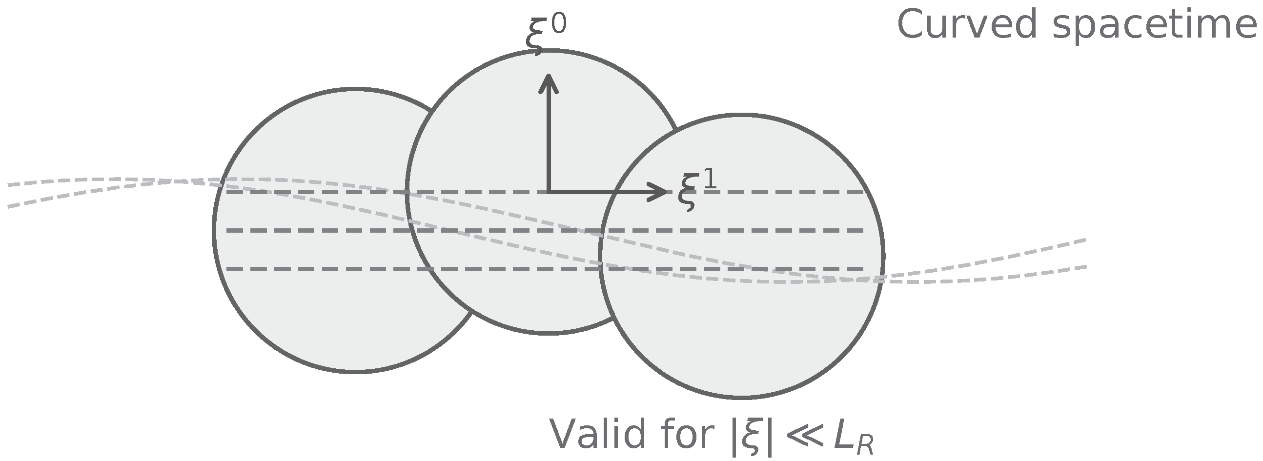
where the curvature tensor is evaluated at $x_0$. In Riemann normal coordinates centered at $x_0$, the local Minkowski patch shown in Figure 1 provides the geometric setting for this expansion. Each shaded region represents a local Minkowski patch, a convex normal neighborhood within which the metric is well approximated by Equation (2) and curvature effects are negligible. The dashed curves denote sample geodesics connecting adjacent patches, and the central arrows labeled ${\xi }^0$ and ${\xi }^1$ indicate the temporal and spatial axes of the local inertial frame centered at $x_0$. Only the ${\xi }^0$–${\xi }^1$ plane of this local coordinate system is shown.

In this local frame, a scalar or fermionic field can be expressed using a WKB-inspired ansatz. Here and below, x denotes a spacetime point (with components $x^{\mu }=(t,\mathbf{x})$ in a chosen chart), and ${\xi }^{\mu }={\xi }^{\mu }(x;x_0)$ are the associated Riemann normal (local inertial) coordinates centered at $x_0$ within a convex normal neighborhood,

$$\Phi \left(x\right)\simeq B\left(x\right)e^{iS\left(x\right)/\hslash }{\Phi }_{\mathrm{flat}}\left(\xi \left(x\right)\right),$$

(3)

where $B\left(x\right)$ is a real amplitude encoding the local transport/redshift normalization and $S\left(x\right)$ is a gravitational phase determined by the background geometry. The function ${\Phi }_{\mathrm{flat}}\left(\xi \right)$ denotes a Minkowski solution defined within each LMC patch. It satisfies the flat-space Klein–Gordon equation in Riemann normal coordinates,

$$({\square }_{\eta }+m^2){\Phi }_{\mathrm{flat}}\left(\xi \right)=0,$$

(4)

and thus represents a locally inertial mode within the patch.

Two independent small parameters control this approximation: (i) a geometric locality condition $\left|\xi \right|/L_R\ll 1$, where $L_R\sim {\left|R_{\mu \nu \rho \sigma }\right|}^{-1/2}$ sets the local curvature scale, and (ii) the semiclassical hierarchy $|{\nabla }_{\mu }B/B|\ll |{\nabla }_{\mu }S|$, since ${\nabla }_{\mu }S$ defines the local wave-vector scale $k_{\mu }$, whereas ${\nabla }_{\mu }B/B$ characterizes the much slower variation in the envelope. Together, these conditions ensure that the phase varies much more rapidly than the amplitude. When both are satisfied, the LMC framework provides a consistent procedure for embedding flat-space Feynman diagrammatics into weakly curved backgrounds.

3. Normalization, Phase, and Validity of the Local Expansion

The functions $B\left(x\right)$ and $S\left(x\right)$ follow directly from the WKB expansion of the Klein–Gordon equation. Substituting Equation (3) into $(\square +m^2)\Phi =0$ yields, schematically,

$$-{\displaystyle \frac{1}{{\hslash }^2}}{(\partial S)}^{2}B{\Phi }_{\mathrm{flat}}+{\displaystyle \frac{i}{\hslash }}\left(2{\partial }_{\mu }B{\partial }^{\mu }S+B\square S\right){\Phi }_{\mathrm{flat}}+B\left({\square }_{\eta }{\Phi }_{\mathrm{flat}}+m^2{\Phi }_{\mathrm{flat}}\right)+\dots =0,$$

(5)

where the omitted terms include additional derivatives of ${\Phi }_{\mathrm{flat}}$ and are subleading in the local WKB/LMC expansion. Using that ${\Phi }_{\mathrm{flat}}$ satisfies the flat-space Klein–Gordon equation $({\square }_{\eta }+m^2){\Phi }_{\mathrm{flat}}=0$ [Equation (4)], the terms proportional to $({\square }_{\eta }{\Phi }_{\mathrm{flat}}+m^2{\Phi }_{\mathrm{flat}})$ vanish identically. Collecting terms order by order in ℏ, the $\mathcal{O}\left({\hslash }^{-2}\right)$ contribution yields the Hamilton–Jacobi equation, while the $\mathcal{O}\left({\hslash }^{-1}\right)$ terms give the transport equation. We therefore obtain, to leading orders in ℏ,

$$\begin{array}{cc}\hfill \mathcal{O}\left({\hslash }^{-2}\right):& g^{\mu \nu }{\partial }_{\mu }S{\partial }_{\nu }S=m^2,\hfill \end{array}$$

(6)

$$\begin{array}{cc}\hfill \mathcal{O}\left({\hslash }^{-1}\right):& 2{\nabla }_{\mu }B{\partial }^{\mu }S+B\square S=0,\hfill \end{array}$$

(7)

which correspond, respectively, to the Hamilton–Jacobi (eikonal) equation for the phase $S\left(x\right)$ and the transport equation for the amplitude $B\left(x\right)$. Since $B\left(x\right)$ is a scalar function, the covariant derivative ${\nabla }_{\mu }B$ coincides with the ordinary derivative ${\partial }_{\mu }B$. The covariant notation is retained to emphasize compatibility with the curved-space divergence ${\nabla }_{\mu }{j}^{\mu }=0$.

To avoid double-counting rapid oscillations, we adopt the standard convention that all rapidly varying phase dependence is absorbed into the eikonal, while ${\Phi }_{\mathrm{flat}}$ is treated as a slowly varying (e.g., constant) polarization/spin factor over the patch. Equivalently, one may write a local Minkowski mode as

$${\Phi }_{\mathrm{flat}}\left(\xi \right)=u\left(p\right)e^{i{p}_a{\xi }^a/\hslash },p_a{p}^a=m^2,$$

(8)

where $u\left(p\right)$ denotes a constant polarization (or spinor) factor. Combining the phases into a total eikonal,

$$S_{\mathrm{tot}}\left(x\right)\equiv S\left(x\right)+p_a{\xi }^a\left(x\right),$$

(9)

Equation (3) then becomes

$$\Phi \left(x\right)\simeq B\left(x\right)e^{i{S}_{\mathrm{tot}}\left(x\right)/\hslash }u\left(p\right).$$

With this choice, the mass-shell condition is encoded in the total phase $S_{\mathrm{tot}}\left(x\right)$, whose gradient defines the local wave vector.

Derivatives acting on ${\Phi }_{\mathrm{flat}}$ do not produce independent leading-order contributions. The rapidly varying phase $e^{i{p}_a{\xi }^a/\hslash }$ has been absorbed into the total eikonal $S_{\mathrm{tot}}\left(x\right)$, so that derivatives of ${\Phi }_{\mathrm{flat}}$ no longer generate additional $\mathcal{O}\left({\hslash }^{-1}\right)$ terms. Any remaining contributions, such as derivatives of the slowly varying polarization factor $u\left(p\right)$ or corrections from the coordinate expansion ${\partial }_{\mu }{\xi }^a=e^a\mu \left(x_0\right)+\mathcal{O}\left(\right|\xi |/L_R)$, are suppressed by the locality parameter ${ϵ}_{\mathrm{curv}}\sim \left|\xi \right|/L_R$. Therefore Equations (6) and (7) are the correct leading WKB relations for the phase and amplitude in the LMC patch. This justifies the omission of such terms in the schematic expansion above.

At the bi-local level, short-distance geodesic focusing is encoded by the Van Vleck–Morette determinant

$$\Delta (x,x^{\prime })=-g^{-1/2}\left(x\right)g^{-1/2}\left(x^{\prime }\right)det\left[-{\nabla }_{\mu }{\nabla }_{{\nu }^{\prime }}\sigma (x,x^{\prime })\right],$$

(10)

where $\sigma (x,x^{\prime })$ is Synge’s world function, equal to one-half the squared geodesic distance between x and $x^{\prime }$. The dressed two-point function then has the universal Hadamard form

$$G_F(x,x^{\prime })\sim {\displaystyle \frac{{\Delta }^{1/2}(x,x^{\prime })}{4{\pi }^2(\sigma +iϵ)}}+\dots ,$$

(11)

which preserves the correct short-distance behavior in curved spacetime.

The single-point WKB factor $B\left(x\right)$ is a local transport amplitude governing external legs and local insertions, and it is conceptually distinct from the bi-local focusing factor ${\Delta }^{1/2}(x,x^{\prime })$ that appears in $G_F$. As derived below [see Equation (16)], along null geodesics one finds $B^2\propto {\Delta }^{1/2}$ (with the standard Van Vleck convention), so that B encodes the square-root of the local flux transport, while ${\Delta }^{1/2}$ encodes the full geodesic focusing of the two-point function.

In a stationary-phase evaluation of vertex integrals, the Hessian determinant at the geodesic saddle combines with the local Jacobian $|\partial \xi /\partial x|$ to reproduce the Van Vleck factor ${\Delta }^{1/2}(x,x^{\prime })$, ensuring a consistent leading-order matching between adjacent patches without double-counting transport effects.

It is useful to make precise the relation between the single-point transport factor $B\left(x\right)$ and the bi-local Van Vleck determinant $\Delta (x,x^{\prime })$ along a null geodesic congruence. Let $k^{\mu }\equiv {\nabla }^{\mu }S$ denote the (null) wave vector and $\lambda$ an affine parameter along the geodesics, so that $k^{\mu }{\nabla }_{\mu }=\mathrm{d}/\mathrm{d}\lambda$. Contracting the transport Equation (7) with $k^{\mu }$ and using $\square S={\nabla }_{\mu }{k}^{\mu }$ gives

$$k^{\mu }{\nabla }_{\mu }B+\frac{1}{2}B{\nabla }_{\mu }{k}^{\mu }=0\Rightarrow {\displaystyle \frac{\mathrm{d}}{\mathrm{d}\lambda }}lnB=-{\displaystyle \frac{1}{2}}\theta \left(\lambda \right),$$

(12)

where $\theta \equiv {\nabla }_{\mu }{k}^{\mu }$ is the expansion of the null congruence. Hence

$$B\left(\lambda \right)\propto exp\left(-\frac{1}{2}{\int }^{\lambda }\theta \left(\tilde{\lambda }\right)\mathrm{d}\tilde{\lambda }\right).$$

(13)

The Van Vleck determinant $\Delta (x,x^{\prime })$ encodes the infinitesimal change in transverse geodesic separation and satisfies the transport law (in the usual convention for $\Delta$)

$$k^{\mu }{\nabla }_{\mu }ln{\Delta }^{1/2}=-\theta \left(\lambda \right),$$

(14)

so that

$${\Delta }^{1/2}\left(\lambda \right)\propto exp\left(-{\int }^{\lambda }\theta \left(\tilde{\lambda }\right)\mathrm{d}\tilde{\lambda }\right).$$

(15)

Comparing Equations (13) and (15) yields the relation (with the standard Van Vleck convention used in Equation (14))

$$B^2\left(\lambda \right)\propto {\Delta }^{1/2}\left(\lambda \right)\Rightarrow B\left(\lambda \right)\propto {\Delta }^{1/4}\left(\lambda \right).$$

(16)

We emphasize two points. First, the proportionality constants above are fixed by initial (or matching) data at the chosen patch center and by the chosen normalization of local Minkowski modes. They are not encoded in the local transport equations. Second, statements of the form “$B\propto {\Delta }^{\alpha }$” must specify the convention for $\Delta$ explicitly. With the standard convention used in the Hadamard parametrix, the appropriate power is $\alpha =\frac{1}{4}$, as shown in Equation (16). The prior phrasing in the manuscript that “$B\propto {\Delta }^{1/2}$” therefore conflates different normalization conventions and is replaced by the corrected, convention-explicit relation above.

For null propagation, the transport equation reduces to

$${\nabla }_{\mu }\left(B^2{k}^{\mu }\right)=0,k^{\mu }={\nabla }^{\mu }S,$$

with $k^{\mu }$ the local wave vector. The precise relation between B and the Van Vleck determinant is derived below [see Equation (16)]. Hence, even in the massless limit, the amplitude varies along the null congruence according to its expansion $\theta ={\nabla }_{\mu }{k}^{\mu }$, rather than remaining constant. The conserved current,

$$j^{\mu }={\displaystyle \frac{i}{2\hslash }}\left({\Phi }^{\ast }{\nabla }^{\mu }\Phi -\Phi {\nabla }^{\mu }{\Phi }^{\ast }\right)=B^2{\partial }^{\mu }S,$$

(17)

satisfies ${\nabla }_{\mu }{j}^{\mu }=0$, confirming that $B\left(x\right)$ acts as a local normalization ensuring covariant flux conservation along the classical flow defined by $S\left(x\right)$.

Substituting the ansatz (3) into the current (17) yields

$$j^{\mu }=B^2{\left|{\Phi }_{\mathrm{flat}}\left(\xi \right)\right|}^2{\partial }^{\mu }S+\mathcal{O}\left({ϵ}_{\mathrm{curv}}\right),$$

(18)

up to subleading terms suppressed by derivatives of the slowly varying polarization factor. In the LMC construction, ${\Phi }_{\mathrm{flat}}\left(\xi \right)$ represents a locally normalized Minkowski mode inside the patch. Its modulus is therefore constant over the convex normal neighborhood and may be absorbed into the normalization of the one-particle state. With this standard normalization choice, $|{\Phi }_{\mathrm{flat}}{|}^2=1$, and the current reduces to

$$j^{\mu }=B^2{\partial }^{\mu }S,$$

(19)

as used in Equation (17).

For a static metric with

$$d{s}^2=-f\left(r\right)d{t}^2+f^{-1}\left(r\right)d{r}^2,$$

(20)

inserting

$$S=\omega t-\int dr(\omega /f)$$

(21)

into Equation (7) gives

$$B\propto f^{-1/4}={(-g_{00})}^{-1/4}.$$

(22)

Equation (22) represents the redshift normalization factor associated with the time–radial sector of the metric and the choice of static observers. In a full four-dimensional Schwarzschild spacetime, additional geometric effects such as angular spreading of wavefronts and greybody transmission factors further influence the amplitude of radiative modes. These global and geometric effects are not captured by the local normalization factor $B\left(r\right)$ and are treated separately in standard analyses. In the present framework, $B\left(r\right)$ should therefore be interpreted strictly as the local redshift normalization entering the WKB transport equation, rather than as the complete radial dependence of physical fluxes. It represents a local normalization factor rather than a global enhancement of radiative power or particle number. When integrated over a complete hypersurface, the conserved flux derived from $j^{\mu }$ remains invariant, ensuring consistency with global energy conservation.

The LMC framework relies on the assumption that curvature effects can be treated perturbatively inside each local patch. The expansion in Equation (2) is valid as long as

$${\left|\xi \right|}^2\ll {\displaystyle \frac{1}{|R_{\alpha \beta \gamma \delta }\left(x_0\right)|}},$$

(23)

so that higher-order terms involving curvature derivatives remain negligible.

To quantify the range of validity, it is convenient to introduce dimensionless expansion parameters,

$${ϵ}_{\mathrm{curv}}={\displaystyle \frac{{\mathcal{l}}_{\mathrm{wave}}}{L_R}},{ϵ}_{\mathrm{grad}}={\displaystyle \frac{{\mathcal{l}}_{\mathrm{wave}}}{L_{\nabla R}}},{ϵ}_{\mathrm{int}}=\lambda {\mathcal{l}}_{\mathrm{wave}}^2{E}^2,$$

(24)

where ${\mathcal{l}}_{\mathrm{wave}}\sim E^{-1}$ is the typical wavelength, $L_R\sim {\left|R_{\mu \nu \rho \sigma }\right|}^{-1/2}$ the curvature radius, and $L_{\nabla R}\sim {|\nabla R_{\mu \nu \rho \sigma }|}^{-1/3}$ the scale of curvature variation. The LMC expansion is reliable provided ${ϵ}_{\mathrm{curv}},{ϵ}_{\mathrm{grad}},{ϵ}_{\mathrm{int}}\ll 1$. For a $10M_{\odot }$ black hole, using $L_R\sim {\left|R\right|}^{-1/2}$ with $\left|R\right|=\sqrt{48}GM/r^3$, one finds $L_R\approx 2.9\times {10}^4\mathrm{m}$ at $r=3GM$, implying ${ϵ}_{\mathrm{curv}}\sim 7\times {10}^{-21}$ for GeV scale quanta. For Schwarzschild, the Kretschmann scalar is $K\equiv R_{\mu \nu \rho \sigma }{R}^{\mu \nu \rho \sigma }=48G^2{M}^2/r^6$. With our norm $\left|R\right|\equiv \sqrt{K}$, the curvature radius is

$$L_R\sim {\left|R\right|}^{-1/2}={\displaystyle \frac{r^{3/2}}{{48}^{1/4}\sqrt{GM}}}.$$

(25)

At $r=6GM$ and $M=10M_{\odot }$, using Equation (25) to evaluate the curvature radius $L_R$, one finds $L_R\approx 8.2\times {10}^4\mathrm{m}$ ($\approx 82\mathrm{km}$). The Hawking temperature corresponds to the angular frequency ${\omega }_H=k_B{T}_H/\hslash =c^3/\left(8\pi GM\right)$ (here, the speed of light c is restored for numerical estimates). Numerically ${\omega }_H\approx 8.1\times {10}^2{\mathrm{s}}^{-1}$ for $10M_{\odot }$, so the reduced wavelength is ${\mathcal{l}}_{\mathrm{wave}}\sim c/{\omega }_H\approx 3.7\times {10}^5\mathrm{m}$. Hence

$${ϵ}_{\mathrm{curv}}={\displaystyle \frac{{\mathcal{l}}_{\mathrm{wave}}}{L_R}}\approx {\displaystyle \frac{3.7\times {10}^5\mathrm{m}}{8.2\times {10}^4\mathrm{m}}}\approx 4.5(r=6GM,\omega \sim {\omega }_H),$$

(26)

indicating that the geometric-optics/WKB expansion is not yet parametrically small for quanta at the thermal peak so deep in the potential. For higher energies or farther out the expansion improves rapidly: at $r=10GM$ one has $L_R\simeq 1.77\times {10}^5\mathrm{m}$, giving ${ϵ}_{\mathrm{curv}}\approx 0.21$ for $\omega =10{\omega }_H$ (and ≈0.11 for $\omega =20{\omega }_H$). These estimates quantify where the LMC/WKB treatment is accurate: either for quanta with $\omega \gg {\omega }_H$ or at radii where $L_R$ is larger (weaker curvature), consistent with the conditions in Equations (25)–(28).

In what follows we require a quantitative small parameter

$$\epsilon \left(x\right)\equiv {\displaystyle \frac{{\lambda }_{\mathrm{ph}}\left(x\right)}{L_{\mathrm{curv}}\left(x\right)}}\lesssim 0.3,$$

(27)

so that subleading transport/Hadamard terms remain controlled. Accordingly, all statements and plots are restricted to radii/frequencies satisfying Equation (27). Near $r\approx 6GM$ at $\omega \sim {\omega }_H$ the expansion is not parametrically small and results are qualitative only.

In black-hole spacetimes, Equation (22) formally diverges as $g_{00}\to 0$, signaling the breakdown of the local expansion rather than a physical infinity. The method should therefore be restricted to regions satisfying

$${\mathcal{l}}_{\mathrm{patch}}\ll L_R,$$

(28)

where ${\mathcal{l}}_{\mathrm{patch}}$ denotes the characteristic size of the local Riemann normal neighborhood. Otherwise geodesic convergence and strong-field effects invalidate the Riemann normal coordinate expansion. Outside convex normal neighborhoods, multiple geodesics or conjugate points can occur and ${\Delta }^{1/2}(x,x^{\prime })$ may vanish. In such regions the present leading-order LMC description must be patched across saddles (including the appropriate Maslov phases) or replaced by a full Hadamard expansion.

Condition (28) should be understood as a geometric requirement ensuring that the local Riemann normal expansion remains valid within a convex normal neighborhood and that geodesic focusing does not invalidate the WKB hierarchy. In practice, the operative control parameters of the LMC expansion are the local smallness conditions $\left|\xi \right|\ll L_R$ and $\epsilon \equiv {\lambda }_{\mathrm{ph}}/L_{\mathrm{curv}}\ll 1$, as defined in Equation (27). For sufficiently high-frequency modes, these conditions may remain satisfied closer to the horizon, while for modes near the Hawking scale the breakdown occurs earlier. All results presented here are restricted to regions where these local control parameters remain small.

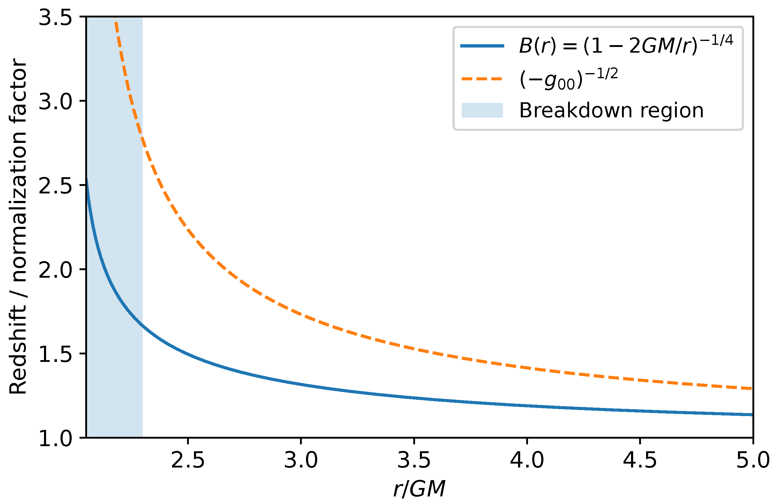
The radial behavior of the local normalization function $B\left(r\right)$, together with the Tolman redshift factor ${(-g_{00})}^{-1/2}$, is shown in Figure 2. Both functions increase sharply as $r\to 2GM$, reflecting the gravitational redshift of static coordinates in the static frame. The divergence is not physical but marks the limit of applicability of the WKB and Riemann normal expansions. Beyond this region, the local LMC approximation fails.

When these locality and hierarchy conditions are fulfilled, the LMC construction provides a reliable and computationally efficient framework for calculating curvature-sensitive amplitudes in weakly curved backgrounds while remaining consistent with standard semiclassical physics.

4. Curvature-Modified Feynman Rules and Example

Within the LMC framework, the standard Feynman diagram expansion retains its topological structure, while curvature effects appear through multiplicative factors derived from the normalization function $B\left(x\right)$ and the gravitational phase $S\left(x\right)$. For scalar and spinor fields, we write

$$\Phi \left(x\right)=B\left(x\right)e^{iS\left(x\right)/\hslash }{\Phi }_{\mathrm{flat}}\left(\xi \left(x\right)\right),\Psi \left(x\right)=B\left(x\right)e^{iS\left(x\right)/\hslash }{\psi }_{\mathrm{flat}}\left(\xi \left(x\right)\right),$$

(29)

where ${\Phi }_{\mathrm{flat}}$ is the scalar field introduced in Section 2, and ${\psi }_{\mathrm{flat}}$ denotes the corresponding flat-space spinor field expressed in Riemann normal coordinates. The corresponding scalar propagator in a convex normal neighborhood is taken in Hadamard form,

$$G_F(x,x^{\prime })={\displaystyle \frac{i}{8{\pi }^2}}\left[{\displaystyle \frac{U(x,x^{\prime })}{\sigma (x,x^{\prime })+iϵ}}+V(x,x^{\prime })ln\left({\mu }^2[\sigma (x,x^{\prime })+iϵ]\right)+W(x,x^{\prime })\right],$$

(30)

with $U(x,x^{\prime })={\Delta }^{1/2}(x,x^{\prime })$ the Van Vleck–Morette biscalar, $V(x,x^{\prime })$ a smooth biscalar determined by the local geometry, and $W(x,x^{\prime })$ encoding the state-dependent regular part of the two-point function. Here $\sigma (x,x^{\prime })$ is Synge’s world function. This form reproduces the universal short-distance singular structure of two-point functions in curved spacetime. No single-point normalization factors $B(·)$ appear in $G_F$; all observer-dependent normalizations are assigned to external legs, as discussed below under external legs and observer frames. Here ${\Delta }^{1/2}(x,x^{\prime })$ carries the bi-local geodesic focusing. It is not duplicated by the single-point transport factors $B\left(x\right),B\left(x^{\prime }\right)$. Equation (30) is valid only inside convex normal neighborhoods, where $S\left(x\right)$ remains single-valued and $\xi \left(x\right)$ and $\xi \left(x^{\prime }\right)$ are connected by a unique geodesic. The multiplicative factors $B_u\left(x\right)$ and $S\left(x\right)$ act as a local dressing of propagators and external lines, while the diagram topology and combinatorics remain unchanged.

For a Yukawa interaction, we use the usual curved-space vertex density with invariant measure,

$${\mathcal{L}}_{\mathrm{int}}\left(x\right)=\lambda \overline{\Psi }\left(x\right)\Phi \left(x\right)\Psi \left(x\right),\int d^{4}x\sqrt{-g\left(x\right)}{\mathcal{L}}_{\mathrm{int}}\left(x\right).$$

(31)

Vertices carry no additional B factors; the invariant measure $\sqrt{-g}{d}^{4}x$ and the bi-local structure of $G_F$ already encode the geometric effects. Observer-dependent normalizations $B_u$ appear only on external legs, as discussed below.

All vertex integrals are evaluated with the curved-space measure $\sqrt{-g\left(x\right)}{d}^{4}x$, or equivalently $|\partial \xi /\partial x|d^4\xi$ in local coordinates. When stationary-phase approximations are used to match adjacent patches, the corresponding Jacobian factors ensure that the overall normalization of amplitudes remains covariant. In a stationary-phase evaluation of the vertex integrals, ${\partial }_{\xi }[S\left(x\right)-S\left(x^{\prime }\right)]=0$ selects the geodesic saddle. The resulting Hessian determinant combines with $|\partial \xi /\partial x|$ to yield the Van Vleck determinant ${\Delta }^{1/2}(x,x^{\prime })$, ensuring a consistent leading-order matching between patches.

To make the origin of the LMC rules explicit, we briefly outline their derivation from the curved-space action. For simplicity, we take $\Phi$ to be a real scalar field, so that the interaction Lagrangian is manifestly Hermitian. The extension to complex scalar fields is direct and does not affect the WKB transport equations or the structure of the LMC construction (see, e.g., Refs. [1,2]). For definiteness, consider a scalar–fermion Yukawa theory with action

$$S=\int d^{4}x\sqrt{-g}\left[\overline{\Psi }(i{\gamma }^{\mu }{D}_{\mu }-m_{\psi })\Psi +{\displaystyle \frac{1}{2}}{g}^{\mu \nu }{\partial }_{\mu }\Phi {\partial }_{\nu }\Phi -{\displaystyle \frac{1}{2}}{m}_{\varphi }^2{\Phi }^2-\lambda \overline{\Psi }\Phi \Psi \right].$$

(32)

Here $D_{\mu }$ denotes the spinor covariant derivative (including the spin connection), and ${\gamma }^{\mu }=e_a^{\mu }{\gamma }^a$ are the curved-space Dirac matrices. Inside a convex normal neighborhood we insert the LMC decomposition

$$\Phi \left(x\right)=B\left(x\right)e^{iS\left(x\right)/\hslash }{\Phi }_{\mathrm{flat}}\left(\xi \left(x\right)\right),\Psi \left(x\right)=B\left(x\right)e^{iS\left(x\right)/\hslash }{\psi }_{\mathrm{flat}}\left(\xi \left(x\right)\right).$$

(33)

The quadratic part of the action determines the propagators. To leading WKB order, the phase $S\left(x\right)$ satisfies the Hamilton–Jacobi equation, while the transport equation ensures ${\nabla }_{\mu }\left(B^2{\nabla }^{\mu }S\right)=0$. After factoring out the local phase and normalization, the remaining quadratic operator acting on ${\Phi }_{\mathrm{flat}}$ and ${\psi }_{\mathrm{flat}}$ reduces to the standard Minkowski operator in Riemann normal coordinates, up to subleading corrections.

Terms involving derivatives of $B\left(x\right)$ beyond the transport equation are suppressed by the semiclassical hierarchy $|{\nabla }_{\mu }B/B|\ll |{\nabla }_{\mu }S|$ and by the locality expansion ${ϵ}_{\mathrm{curv}}\sim \left|\xi \right|/L_R\ll 1$. Consequently, such terms do not contribute at leading WKB order. Therefore, the internal propagators are given by the standard curved-space Hadamard two-point functions determined by the quadratic action, without additional single-point $B\left(x\right)$ factors.

For interaction terms, each vertex contributes

$$\int d^{4}x\sqrt{-g}\lambda \overline{\Psi }\left(x\right)\Phi \left(x\right)\Psi \left(x\right).$$

(34)

The invariant measure $\sqrt{-g}{d}^{4}x$ already accounts for the geometric Jacobian. Since the $B\left(x\right)e^{iS\left(x\right)/\hslash }$ factors are associated with external wavefunctions and Lehmann–Symanzik–Zimmermann (LSZ) reduction [10], they are not attached to internal propagators. Instead, they appear only in the external-leg normalization when amplitudes are evaluated between locally normalized one-particle states. Thus, to leading order in the LMC expansion,

• internal lines are given by the standard curved-space Hadamard propagators determined by the quadratic action,
• vertices are integrated with the invariant measure $\sqrt{-g}{d}^{4}x$,
• external legs acquire the observer-dependent normalization and phase factors $B_u\left(x\right)e^{iS\left(x\right)/\hslash }$.

This establishes the LMC Feynman rules as a direct consequence of the action and LSZ reduction within each local patch.

Having established these ingredients, the curvature-dressed version of flat-space perturbation theory can be summarized by the following modified Feynman (LMC) rules:

• Internal propagators: Use the Hadamard form (30) with $U={\Delta }^{1/2}$. Do not attach any single-point B factors to $G_F$.
• Vertices: Integrate with the invariant measure $\int d^{4}x\sqrt{-g}{\mathcal{L}}_{\mathrm{int}}\left(x\right)$; no extra B factors at vertices.
• External legs (observer-dependent): If amplitudes are defined with respect to an observer congruence $u^{\mu }$, attach

  $${\Phi }_{\mathrm{ext}}\left(x\right)\to B_u\left(x\right){\Phi }_{\mathrm{ext}}\left(x\right),B_u\left(x\right)={\left({\displaystyle \frac{{\omega }_{\mathrm{loc}}\left(x\right)}{{\omega }_{\infty }}}\right)}^{-1/2},{\omega }_{\mathrm{loc}}\left(x\right)\equiv -u^{\mu }{k}_{\mu }.$$
  For static observers, $B_u\left(x\right)={(-g_{00})}^{-1/4}$.
• Patching/caustics: When multiple geodesics connect x and $x^{\prime }$, sum saddle contributions, each with its own ${\Delta }^{1/2}$, and include the Maslov phase $e^{-i\pi \mu /2}$ per conjugate point.

These rules together provide a self-consistent prescription for constructing amplitudes within each LMC patch. In some heuristic implementations of local WKB dressing (see, e.g., Ref. [8]), single-point factors of the form $B\left(x\right)B\left(x^{\prime }\right)$ have been attached directly to propagators. Since the bi-local Hadamard coefficient $U(x,x^{\prime })={\Delta }^{1/2}(x,x^{\prime })$ already encodes geodesic focusing, such additional factors would duplicate transport effects. In the present formulation, single-point normalization factors are therefore assigned only to external legs. Accordingly, within the LMC approximation, the observer-dependent normalization factor $B_u\left(x\right)$ is assigned to external legs only. The factor $B_u\left(x\right)$ is distinct from the WKB amplitude $B\left(x\right)$ and represents the observer-dependent normalization of external states, while internal propagators retain their standard curved-space Hadamard structure. These rules retain the flat-space diagrammatic structure while incorporating gravitational redshift and phase effects. They enable local, curvature-sensitive amplitude calculations without requiring global mode expansions or a preferred vacuum state.

We now clarify the observer-dependent normalization factor that appears on external legs. Let $u^{\mu }\left(x\right)$ be a timelike unit vector field (observer congruence) with local tetrad ${e_a}^{\mu }$. Mode amplitudes normalized with respect to observer proper time $\tau$ scale as ${\left(2{\omega }_{\mathrm{loc}}\right)}^{-1/2}$, with ${\omega }_{\mathrm{loc}}\left(x\right)\equiv -u^{\mu }{k}_{\mu }\left(x\right)$. If asymptotic particle definitions use a Killing time t (where it exists), then ${\omega }_{\infty }\equiv -{\xi }^{\mu }{k}_{\mu }$ and, in static regions, ${\omega }_{\mathrm{loc}}={\omega }_{\infty }/\sqrt{-{\xi }^2\left(x\right)}$ (Tolman relation). Thus

$$B_u\left(x\right)\equiv {\left(\frac{{\omega }_{\mathrm{loc}}\left(x\right)}{{\omega }_{\infty }}\right)}^{-1/2},\mathrm{so}\mathrm{that}{B}_{\mathrm{static}}\left(x\right)={\left(-g_{00}\left(x\right)\right)}^{-1/4}.$$

(35)

$B_u$ is observer-dependent and therefore does not belong to covariant bi-local objects like $G_F(x,x^{\prime })$. We assign $B_u$ solely to external legs and local measurements.

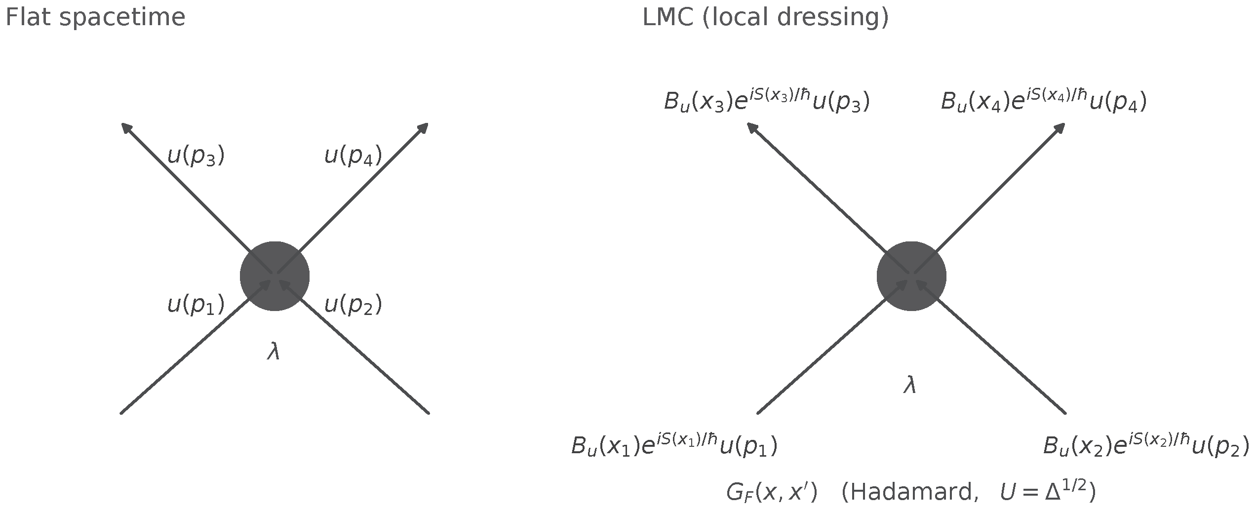
As a concrete example illustrating the use of the LMC rules, we consider tree-level fermion–fermion scattering via scalar exchange in a weakly curved background. The corresponding diagrams are shown in Figure 3. The left panel represents the standard tree-level Yukawa vertex in flat spacetime, while the right panel illustrates the same process in the LMC framework. In the LMC framework, curvature dependence enters amplitudes through observer-dependent external-leg normalization factors and local phase accumulation, while internal propagators retain their standard curved-spacetime Hadamard form. Vertices are integrated with the invariant measure $\sqrt{-g}{d}^{4}x$ and do not carry additional single-point normalization factors. This separation avoids double-counting of transport effects already encoded in the Van Vleck–Morette determinant and ensures consistency with covariant flux conservation.

These curvature-dependent terms encode redshift and phase effects locally but do not change the topology of the Feynman diagram. In flat spacetime, the amplitude is

$${\mathcal{M}}_{\mathrm{flat}}=-i{\lambda }^2\overline{u}\left(p_3\right)u\left(p_1\right){\displaystyle \frac{1}{{(p_1+p_2)}^2-m^2+iϵ}}\overline{u}\left(p_4\right)u\left(p_2\right).$$

(36)

To make the representation explicit, it is convenient to write the tree-level amplitude in coordinate space before Fourier transformation. In flat spacetime the connected four-point function reads schematically

$$\begin{array}{ccc}\hfill {\mathcal{A}}_{\mathrm{flat}}(x_1,x_2,x_3,x_4)& =& {(-i\lambda )}^2\int d^{4}x{d}^4{x}^{\prime }\overline{u}\left(p_3\right)S_F(x_3,x)S_F(x,x_1)G_F(x,x^{\prime })\hfill \\ & & \times S_F(x^{\prime },x_2)S_F(x_4,x^{\prime })u\left(p_1\right)u\left(p_2\right).\hfill \end{array}$$

(37)

Here $A_{\mathrm{flat}}(x_1,x_2,x_3,x_4)$ denotes the flat-space four-point amplitude written in local inertial coordinates within the patch, prior to LSZ reduction. The dependence on momenta $p_i$ enters through the choice of external one-particle states, represented by the spinors $u\left(p_i\right)$, while the propagators $G_F$ and $S_F$ are written in coordinate space, with $G_F$ taken in Hadamard form, Equation (30). The fermion propagator $S_F(x,x^{\prime })$ is defined as the Green’s function of the Dirac operator,

$$(i{\gamma }^{\mu }{D}_{\mu }-m_{\psi })S_F(x,x^{\prime })={\displaystyle \frac{{\delta }^{\left(4\right)}(x,x^{\prime })}{\sqrt{-g}}}.$$

The spinors $u\left(p_i\right)$ represent external on-shell states and, in this representation, are independent of the spacetime coordinates. In the LMC framework, curvature modifies only the local normalization and phase of the external legs, while internal propagators retain their standard curved-space Hadamard form. Thus the coordinate-space amplitude takes the leading-order LMC form

$${\mathcal{A}}_{\mathrm{LMC}}\left(x_i\right)=\prod _{i=1}^4\left[B_u\left(x_i\right)e^{iS\left(x_i\right)/\hslash }\right]{\mathcal{A}}_{\mathrm{flat}}\left(x_i\right)+\mathcal{O}\left({ϵ}_{\mathrm{curv}}\right),$$

(38)

where ${\mathcal{A}}_{\mathrm{flat}}\left(x_i\right)$ denotes the flat-space amplitude expressed in local inertial coordinates within the patch.

The usual momentum-space amplitude $M_{\mathrm{flat}}\left(p_i\right)$ is obtained from ${\mathcal{A}}_{\mathrm{flat}}\left(x_i\right)$ by LSZ reduction and Fourier transformation with respect to asymptotic plane-wave modes. In this procedure the external-leg normalization factors $B_u\left(x_i\right)$ are absorbed into the definition of locally normalized one-particle states. Consequently, the schematic expression

$$M_{\mathrm{LMC}}=\prod _{i=1}^4{B}_u\left(x_i\right)e^{iS\left(x_i\right)/\hslash }{M}_{\mathrm{flat}}$$

(39)

should be understood as shorthand for the coordinate-space dressing (38) prior to LSZ reduction, rather than as a literal multiplication of a momentum-space amplitude by coordinate-dependent functions.

The curvature dependence appearing in Equation (38) modifies the local normalization and phase structure of amplitudes inside each LMC patch, but it does not alter globally conserved observables once the proper redshift and LSZ normalization factors are taken into account. In particular, when amplitudes are evaluated between asymptotic states defined with respect to a fixed observer congruence, the external-leg factors $B_u\left(x\right)$ are absorbed into the normalization of one-particle states. The formalism therefore changes the local representation of Feynman diagrams without modifying physical S-matrix elements or globally conserved fluxes, ensuring consistency with semiclassical energy conservation.

The invariance of global observables can be seen directly from the conserved current. From Equation (19) one has

$$j^{\mu }=B^2\left(x\right){\partial }^{\mu }S\left(x\right),$$

(40)

where $k^{\mu }={\nabla }^{\mu }S$ defines the local wave vector, with locally measured frequency ${\omega }_{\mathrm{loc}}=-u_{\mu }{k}^{\mu }$. Identifying the WKB amplitude $B\left(x\right)$ with the observer-dependent normalization factor $B_u\left(x\right)\propto {\omega }_{\mathrm{loc}}^{-1/2}$, one obtains

$$B^2\left(x\right)\propto {\omega }_{\mathrm{loc}}^{-1}.$$

(41)

Hence the current scales as

$$j^{\mu }\propto {\omega }_{\mathrm{loc}}^{-1}{\omega }_{\mathrm{loc}}=\mathrm{constant}$$

(42)

along the classical flow.

This shows explicitly that the position-dependent normalization factors entering Equation (38) do not modify conserved fluxes: the redshift of local energy is exactly compensated by the normalization of external states. When amplitudes are expressed in terms of asymptotic frequencies ${\omega }_{\infty }$ via LSZ reduction, all local factors $B_u\left(x\right)$ cancel, and the resulting S-matrix elements coincide with their standard curved-spacetime counterparts.

While the normalization factors cancel in globally conserved observables, the gravitational phase $S\left(x\right)$ still affects local amplitudes through relative phase differences. This effect is most transparent in processes receiving contributions from more than one local emission region or stationary-phase saddle. If two such contributions arise from two spacetime points $x_a$ and $x_b$ within the domain of validity of the patchwise construction, the leading-order dressed amplitude takes the schematic form

$${\mathcal{A}}_{\mathrm{LMC}}\sim B_u\left(x_a\right)e^{iS\left(x_a\right)/\hslash }{\mathcal{A}}_a+B_u\left(x_b\right)e^{iS\left(x_b\right)/\hslash }{\mathcal{A}}_b,$$

(43)

where ${\mathcal{A}}_{a,b}$ denote the corresponding flat-space reduced amplitudes in local inertial coordinates. The resulting probability then contains the interference term

$$|{\mathcal{A}}_{\mathrm{LMC}}{|}^2\supset 2B_u\left(x_a\right)B_u\left(x_b\right)\mathrm{Re}\left[{\mathcal{A}}_a{\mathcal{A}}_b^{\ast }{e}^{i\left(S\left(x_a\right)-S\left(x_b\right)\right)/\hslash }\right].$$

(44)

Thus curvature enters not only through the local normalization factors $B_u\left(x\right)$ but also through the relative phase difference $S\left(x_a\right)-S\left(x_b\right)$ accumulated along the relevant geodesic branches. In this way, the LMC rules predict curvature-modulated interference patterns at the level of local amplitudes, even though the global normalization of conserved fluxes remains unchanged.

5. Applications and Phenomenology

We now apply the LMC formalism to describe local pair creation in the vicinity of a Schwarzschild horizon. This analysis parallels the standard Hawking process but is formulated entirely in terms of locally defined amplitudes. The Schwarzschild metric,

$$d{s}^2=-\left(1-{\displaystyle \frac{2GM}{r}}\right)d{t}^2+{\left(1-{\displaystyle \frac{2GM}{r}}\right)}^{-1}d{r}^2+r^{2}d{\Omega }^2,$$

(45)

admits a local inertial frame near any point $r_0>2GM$. From Equation (22), the normalization function becomes

$$B\left(r\right)={\left(1-{\displaystyle \frac{2GM}{r}}\right)}^{-1/4},$$

(46)

which diverges formally as $r\to 2GM$. This divergence reflects the infinite redshift of static coordinates and marks the limit of validity of the local approximation rather than a physical divergence.

Schematic pair-creation amplitudes then take the form of local integrals of Hadamard two-point functions along with external-leg normalizations $B_u$ appropriate to the chosen observer congruence.

To connect these local amplitudes with physical observables, we now consider the resulting flux at asymptotic infinity. Within the LMC framework, the assignment of local normalization and phase factors is such that, when the global two-point function corresponds to the Unruh state, the standard point-splitting calculation reproduces the usual Hawking flux at ${\mathcal{I}}^{+}$.

We sketch a stress-tensor check consistent with the Unruh vacuum. Using point-splitting with Hadamard subtraction, the renormalized flux component at future null infinity is

$${\langle T_{uu}\rangle }_{\mathrm{ren}}=\underset{x^{\prime }\to x}{lim}{\mathcal{D}}_{uu}\left[G_F(x,x^{\prime })-G_H(x,x^{\prime })\right],$$

(47)

where u is an affine retarded null coordinate, $G_F$ is the exact two-point function in the Unruh state, $G_H$ the local Hadamard parametrix with $U={\Delta }^{1/2}$, and ${\mathcal{D}}_{uu}$ the standard bi-differential operator for $T_{uu}$. In the near-horizon region, modes normalized with respect to static observers pick up the Tolman factor in their external-leg normalization, $B_{\mathrm{static}}={(-g_{00})}^{-1/4}$, while the bi-local singular structure is fixed entirely by $U={\Delta }^{1/2}$ in (30). Propagating to ${\mathcal{I}}^{+}$, the redshift of frequency ${\omega }_{\mathrm{loc}}={\omega }_{\infty }/\sqrt{-g_{00}}$ is exactly compensated by the external-leg normalization $B_{\mathrm{static}}$, so the renormalized flux at infinity retains the Unruh value,

$${\langle T_{uu}\rangle }_{{\mathcal{I}}^{+}}={\displaystyle \frac{\pi }{12}}{T}_H^2(\mathrm{per}\mathrm{scalar}\mathrm{d}.\mathrm{o}.\mathrm{f}.),$$

(48)

with $T_H=\kappa /\left(2\pi \right)$. This result follows from the standard relation ${\langle T_{uu}\rangle }_{{\mathcal{I}}^{+}}=(\pi /12)T_H^2$ for the Unruh vacuum, confirming that the LMC normalization assignment does not alter the conserved flux once redshift and proper-time normalization are accounted for. Greybody factors are encoded by the global radial wave operator and remain unchanged by our bookkeeping (since internal lines use the standard $G_F$ in Hadamard form). This establishes that the LMC assignment–$B_u$ on external legs only, with $G_F$ bi-locally Hadamard–is consistent with the Hawking flux in the Unruh state.

The factors $B^n\left(x\right)$ represent only the redshift normalization of local amplitudes. When the radiation is propagated to asymptotic infinity, the redshift of energy exactly compensates for the local amplitude scaling, leaving the overall Hawking flux unchanged. The LMC framework therefore reproduces the standard Hawking result while providing a transparent local interpretation of the underlying processes.

The curvature-dependent normalization function $B\left(x\right)$ influences how field amplitudes are expressed in curved backgrounds but does not alter the total emission rate observed at infinity. In this sense, the LMC formalism provides a refined local description without modifying Hawking’s global result. It should be emphasized that the LMC construction itself does not determine the quantum state; the agreement with the Hawking flux follows only when the Unruh state is adopted as the global boundary condition.

Close to the horizon, the breakdown of the WKB expansion (where $g_{00}\to 0$) sets a natural cutoff for the applicability of Equation (46). Within its range of validity, the formalism describes a spatial redistribution of local field amplitudes that, in principle, may be probed in analog-gravity experiments. Systems such as Bose–Einstein condensates and optical waveguides, where effective horizons can be engineered, may provide accessible laboratory platforms to study curvature-modulated amplitude profiles and interference effects, as discussed in analog-gravity systems [11].

Although the LMC factors $B\left(x\right)$ and $S\left(x\right)$ can be used to parameterize the spectrum locally, any interpretation of an “effective temperature” must be viewed as phenomenological rather than fundamental. The true Hawking temperature remains $T_{\mathrm{H}}=1/\left(8\pi GM\right)$, determined by the surface gravity of the black hole.

Overall, the LMC framework supplies a conceptually clear and computationally efficient way to treat quantum processes in weakly curved spacetimes while maintaining consistency with the established semiclassical picture of black-hole radiation.

6. Relation to Existing Frameworks

Several recent studies have explored local formulations of quantum field theory in curved spacetime that share conceptual similarities with the LMC approach. Li [8] proposed a WKB-based expansion in Riemann normal coordinates to study scalar and spinor propagation in weak gravitational fields, while MacKay [9] analyzed the consistency of this construction and identified the range where the weak-field approximation remains reliable.

It is worth noting that the use of local inertial (Minkowski) coordinates in quantization has been discussed extensively in the context of de Sitter space, where different choices of vacuum can lead to physically distinct results. In particular, quantization based purely on Local Minkowski Coordinates and analytic continuation in proper time has been argued to lead to instabilities, whereas quantization based on global symmetries selects the Bunch–Davies vacuum, which is stable. This distinction can be understood in terms of the choice of $iϵ$ prescription and, more generally, of the global quantum state.

In the present work, the LMC construction is local by design and does not itself fix the global quantum state. Physical predictions therefore depend on the choice of state used to define asymptotic observables. When a standard choice (such as the Unruh state in black-hole spacetimes) is adopted, the LMC framework remains fully consistent with established semiclassical results.

The present work extends these ideas into a complete diagrammatic framework that integrates curvature effects directly into the building blocks of perturbative quantum field theory. Unlike earlier qualitative analyses, the LMC formulation provides explicit Feynman rules in which curvature enters through the observer-dependent factors $B_u\left(x\right)$ and the geometric phase $S\left(x\right)$, both derived from covariant current conservation and the Hamilton–Jacobi equation, ensuring internal consistency with the semiclassical limit.

In the limit of weak curvature, the LMC construction reproduces the standard results of QFT-CS while offering a transparent geometric interpretation of local propagation. For massless fields, $B\left(x\right)$ varies according to the congruence expansion, while curvature dependence enters primarily through the phase $S\left(x\right)$.

This work also clarifies the breakdown conditions emphasized by MacKay, showing that the WKB and Riemann normal expansions become unreliable only very near the horizon ($r-2GM\lesssim L_R$). Within the permitted domain, the formalism remains consistent with the Hawking result and standard energy conservation. Possible extensions include incorporating spin connections for fermions and treating gauge and tensor fields in a similar local manner. It is instructive to compare the LMC formalism with several well-known approaches to quantum field theory in curved spacetime.

We begin with the DeWitt–Schwinger method [1,3,12], which constructs the effective action and Green’s functions through a covariant short-distance expansion characterized by the Seeley–DeWitt coefficients. While this formalism excels in computing one-loop effects and trace anomalies, it is intrinsically nonlocal. In contrast, the LMC approach operates directly at the amplitude level, embedding curvature effects through the single-point factors $B_u\left(x\right)$ on external legs and the geometric phase $S\left(x\right)$, while the internal propagators remain the standard Hadamard bisolutions.

The Hadamard condition and algebraic QFT framework (e.g., [2,13,14]) provide a mathematically rigorous foundation for quantized fields in curved backgrounds. Although the LMC formalism is not expressed in this algebraic language, it is fully compatible with the principle of local covariance. The WKB-derived structures $B\left(x\right)$ and $S\left(x\right)$ reproduce the leading Hadamard singularity of two-point functions, ensuring physical consistency with the short-distance behavior prescribed by the Hadamard expansion.

In the LMC construction, the inclusion of the Van Vleck determinant, as discussed in Section 3, ensures that the two-point function has the correct Hadamard singularity. To leading order we have

$$G_F^{\mathrm{LMC}}(x,x^{\prime })={\displaystyle \frac{1}{4{\pi }^2}}{\displaystyle \frac{{\Delta }^{1/2}(x,x^{\prime })e^{i[S\left(x\right)-S\left(x^{\prime }\right)]/\hslash }}{\sigma +iϵ}}+\mathcal{O}\left({\sigma }^0\right),$$

(49)

where $\sigma (x,x^{\prime })$ is Synge’s world function and $\mathcal{O}\left({\sigma }^0\right)$ denotes terms that remain finite in the coincidence limit $x^{\prime }\to x$. This expression coincides with the standard Hadamard parametrix. As evident from Equation (49), the factor ${\Delta }^{1/2}(x,x^{\prime })$ ensures that the short-distance structure matches the Hadamard form given in Equation (30).

In the broader context of semiclassical gravity, the effective field theory (EFT) approach [15,16] treats general relativity as a low-energy expansion, organizing quantum corrections in powers of curvature and energy scale. The LMC framework is complementary as it captures the same curvature dependence directly at the level of local amplitudes rather than in the Lagrangian. In this way, the LMC construction bridges semiclassical propagation and perturbative QFT techniques while remaining agnostic about ultraviolet completion. Taken together, these comparisons show that the LMC method offers a conceptually clear and computationally efficient way to describe quantum processes in weakly curved backgrounds, connecting global QFT-CS results with local observer formulations.

7. Conclusions and Outlook

The LMC framework provides a concrete way to embed gravitational effects into perturbative quantum field theory. By introducing a curvature-dependent normalization function $B\left(x\right)$ and a gravitational phase $S\left(x\right)$ derived from covariant current conservation and WKB methods, the formalism extends flat-space Feynman diagrammatics to curved spacetimes while maintaining consistency with the equivalence principle.

A principal outcome of the LMC framework is that local curvature modifies the normalization of quantum field amplitudes according to $B\left(x\right)\propto {(-g_{00})}^{-1/4}$ in static metrics, while the gravitational phase $S\left(x\right)$ encodes redshift and geodesic propagation. When applied near a Schwarzschild horizon, these factors lead to a local modulation of field amplitudes but leave the total Hawking flux and temperature unchanged once redshift to infinity is included. Because the construction is local by design, it is well suited for applications where global mode decompositions are impractical, including dynamically evolving backgrounds and analog-gravity settings. Laboratory systems such as Bose–Einstein condensates and optical waveguides may provide platforms to explore curvature-dependent amplitude modulation and interference effects within such local descriptions.

Future work will extend the LMC formulation to include spin connections for fermions, gauge fields, and linearized gravitational perturbations. Loop corrections and renormalization-group effects can be organized naturally around the curvature-sensitive factors $B_u\left(x\right)$ and $S\left(x\right)$, offering a new perspective on semiclassical processes in curved spacetime. Loop integrals can be evaluated patchwise using the same local measure $\sqrt{-g}{d}^{4}x$, with curvature entering through the Van Vleck determinant ${\Delta }^{1/2}$ and the associated Jacobian factors. These developments will further clarify the connection between local field dynamics and the global properties of spacetime geometry.

A brief discussion of spinor and gauge-field extensions of the formalism is provided in Appendix A.

The present treatment is confined to leading WKB order within convex normal neighborhoods. Global vacuum selection, greybody transmission, and higher-order transport corrections lie beyond the local construction. Extending the LMC formalism to one-loop order and explicitly matching to the DeWitt–Schwinger coefficients would be valuable future work.