Efficient Parallel Processing of Second-Generation TDI Data for Galactic Binaries in Space-Based Gravitational Wave Missions

Abstract

Space-based gravitational wave missions such as LISA, Taiji, and Tianqin rely on the time-delay interferometry (TDI) technique to observe low-frequency signals such as Galactic binaries (GBs), massive black-hole binaries, and extreme-mass-ratio inspirals. Among these sources, resolving the large population of GBs poses a central challenge for data analysis. In this work, we present GBSIEVER-C, a pipeline implemented in C and parallelized using OpenMP (Open Multi-Processing), along with a range of additional algorithmic optimizations, including a fast implementation of second-generation TDI response modeling. It builds upon the previous MATLAB-based pipeline that demonstrated competitive performance on LISA Data Challenge (LDC) data. To the best of our knowledge, GBSIEVER-C is the first pipeline to address the GB resolution problem using second-generation TDI data. We apply it to the GB dataset in Taiji Data Challenge (TDC) that contains 30 million GBs. Compared with our previous results on LDC data, it achieves improved source resolution, residual suppression, and parameter-estimation accuracy. These gains are consistent with the enhanced sensitivity expected from Taiji’s longer arm length. Although validated on Taiji data, the pipeline is fully compatible with LISA and similar mission configurations, and supports both single-detector and multi-detector network analyses.

1. Introduction

Over the past decade, ground-based gravitational-wave (GW) observatories—including Advanced LIGO [1], Advanced Virgo [2], and KAGRA [3]—have detected approximately 90 confident [4] and 200 candidate GW events [5], primarily transient signals originating from mergers of stellar-mass black holes or neutron stars [4,5,6,7,8]. These detections have opened the high-frequency (10–1000 Hz) window of GW astronomy. To explore lower frequencies, several space-based interferometers—including Taiji [9,10], Tianqin [11], and LISA [12,13]—are currently under development, with launches planned within the next decade. These missions each consist of a triangular constellation of three spacecraft (S/C) flying in heliocentric or geocentric orbit, forming long-baseline laser interferometers with unequal and time-varying arm lengths. Their primary goal is to observe millihertz GW signals from sources such as massive black-hole binaries (MBHBs) [14], extreme-mass-ratio inspirals (EMRIs) [15], and compact Galactic binaries (GBs) [16].

Among the various types of sources observable by space-based GW detectors, GBs are expected to be the most numerous, consisting predominantly of double white dwarf (WD) systems with orbital periods ranging from minutes to hours. Population synthesis models predict $O\left({10}^8\right)$ GBs in the Milky Way [17,18,19,20]. Below approximately $4\mathrm{mHz}$, their signals overlap so strongly that they form a confusion foreground, which can exceed the instrumental noise by an order of magnitude [21,22,23]. Despite several years of observation, only the loudest ∼${10}^4$ to $3\times {10}^4$ binaries are expected to be individually resolvable and subtractable from the data stream [24]. The identification and removal of these resolvable GBs from the data is not only a challenging but also a critical task for space-based detectors, as it affects the detection and estimation of non-GB GW sources in the same data. By themselves, these GBs can be used to advance our understanding of binary evolution [25], Galactic structure [26,27], and other astrophysical processes [28,29,30,31,32].

To detect these low-frequency GW signals in space, time-delay interferometry (TDI) [33] is required to suppress the otherwise overwhelming laser-frequency noise. TDI cancels this noise by combining phase measurements along different arms with appropriate time delays. There are various ways of combining the phase measurements, known as TDI combinations. Based on the choice of combination and other assumptions, TDI can be further categorized into first-generation and second-generation TDI. First-generation TDI, including TDI 1.0 and TDI 1.5, assumes simplified approximations such as static or slowly varying detector arm lengths. In contrast, second-generation TDI, denoted as TDI 2.0, incorporates additional measurement terms and accounts for realistic effects, such as unequal and time-varying arm lengths and fully time-dependent delays.

To support the development of data analysis methods, a series of public-domain data challenges that contain simulated GB GW signals have been conducted. For the LISA mission, these data challenges include the Mock LISA Data Challenges (MLDCs) [34,35,36,37] and their successors, the LISA Data Challenges (LDCs) [38], which provide simulated LISA data for various source types constructed using first-generation TDI (except for LDC1b and LDC2b which implement TDI 2.0 but for a limited number of sources). For the Taiji mission, which adopts a LISA-like triangular orbit with longer arms, the Taiji Data Challenge (TDC) [39] was released, based on Taiji configuration and using TDI 2.0. It also includes a dataset that contains 30 million GB sources, with which we test our pipeline in this paper.

A variety of data analysis pipelines have been proposed to address the GB resolution problem, several of which are based on different variants of Markov chain Monte Carlo (MCMC) algorithms to obtain the posterior distributions of source parameters [40,41,42,43]. Some of these pipelines have been further extended and tested on LDC2a, where both GBs and MBHBs are injected into the data [44,45,46]. In prior work, we have introduced a pipeline called GBSIEVER (Galactic Binary Separation by Iterative Extraction and Validation using Extended Range) that addresses the GB resolution problem [47,48,49]. It was first presented in [47] (hereafter referred to as P1), and later extended to support multi-detector network analysis for GB dataset, as presented in [48] (hereafter referred to as P2). GBSIEVER employs an iterative identification and subtraction scheme, with particle swarm optimization (PSO) [50] to estimate GB parameters via the maximum likelihood estimation (MLE) method, and has demonstrated an ability comparable to state-of-the-art methods in resolving $O\left({10}^4\right)$ individual GBs. While the pipelines mentioned above mainly target first-generation TDI data, in this paper, GBSIEVER is upgraded from its previous version and now can process TDI 2.0 data, retaining support for multi-detector network analysis. It was initially written in MATLAB programming language [51] (referred to as GBSIEVER-M) and has since been re-implemented in C [52] with multi-level parallelism (referred to as GBSIEVER-C). In this paper, we introduce our implementation details and analyze the results after applying GBSIEVER-C to the GB dataset in TDC. To the best of our knowledge, this is the first pipeline with demonstrated capability to address GB resolution problem for TDI 2.0.

We evaluate the performance of GBSIEVER-C on the TDC dataset in three aspects: resolution capability, parameter estimation accuracy, and residual suppression. The results are compared with our previous analysis based on the LDC1a GB dataset, which shares the same catalog of injected sources. Overall, TDC yields improved performance across all three aspects, likely due to the higher signal-to-noise ratios (SNRs) resulting from Taiji’s longer arm length. Although TDI generation and noise simulation differ (observation time remains unchanged), only the latter has a visible impact on the SNRs. These findings support the use of GBSIEVER-C as an important component for future pipeline extensions to more complex datasets such as those including gaps and additional source types.

The remainder of this paper is organized as follows. Section 2 introduces the general TDI responses to Galactic binary (GB) gravitational waves and describes the TDC dataset used in this study. Section 3 provides an overview of GBSIEVER-C and explains how the algorithm has been adapted from first-generation to second-generation TDI. Section 4 describes the multi-level parallelization in the C code along with other key implementation details of GBSIEVER-C. The results on the TDC dataset, along with their analysis, are presented in Section 5. Finally, Section 6 summarizes our findings and discusses directions for future work. During the course of this work, the second round of the Taiji Data Challenge, TDC II [53], was released, introducing features such as gaps. Addressing the technical challenges introduced in TDC II requires modifications to both the GBSIEVER-C code and the production workflow. These changes are currently in progress and will be reported in future work.

2. Data Description

This section introduces the signal and data models that underpin our analysis. Here and later, the term data refers more specifically to the detector output that includes both instrumental noise and injected GW signals. We begin by reviewing the GW polarizations of GB sources (Section 2.1) and the corresponding single-arm responses to GWs (Section 2.2). We then describe TDI and its role in suppressing laser-frequency noise, with explicit forms of first- and second-generation combinations (Section 2.3). The section concludes with a description of the GB dataset in TDC, which serves as the testbed for evaluating signal extraction and parameter estimation performance (Section 2.4).

2.1. Polarization Components

Throughout this subsection we restrict ourselves to binaries on circular orbits, which is a standard assumption for GBs in the mHz band. The expressions given here are well known in the literature (cf. [54,55,56,57]) and may vary slightly depending on conventions; we specify a convention aligned with our pipeline implementation.

To describe the polarization components of a plane GW originating from a binary system, we define an orthonormal basis $(\widehat{u},\widehat{v},\widehat{k})$ in Solar System Barycenter (SSB) frame as:

$$\begin{array}{cc}\hfill \widehat{u}& =(sin\lambda ,-cos\lambda ,0),\hfill \\ \hfill \widehat{v}& =(-sin\beta cos\lambda ,-sin\beta sin\lambda ,cos\beta ),\hfill \\ \hfill \widehat{k}& =(-cos\beta cos\lambda ,-cos\beta sin\lambda ,-sin\beta ).\hfill \end{array}$$

(1)

where $\lambda$ and $\beta$ are ecliptic longitude and ecliptic latitude of the source, respectively, and $\widehat{k}$ specifies the direction of GW propagation. We refer to the reference frame constructed by this basis as the wave frame associated with the SSB frame. The corresponding polarization tensors are defined as

$${\mathit{ϵ}}^{+}=\widehat{u}\otimes \widehat{u}-\widehat{v}\otimes \widehat{v},{\mathit{ϵ}}^{\times }=\widehat{u}\otimes \widehat{v}+\widehat{v}\otimes \widehat{u}.$$

(2)

A similar wave frame can also be defined associated with the source frame. Both wave frames—those associated with the SSB and the source frames—share the same GW propagation direction $\widehat{k}$ as one of the basis vectors. The relative orientation between the two is specified by the polarization angle $\psi$. Then the polarization components in the two wave frames are related by:

$$\left(\begin{array}{c}{h}_{+}^{\mathrm{SSB}}\\ h_{\times }^{\mathrm{SSB}}\end{array}\right)=\left(\begin{array}{cc}cos2\psi & -sin2\psi \\ sin2\psi & cos2\psi \end{array}\right)\left(\begin{array}{c}{h}_{+}^{\mathrm{src}}\\ h_{\times }^{\mathrm{src}}\end{array}\right).$$

(3)

In the transverse–traceless (TT) gauge, the GW emitted by a GB can be expressed in the wave frame associated with the source frame as

$$\begin{array}{cc}\hfill h_{+}^{\mathrm{src}}\left(t\right)& =\mathcal{A}\left(1+{cos}^2\iota \right)cos\mathsf{\Phi }\left(t\right),\hfill \\ \hfill h_{\times }^{\mathrm{src}}\left(t\right)& =2\mathcal{A}cos\iota sin\mathsf{\Phi }\left(t\right),\hfill \end{array}$$

(4)

where the phase $\mathsf{\Phi }\left(t\right)$ is typically modeled as a Taylor expansion:

$$\begin{array}{cc}\hfill \mathsf{\Phi }\left(t\right)& ={\varphi }_0+2\pi ft+\pi \dot{f}{t}^2+\cdots .\hfill \end{array}$$

(5)

Here, $\mathcal{A}$ is the overall amplitude, which primarily depends on the component masses, the orbital frequency, and the luminosity distance to the source. The inclination angle $\iota$ denotes the angle between the orbital angular momentum and the direction of wave propagation. The initial phase ${\varphi }_0$ specifies the waveform phase at the reference time $t=0$, which is typically taken to be the start of the observation. The GW frequency f and its time derivative $\dot{f}$ are likewise defined at $t=0$.

For most GBs in the space-based GW detector sensitivity band, which are predominantly composed of WDs, especially those with frequencies below ∼$3\mathrm{mHz}$, the frequency evolution over mission timescales (typically spanning several years) is negligible, and it is often sufficient to truncate the phase expansion at the quadratic term [58]. Significant frequency drift, possibly requiring the inclusion of $\ddot{f}$ or higher-order terms, may occur in systems involving high-mass components such as neutron stars or black holes, or in close WD binaries exhibiting strong tidal interactions or mass transfer.

2.2. Single-Arm Response

The fundamental observable in space-based GW detectors is the fractional frequency shift of a laser beam transmitted from one S/C to another, derived from the time derivative of the laser-phase shift accumulated along the optical path and normalized by the laser frequency. For a beam sent from S/C s and received by S/C r, the single-arm response induced by a GW with wave vector $\widehat{k}$, labeled by the reception time $t_r$, is given by (cf. [39,59]):

$$y^{GW}\left(t_r\right)={\displaystyle \frac{1}{2(1-\widehat{k}·\widehat{n}\left(t_r\right))}}\left[H\left(t_r-{\displaystyle \frac{\widehat{k}·{\overrightarrow{x}}_s\left(t_r\right)}{c}}-\mathrm{LTT}\left(t_r\right)\right)-H\left(t_r-{\displaystyle \frac{\widehat{k}·{\overrightarrow{x}}_r\left(t_r\right)}{c}}\right)\right].$$

(6)

Here, $\widehat{n}\left(t_r\right)$ is the unit vector along the light propagation direction from S/C s to r, labeled by the reception time $t_r$. The vectors ${\overrightarrow{x}}_s$, ${\overrightarrow{x}}_r$ denote the positions of S/C s and r in SSB frame, respectively. The quantity $\mathrm{LTT}\left(t_r\right)$ denotes the light travel time along the link from S/C s to r, also labeled by $t_r$ and c is the speed of light. The function $H\left(t\right)$ represents twice the instantaneous GW-induced length variation along arm from S/C s to r, evaluated at the SSB origin and expressed in terms of the wave polarization content. It is given by

$$\begin{array}{cc}\hfill H\left(t\right)& =h_{+}^{\mathrm{SSB}}\left(t\right){\zeta }^{+}\left(\widehat{n},\widehat{u},\widehat{v}\right)+h_{\times }^{\mathrm{SSB}}\left(t\right){\zeta }^{\times }\left(\widehat{n},\widehat{u},\widehat{v}\right),\hfill \\ \hfill {\zeta }^{+}& ={\widehat{n}}_i{ϵ}_{ij}^{+}{\widehat{n}}_j={(\widehat{n}·\widehat{u})}^2-{(\widehat{n}·\widehat{v})}^2,\hfill \\ \hfill {\zeta }^{\times }& ={\widehat{n}}_i{ϵ}_{ij}^{\times }{\widehat{n}}_j=2(\widehat{n}·\widehat{u})(\widehat{n}·\widehat{v}).\hfill \end{array}$$

(7)

Here, the subscripts $i,j$ are spatial indices, and repeated indices are summed according to the Einstein convention. ${\zeta }^{+}$ and ${\zeta }^{\times }$ contract the polarization tensors ${\mathit{ϵ}}^{+}$ and ${\mathit{ϵ}}^{\times }$ with the arm unit vector $\widehat{n}$, and can be written in terms of the dot products with the polarization basis vectors $\widehat{u}$ and $\widehat{v}$. The function $H\left(t\right)$ along direction $\widehat{n}$ thus takes the form of a linear combination of the two polarizations.

2.3. Time-Delay Interferometry

The ideas underlying TDI can be traced back to Hilbert’s syzygy theorem on polynomial rings [60,61]. These constructions have been systematically derived and thoroughly discussed in the literature [33,62,63,64]. TDI is a post-processing technique that cancels laser-frequency noise in space-based interferometers by combining time-delayed single-arm measurements along carefully constructed light paths, forming what are known as TDI combinations. Space missions such as Taiji, Tianqin and LISA operate with unequal and time-varying arm lengths, making direct cancellation infeasible. To address this, each TDI combination is constructed from the basic single-arm measurements using specific arrangements of inter-S/C links and time delays, forming a virtual equal-arm interferometer that effectively suppresses dominant laser-phase noise terms.

Among the first-generation TDI configurations, the Michelson-type X, Y, and Z combinations are the most commonly used. The X combination, centered on S/C 1, takes the form:

$$X_1\left(t\right)=\left(y_{31}+y_{13;2^{\prime }}+y_{21;2^{\prime }2}+y_{12;2^{\prime }23}\right)-\left(y_{21}+y_{12;3}+y_{31;{33}^{\prime }}+y_{13;{33}^{\prime }{2}^{\prime }}\right),$$

(8)

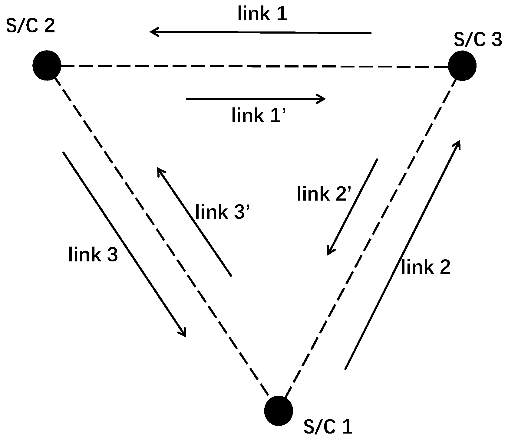
where each $y_{ij}$ represents a single-arm measurement taken from S/C i to S/C j, and the semicolon notation $y_{ij;k\dots }$ denotes that the measurement is further delayed by the light travel times along the specified sequence of links $k,\cdots$. A prime on a link index indicates that the laser travels in the opposite direction along that arm (e.g., $y_{21;2^{\prime }2}$ represents the single-arm measurement taken from S/C 2 to S/C 1, labeled at time $t-t_{13}-t_{31}$, where $t_{13}$ is the light travel time along the link 2, and $t_{31}$ is the light travel time along the link $2^{\prime }$, i.e., the same arm as link 2 but in the opposite direction); see Figure 1 for the labeling convention. The Y and Z combinations are constructed analogously by cyclic permutation of S/C indices: $1\to 2\to 3\to 1$ and $1\to 3\to 2\to 1$, respectively.

A second-generation TDI, denoted as TDI 2.0, of Michelson-type X combination centered on S/C 1 takes the form:

$$X_2\left(t\right)=\begin{array}{c}{X}_1\left(t\right)\hfill \\ +(y_{21;2^{\prime }{233}^{\prime }}+y_{12;2^{\prime }{233}^{\prime }3}+y_{31;2^{\prime }{233}^{\prime }{33}^{\prime }}+y_{13;2^{\prime }{233}^{\prime }{33}^{\prime }{2}^{\prime }})\hfill \\ -(y_{31;{33}^{\prime }{2}^{\prime }2}+y_{13;{33}^{\prime }{2}^{\prime }{22}^{\prime }}+y_{21;{33}^{\prime }{2}^{\prime }{22}^{\prime }2}+y_{12;{33}^{\prime }{2}^{\prime }{22}^{\prime }23}),\hfill \end{array}$$

(9)

with analogous constructions for the Y and Z combinations obtained via cyclic permutation of S/C indices. TDI 2.0 extends the delay structure, along with the inclusion of effects such as S/C orbital motion and time-dependent light travel times. These extensions are necessary to suppress laser-frequency noise below the level of the gravitational wave signal under realistic mission configurations.

The instrumental noise in the X, Y, and Z combinations is correlated due to their shared optical paths. To obtain statistically independent observables, these combinations are linearly transformed into the A, E, and T basis:

$$\begin{array}{cc}\hfill & A={\displaystyle \frac{1}{\sqrt{2}}}(Z-X),\hfill \\ \hfill & E={\displaystyle \frac{1}{\sqrt{6}}}(X-2Y+Z),\hfill \\ \hfill & T={\displaystyle \frac{1}{\sqrt{3}}}(X+Y+Z),\hfill \end{array}$$

(10)

in which the instrumental noise becomes uncorrelated. The A and E combinations are typically used for GW analysis, while T can serve as a noise-monitoring channel.

2.4. Taiji Data Challenge

The study in this paper uses the GB dataset from the original TDC, which provides simulated TDI 2.0 data generated using lisa-on-gpu code [65] with a GB parameter catalog. This catalog, initially provided in LDC1a, lists approximately 30 million GB sources, each specified by eight waveform parameters, collectively denoted by $\theta =\{f,\dot{f},\lambda ,\beta ,\mathcal{A},\iota ,\psi ,{\varphi }_0\}$. For further discussion of the GB population in the data, see relevant sections in P1 and P2. In the rest of the paper, we use the terms TDC and LDC for the GB-only datasets, and use LDC exclusively as shorthand for LDC1a, since other rounds such as LDC2a are not considered.

The data is provided in the form of TDI 2.0 in $AET$ combinations, covering an observation duration of $T_{\mathrm{obs}}=2\mathrm{yr}$ with a sampling interval of 10 s. It includes only GB signals and stationary Gaussian instrumental noise for simplicity. The noise is simulated directly in $AET$ combinations following the analytical noise power spectral densities (PSDs). The TDC data further includes a second time derivative of frequency, computed in the waveform model as $\ddot{f}=\frac{11}{3}{\dot{f}}^2/f$. The S/C orbits are modeled analytically as Keplerian, and light travel times are computed with corrections for S/C velocity, acceleration, and other relativistic effects to ensure accurate timing across links.

3. Overview of GBSIEVER

The GBSIEVER pipeline is designed to iteratively identify and subtract individual GB signals from GW data. The core algorithmic structure and data-processing framework are essentially those established in our earlier work. In contrast to the MATLAB-based GBSIEVER-M introduced in P1 and its subsequent extension to multi-detector networks in P2—both of which targeted TDI 1.0—this study presents two main updates. First, the pipeline is extended to support TDI 2.0, Second, it is fully re-implemented in a high-performance C-based version, GBSIEVER-C, enabling efficient, large-scale analyses. Due to the limited availability of robust simulated datasets for TDI 2.0, our current analysis is focused solely on single-detector TDI 2.0 data provided by TDC, nonetheless, the pipeline remains compatible with multi-detector network analyses.

We begin (Section 3.1) by briefly revisiting the single-source identification and parameter-estimation framework central to the iterative subtraction process, highlighting its straightforward extension from first- to second-generation TDI. Subsequently (Section 3.2), we succinctly summarize the various methodological components and data-processing steps employed, noting explicitly that the algorithmic choices and parameter settings remain identical to those detailed in P1.

3.1. Single-Source Estimation

The single-source identification and parameter estimation are fundamental within each iteration of the GBSIEVER pipeline. At every iteration, we assume the residual data contain exactly one dominant GB signal and employ MLE method to determine its parameters. The estimated signal is subsequently subtracted from the data to form a new residual, upon which the process repeats until predefined stopping criteria are reached.

To construct clean TDI 2.0 data, it is essential to accurately model the S/C orbital motion and the associated variations in light travel times, as these effects are required for canceling laser-frequency noise. In TDC, although laser noise is not simulated, the GB response signals do incorporate these effects, making accurate simulation of TDI 2.0 response to GBs computational expensive. Moreover, since MLE requires the TDI response to be repeatedly re-evaluated for different parameter sets, the computational cost is further increased.

To mitigate this cost, we adopt a simplified analytical model for the TDI 2.0 response [58], derived under certain well-justified approximations. In particular, the low-frequency nature of GW signals relative to the inverse arm-crossing time allows us to assume equal arm lengths and static S/C configurations. These approximations yield a highly efficient linear representation of the TDI 2.0 response at a given time t:

$${\overline{s}}^{\mathcal{I}}(t;\theta )=\sum _{i=1}^4{a}_i{X}_i^{\mathcal{I}}(t;\kappa ),$$

(11)

where $\mathcal{I}$ denotes a specific TDI combination (e.g., the Michelson-type X, Y, Z, or their recombinations A, E, T as defined in Equation (10)). We define $\overline{a}=(a_1,a_2,a_3,a_4)\in {\mathbb{R}}^4$ as a set of coefficients that re-parameterize the original astrophysical parameters $\{\mathcal{A},\iota ,\psi ,{\varphi }_0\}$; these are referred to as extrinsic parameters, as they can be estimated analytically. In contrast, $\kappa =\{f,\dot{f},\lambda ,\beta \}$ denotes the intrinsic parameters, which must be determined numerically. The functions $X_i^{\mathcal{I}}(t;\kappa )$ are template waveforms that depend only on intrinsic parameters. The full expressions of these waveforms, along with the mapping from original astrophysical parameters to $\overline{a}$, are provided in Appendix A. The TDI 1.0 response used in P1 and P2 follows the same overall structure, with only slight differences in the form of the $X_i^{\mathcal{I}}$ functions.

The accuracy of this modeling approach is numerically demonstrated in Figure 2, which compares TDI 2.0 signals generated using Equation (11) against the full TDI 2.0 data provided by TDC. For this comparison, we include all GB sources from the TDC catalog, but apply a frequency-domain filter to remove components above $15\mathrm{mHz}$—a region containing 18 high-frequency sources, most of which exhibit large second time derivative of frequency $\ddot{f}$. Since this analytical model currently does not account for $\ddot{f}$ effects, these sources are excluded to ensure a fair comparison. The negligible difference observed confirms the validity and effectiveness of this response model across the relevant frequency range.

Furthermore, this linear form allows the extrinsic parameters $\overline{a}$ to be analytically estimated from the likelihood expression, reducing the MLE problem to a numerical optimization over only the intrinsic parameters $\kappa$:

$$\widehat{\kappa }=\underset{\kappa }{\mathrm{argmax}}\mathcal{F}\left(\kappa \right).$$

(12)

Here, $\widehat{\kappa }$ denotes the estimates of $\kappa$ (the same hat notation will be used for other parameters as well), and the symbol written underneath argmax specifies the variables over which the maximization is performed. Once $\widehat{\kappa }$ is determined, the corresponding extrinsic parameters can be recovered from the data, yielding a complete estimate of the source parameters $\widehat{\theta }=\{\widehat{a},\widehat{\kappa }\}$. The function $\mathcal{F}\left(\kappa \right)$ in the above expression is known as $\mathcal{F}$-statistic, which plays a central role in governing the pipeline’s performance. Detailed derivations are available in P1 for the single-detector case and in P2 for the multi-detector extension.

In this pipeline, $\mathcal{F}\left(\kappa \right)$ serves as the fitness function in a PSO algorithm—a global optimization method that efficiently explores the parameter space, with higher fitness values indicating better parameter fits. In GBSIEVER, we adopt the lbest PSO, a widely used variant of PSO known for robust convergence properties [66]. In this scheme, each particle acts as a search agent navigating the parameter space. During every PSO step, each particle evaluates the fitness function, making this process naturally parallelizable across particles. In addition, a Best-of-N PSO runs approach is applied: in each iteration of source identification and subtraction, N independent PSO searches are performed, and only the best-performing result is retained. This approach significantly improves the probability of global convergence—if a single PSO run fails with probability p, then N independent runs succeed with probability $1-p^N$—while maintaining reasonable computational cost. Like the particle-level evaluations, this Best-of-N strategy is also naturally parallelizable. In this paper, we set the number of independent PSO runs to 6, with each run using 40 particles and 2000 PSO steps.

3.2. Key Methods and Parameter Settings

The methods employed in GBSIEVER are detailed comprehensively in P1. Here, we summarize key implementation aspects.

Frequency-band segmentation: Because each GB signal occupies only a narrow range in frequency space, we divide the full TDI dataset into overlapping frequency bands of width 0.02 mHz, covering the search range of $[0.1,15]$ mHz. This segmentation localizes the analysis, allows for parallel execution across bands, and substantially reduces the effective number of data points per band. However, segmentation introduces artificial boundaries that must be carefully handled to avoid spurious effects.

Edge-effect mitigation: Without proper treatment, signal components near the edges of each frequency band can lead to systematic parameter-estimation errors and the repeated detection of spurious sources. To address this, we apply a Tukey window to each frequency band. The window consists of a flat central region covering 75% of the band and smoothly tapering edges on either side. In addition, adjacent bands are overlapped by 50%. Identified sources are those only located within the central 0.01 mHz, referred to as the acceptance zone, thereby ensuring full frequency coverage and robustness against boundary artifacts.

White noise approximation: Within each narrow frequency band, the noise PSD can be treated as constant. Since the $\mathcal{F}$-statistic involves the noise-weighted inner product defined in the frequency domain, this approximation allows the PSD term to be factored out. Consequently, Parseval’s theorem can be applied to evaluate the inner product in the time domain. This eliminates the need for repeated Fourier transforms and reduces computational overhead.

Undersampling: Since the data have already been bandpass-filtered and the template waveforms used in parameter estimation are narrowband, we can apply undersampling—a special form of downsampling that allows the sampling rate to fall below the Nyquist limit without loss of information [67]. This reduces the number of data points involved in both template generation and inner product evaluation in $\mathcal{F}$-statistic. The reduction factor of this undersampling rate, compared to the standard downsampling rate associated with the Nyquist frequency, varies approximately linearly with frequency across different bands. For reference, it is around 250 at 5 mHz and 500 at 10 mHz. This reduction is critical, as $\mathcal{F}$-statistic must be evaluated repeatedly during the PSO process to explore the parameter space.

Termination criteria: Each frequency band is iteratively processed until one of two stopping conditions is met. First, if the SNR (defined as in P1) of the estimated sources falls below a fixed threshold of 7 for five consecutive iterations, the band is considered exhausted of detectable sources. Second, an upper limit of 200 iterations is imposed to prevent unnecessarily long runtimes in high-density bands. Both criteria are consistent with those used in P1. While in P2, a larger iteration cap was adopted to accommodate the higher number of resolvable sources expected in multi-detector network analyses.

Block-wise cross-validation: Below 4 mHz, where signal density is high, we perform two independent searches per frequency band—primary (narrow $\dot{f}$ search range) and secondary (wide $\dot{f}$ search range). Correlation measures ($R_{\mathrm{ee}}$) between identified sources in these two searches are computed. The $R_{\mathrm{ee}}$ value ranges from $-1$ to 1, with values close to 1 indicating high agreement between two candidate sources, values near 0 suggesting they are uncorrelated, and values near $-1$ representing strong anti-correlation, which is generally not expected in this context. To determine the final set of reported sources, we apply block-wise selection criteria to the identified sources described above, by requiring their $R_{\mathrm{ee}}$ values to be greater than the corresponding thresholds. Specifically, the frequency–SNR space is partitioned into several coarse blocks that reflect different levels of foreground contamination, and each block is assigned a fixed $R_{\mathrm{ee}}$ threshold accordingly. This selection procedure effectively reduces false positives arising from foreground confusion noise. The choice of blocks and $R_{\mathrm{ee}}$ cutoff values is relatively flexible and reflects a practical balance between the reliability and completeness of the reported sources.

4. Implementation Details and Optimizations

This section outlines the computational design and implementation of the current C-based pipeline, GBSIEVER-C, which represents a substantial re-engineering of an earlier MATLAB prototype. The discussion is organized around four key themes: (i) a hierarchical three-level parallel architecture (Section 4.1); (ii) the use of Cholesky decomposition to accelerate and stabilize evaluations of the $\mathcal{F}$-statistic (Section 4.2); (iii) a suite of micro-optimizations addressing thread-level performance bottlenecks (Section 4.3); and (iv) the computational cost, expressed in core-hours, measured on two (high-performance computing) HPC platforms (Section 4.4). Unless otherwise specified, all discussions pertain to the search stage (i.e., the stage for obtaining the identified sources) of the GBSIEVER-C pipeline; other stages, such as cross-validation and result evaluation, are relatively lightweight and are therefore omitted here.

To support the architecture and optimizations described above, our C implementation relies on several well-established third-party libraries that provide numerically robust functions, efficient I/O, and portable parallel primitives:

• The GNU Scientific Library (GSL) [68] is a widely used numerical toolkit; in our code, we depend only on its reliable random-number generators, a choice that leaves the rest of the code free to migrate later to GPU kernels with minimal effort.
• Open Multi-Processing (OpenMP) [69] introduces shared-memory parallelism via simple compiler directives, allowing multiple CPU cores to collaborate on the same workload with little change to the original serial code.
• Fastest Fourier Transform in the West 3 (FFTW3) [70] delivers highly efficient discrete Fourier transforms for many problem sizes and processor types, accelerating every frequency-domain step in the pipeline.
• Hierarchical Data Format version 5 (HDF5) [71] records intermediate results and final outputs in a portable, self-describing binary file structure that supports chunked layout and optional compression, ensuring efficient I/O on large datasets.
• Libfyaml [72] is a C library for reading configuration files written in YAML Ain’t Markup Language (YAML) [73], a plain-text format designed to be both human-readable and machine-friendly; using YAML keeps run-time options easy to edit without recompiling.

4.1. Multi-Level Parallel Architecture

The search stage of GBSIEVER-C employs a three-level parallel architecture (see Figure 3) for efficiently analyzing TDI data. At the outermost level, the full frequency range is partitioned into sub-bands, each completed by a standalone C executable task with corresponding frequency index and YAML file paths as input arguments. These arguments are organized into a shared task pool accessible by all compute nodes. Each node uses a dispatching shell script to sequentially fetch and execute tasks from this pool one by one. A synchronization lock is used to ensure that no two nodes process the same task simultaneously. This dynamic allocation balances the workload by letting idle nodes pick up remaining tasks as soon as they finish. The task-pool mechanism here is required in practice, as the number of compute nodes that can be simultaneously allocated to a user is typically smaller than the number of sub-bands.

Within each frequency band, unlike the previous MATLAB version where the language supports only single-level parallelism, GBSIEVER-C adopts a nested parallel strategy implementation using OpenMP. The outer OpenMP level corresponds to the Best-of-N PSO runs approach described in Section 3.1, assigning each run to a separate thread. The inner OpenMP level operates within each PSO run, evaluating the fitness values at different particle positions in parallel. A round-robin scheduling strategy is used to assign an approximately equal number of PSO runs or particles to OpenMP threads. While the let-them-fly boundary condition we applied in PSO allows particles to exit the predefined search domain, not all particles require fitness evaluation in every PSO step. This suggests room for further efficiency gains by dynamically adjusting thread assignments based on actual evaluation needs.

For all executables (tasks), the number of OpenMP threads used in the outer and inner loops is specified in a shared configuration file, along with other settings such as the parameter search range, number of independent PSO runs, and detailed PSO settings. These thread counts are tuned to match the hardware of the compute nodes, which are typically equipped with an identical number of CPU cores. In the context of OpenMP, we carefully manage the allocation of shared and private variables to balance memory usage and computational efficiency. Variables that do not require thread-local copies—such as precomputed S/C orbits or TDI data used in the fitness function ($\mathcal{F}$-statistic) evaluations—are declared as shared variables to avoid unnecessary duplication. In contrast, variables tied to per-thread computations, including particle positions or temporary buffers, are kept private to ensure thread safety. This strategy effectively reduces memory overhead while preventing redundant computation.

4.2. Cholesky Decomposition for Rapid $\mathcal{F}$-Statistic Evaluation

Since the $\mathcal{F}$-statistic is used as the fitness function inside PSO, it must be evaluated repeatedly. In this paper, each iteration of GBSIEVER is configured with 6 independent PSO runs, each evolving 40 particles for 2000 PSO steps. This already triggers $6\times 40\times 2000=4.8\times {10}^5$ calls to $\mathcal{F}$-statistic; many such iterations are executed for every frequency band, so the cumulative count soon reaches the multi-million scale. Each $\mathcal{F}$-statistic evaluation reduces the quadratic form

$$\mathcal{F}\left(\kappa \right)={\mathbf{U}}^T{\mathbf{W}}^{-1}\mathbf{U},$$

(13)

where $\mathbf{W}$ is typically a symmetric 4-by-4 positive-definite matrix and $\mathbf{U}$ is 4 dimensional column vector. Forming the explicit inverse ${\mathbf{W}}^{-1}$ would be needlessly expensive and, more importantly, would magnify rounding errors. Instead, our C code applies the Cholesky decomposition [74,75], which factorizes $\mathbf{W}$ into the product of a lower triangular matrix and its transpose, $\mathbf{W}=\mathbf{L}{\mathbf{L}}^T$. We then solve the two triangular systems $\mathbf{L}\mathbf{y}=\mathbf{U}$ (forward substitution) and ${\mathbf{L}}^T\mathbf{x}=\mathbf{y}$ (backward substitution); the desired scalar follows immediately as $\mathcal{F}={\mathbf{U}}^T\mathbf{x}$. Because triangular solves scale much better than a full inversion and avoids ill-conditioning, this strategy is both faster and more numerically robust. equivalently and more efficiently, we could have obtained it by ${\mathbf{y}}^T\mathbf{y}$ directly, which saves the second triangular solve. But triangular solves are only a small fraction of the total runtime, so the net speedup of changing to ${\mathbf{y}}^T\mathbf{y}$ is minor; the key benefit, in either form, is to avoid forming the inverse of $\mathbf{W}$ explicitly. Our implementation originally followed the two-solve scheme, and all results in this paper are based on that version. We will adopt the single-solve form in future work.

It is also worth noting that MATLAB’s backslash operator (\) also solves linear systems without explicitly computing matrix inverses. MATLAB selects an appropriate solver based on the numerical properties of the matrix encountered at runtime. If the matrix is detected to be symmetric and numerically positive definite, MATLAB typically employs Cholesky decomposition internally; otherwise, it switches to alternative numerical methods suited to the detected matrix characteristics.

4.3. Additional Performance Optimizations

Our C implementation employs several additional performance optimizations beyond parallel execution and Cholesky decomposition. First, we make use of the automatic optimization features provided by standard C compilers, particularly the -O3 optimization flag—the most aggressive among the standard optimization levels in GCC and Intel compilers—which enhances instruction scheduling, loop unrolling, vectorization, and aggressive function inlining to improve overall execution speed.

Furthermore, memory access patterns were carefully optimized, particularly for computationally intensive operations such as vector–matrix and matrix–matrix multiplications. With the -O3 optimization flag enabled, we benchmarked typical matrix dimensions under different memory layouts (row-major vs. column-major) and operation orders. These tests informed our choice of data layout and computation order to improve memory locality, ensuring that jointly accessed elements are stored contiguously in memory. This significantly reduces memory access overhead and enhances overall performance.

Additionally, redundant computations were minimized by precomputing and reusing intermediate results. In particular, trigonometric functions such as sin and cos—which are significantly more expensive than basic arithmetic, since these transcendental functions are typically computed via polynomial approximations and iterative algorithms—were computed once per iteration where possible and cached. Similar reuse strategies were applied to other costly operations, such as template functions and S/C orbit calculations, to reduce redundant evaluations in performance-critical loops.

4.4. Measured Core-Hour Performance

To quantify the computational cost of the optimized C implementation, we measured the total core-hours consumed during the primary and secondary searches on two HPC clusters. These measurements pertain to the search stage of GBSIEVER-C. Here, a core-hour is defined as the product of the wall time and the number of CPU cores allocated to each parallel task which corresponds to each frequency band. The benchmarked workload corresponds to the analysis of TDC data based on TDI 2.0, which forms the primary focus of this study.

The first system is the Lonestar6 cluster at the Texas Advanced Computing Center (TACC), where each compute node is equipped with two AMD EPYC 7763 processors, providing a total of 128 physical cores and 256 GB of DDR4 memory per node. In our tests, each task was allocated 128 CPU cores, with OpenMP configured to execute 6 PSO runs concurrently, each employing 20 threads to compute fitness values for 40 PSO particles in parallel (labeled as 6 × 20 threads, totaling 120). The total core-hours recorded were 12,246 for the primary search and 10,354 for the secondary search.

The second system is the LSSC-IV cluster at the Institute of Mathematics, Chinese Academy of Sciences (CAS), hereafter referred to as the CAS cluster. Each compute node is equipped with two 18-core Intel Xeon Gold 6140 CPUs at 2.30 GHz, providing 36 physical cores per node. We tested two OpenMP configurations: 6 × 14 and 6 × 8. Both configurations yielded similar results, with the 6 × 14 setting consuming 16,968 core-hours for the primary search and 13,620 core-hours for the secondary search, while the 6 × 8 configuration differed by less than 50 core-hours in each case. This negligible difference suggests that the total core-hour usage on this cluster is relatively insensitive to the precise choice of thread configuration, provided that the OpenMP configuration is reasonably chosen.

While the total computational workload remained unchanged across clusters, the observed reduction in core-hours on TACC may be attributed not only to hardware-level factors such as cache and memory bandwidth, but also to a more favorable match between the thread configuration (6 × 20) and the number of particles per PSO run (40). This alignment leads to improved load distribution and better utilization of computational resources, contributing to lower wall time and hence reduced core-hour consumption.

On the TACC cluster, the maximum wall time per task (either primary or secondary search) is about 18 min. This means that if all tasks are executed in parallel, a full primary or secondary search completes within 18 min. In contrast, the corresponding wall time on the CAS cluster is approximately 75 min, primarily due to the lower number of cores per node (36 cores on CAS versus 128 on TACC).

Although a fully parallelized MATLAB version was not available for benchmarking due to its lack of support for multi-level parallelism, we conducted a preliminary comparison between GBSIEVER-M and GBSIEVER-C on a personal workstation. Under a simplified configuration using only outer-level OpenMP parallelism (Best-of-N PSO runs with $N=6$), the C implementation completed in approximately 1/5 the time required by MATLAB. This ratio is only a rough estimate, as runtime is sensitive to a variety of factors—including memory usage, CPU scheduling, and background processes—and should not be interpreted as a precise speedup. Furthermore, further scaling on the personal machine was constrained by its limited core count, highlighting the importance of running the GBSIEVER-M on high-core-count clusters to fully exploit the performance improvement benefit from the C implementation.

Future Architectural Directions

The use of a shell-based workflow management is a legacy of the Matlab code, since that was the only option. In the future, the outermost level of parallelism could be further automated and optimized using Message-Passing Interface (MPI) [76]. Compared to shell scripts, an MPI-based architecture would enable more dynamic task distribution, better load balancing, and tighter synchronization across computed nodes. For example, a more unified parallel strategy could flatten the current multi-level design, allowing fitness evaluations from different PSO runs or frequency bands to proceed concurrently. This would improve resource utilization by decoupling the fixed association between compute nodes and frequency bands.

Additionally, OpenMP-based GPU offloading could be explored in future implementations to accelerate the most compute-intensive parts of the pipeline, such as inner-product operations within the fitness evaluation steps. These enhancements would allow GBSIEVER-C to better scale on modern heterogeneous HPC platforms.

5. Results

This section presents a comprehensive evaluation of the GBSIEVER-C pipeline across several key performance aspects. We begin by examining its resolution performance on the TDC dataset (Section 5.1), including tests of platform-level reproducibility and sensitivity to the stochastic elements of PSO. We then examine subtraction residuals (Section 5.2) and parameter estimation accuracy (Section 5.3), both essential for validating the pipeline’s ability to isolate and characterize individual GB sources. Finally, using GBSIEVER-C, we reproduce key results from the prior MATLAB-based studies on the LDC (P1) and LISA–Taiji network (P2) datasets (Section 5.4), demonstrating consistency across computing platforms and random number configurations.

As noted in Section 3, reported sources refer to the final subset selected from identified candidates after applying specific $R_{\mathrm{ee}}$ cuts. To better present the results in this section, we further define confirmed sources as those reported entries that successfully match injected (true) sources based on a prescribed association metric. The detection rate is then defined as the ratio of confirmed to reported sources.

5.1. Source Resolution Performance

To evaluate the resolution performance of GBSIEVER-C on the TDC dataset, we compute the number of reported and confirmed sources in each frequency–SNR block under the so-called Main selection settings used in our previous analyses (P1 and P2). The results, summarized in

Table 1. Resolution performance of GBSIEVER-C on the TDC GB dataset under the Main selection settings. The data are divided into five contiguous frequency–SNR blocks, each with a potentially different $R_{\mathrm{ee}}$ threshold depending on the foreground noise level. For $f\le 4$ mHz, cross-validation is performed using two $\dot{f}$ search ranges: $[-{10}^{-16},{10}^{-15}]{\mathrm{Hz}}^2$ for the primary search and $[-{10}^{-14},{10}^{-13}]{\mathrm{Hz}}^2$ for the secondary search. For $f\in [4,15]$ mHz, only the primary search is performed with the same range of $[-{10}^{-14},{10}^{-13}]{\mathrm{Hz}}^2$, and a value of $R_{\mathrm{ee}}=-1$ in this block indicates that no $R_{\mathrm{ee}}$ threshold was applied. All identified sources shown are obtained from the CAS cluster using random number sequences a.

	$\mathit{\nu }$ mHz	SNR	$\mathit{\nu }$ mHz	SNR	$\mathit{\nu }$ mHz	SNR	$\mathit{\nu }$ mHz	SNR	$\mathit{\nu }$ mHz	SNR
	$[\mathbf{0},\mathbf{3}]$	$[\mathbf{0},\mathbf{25}]$	$[\mathbf{0},\mathbf{3}]$	$[\mathbf{25},\infty ]$	$[\mathbf{3},\mathbf{4}]$	$[\mathbf{0},\mathbf{20}]$	$[\mathbf{3},\mathbf{4}]$	$[\mathbf{20},\infty ]$	$[\mathbf{4},\mathbf{15}]$	$[\mathbf{10},\infty ]$
$R_{\mathrm{ee}}$	$0.9$		$0.5$		$0.9$		$0.5$		$-1$
Identified	24,810		3582		3748		2799		5010
Reported	2040		3398		1219		2729		5010
Confirmed	1233		2880		948		2424		4496
Detection rate	$60.44\%$		$84.76\%$		$77.77\%$		$88.82\%$		$89.74\%$
Lowest SNR (confirmed)	$7.60$				$7.29$				$10.02$
Total reported	14,396
Total confirmed	11,981
Detection rate	$83.23\%$

, reflect the pipeline’s behavior across varying foreground conditions. For $f>4$ mHz, where the foreground becomes negligible, cross-validation is not applied and the $R_{\mathrm{ee}}$ threshold is formally set to $-1$.

We conducted additional analyses to assess both the cross-platform reproducibility and the influence of randomness on the pipeline results. The results summarized earlier (Table 1) correspond to the CAS cluster run using a specific set of random number sequences—referred to as sequences a—generated by assigning different seeds to corresponding PSO runs. Unless otherwise noted, subsequent discussions of the TDC results refer to this CAS run using sequences a under the Main selection settings. The corresponding results from the TACC cluster using the same sequences (a), and from an additional CAS run using different sequences (b), are provided in Appendix B (

Table A1. Resolution performance of GBSIEVER-C on the TDC GB dataset under the Main selection settings. The data are divided into five contiguous frequency–SNR blocks, each with a potentially different $R_{\mathrm{ee}}$ threshold depending on the foreground noise level. For $f\le 4$ mHz, cross-validation is performed using two $\dot{f}$ search ranges: $[-{10}^{-16},{10}^{-15}]{\mathrm{Hz}}^2$ for the primary search and $[-{10}^{-14},{10}^{-13}]{\mathrm{Hz}}^2$ for the secondary search. For $f\in [4,15]$ mHz, only the primary search is performed with the same range of $[-{10}^{-14},{10}^{-13}]{\mathrm{Hz}}^2$, and a value of $R_{\mathrm{ee}}=-1$ in this block indicates that no $R_{\mathrm{ee}}$ threshold was applied. All identified sources shown are obtained from the TACC cluster using random number sequences a.

	$\mathit{\nu }$ mHz	SNR	$\mathit{\nu }$ mHz	SNR	$\mathit{\nu }$ mHz	SNR	$\mathit{\nu }$ mHz	SNR	$\mathit{\nu }$ mHz	SNR
	$[\mathbf{0},\mathbf{3}]$	$[\mathbf{0},\mathbf{25}]$	$[\mathbf{0},\mathbf{3}]$	$[\mathbf{25},\infty ]$	$[\mathbf{3},\mathbf{4}]$	$[\mathbf{0},\mathbf{20}]$	$[\mathbf{3},\mathbf{4}]$	$[\mathbf{20},\infty ]$	$[\mathbf{4},\mathbf{15}]$	$[\mathbf{10},\infty ]$
$R_{\mathrm{ee}}$	$0.9$		$0.5$		$0.9$		$0.5$		$-1$
Identified	24,813		3580		3733		2800		4995
Reported	2046		3402		1231		2726		4995
Confirmed	1244		2885		974		2420		4487
Detection rate	$60.80\%$		$84.80\%$		$79.12\%$		$88.78\%$		$89.83\%$
Lowest SNR (confirmed)	$7.60$				$7.44$				$10.02$
Total reported	14,400
Total confirmed	12,010
Detection rate	$83.40\%$

and 

Table A2. Resolution performance of GBSIEVER-C on the TDC GB dataset under the Main selection settings. The data are divided into five contiguous frequency–SNR blocks, each with a potentially different $R_{\mathrm{ee}}$ threshold depending on the foreground noise level. For $f\le 4$ mHz, cross-validation is performed using two $\dot{f}$ search ranges: $[-{10}^{-16},{10}^{-15}]{\mathrm{Hz}}^2$ for the primary search and $[-{10}^{-14},{10}^{-13}]{\mathrm{Hz}}^2$ for the secondary search. For $f\in [4,15]$ mHz, only the primary search is performed with the same range of $[-{10}^{-14},{10}^{-13}]{\mathrm{Hz}}^2$, and a value of $R_{\mathrm{ee}}=-1$ in this block indicates that no $R_{\mathrm{ee}}$ threshold was applied. All identified sources shown are obtained from the CAS cluster using random number sequences b.

	$\mathit{\nu }$ mHz	SNR	$\mathit{\nu }$ mHz	SNR	$\mathit{\nu }$ mHz	SNR	$\mathit{\nu }$ mHz	SNR	$\mathit{\nu }$ mHz	SNR
	$[\mathbf{0},\mathbf{3}]$	$[\mathbf{0},\mathbf{25}]$	$[\mathbf{0},\mathbf{3}]$	$[\mathbf{25},\infty ]$	$[\mathbf{3},\mathbf{4}]$	$[\mathbf{0},\mathbf{20}]$	$[\mathbf{3},\mathbf{4}]$	$[\mathbf{20},\infty ]$	$[\mathbf{4},\mathbf{15}]$	$[\mathbf{10},\infty ]$
$R_{\mathrm{ee}}$	$0.9$		$0.5$		$0.9$		$0.5$		$-1$
Identified	24,841		3579		3740		2799		4990
Reported	2189		3421		1301		2740		4990
Confirmed	1316		2897		1029		2431		4523
Detection rate	$60.12\%$		$84.68\%$		$79.09\%$		$88.72\%$		$90.64\%$
Lowest SNR (confirmed)	$7.34$				$7.29$				$10.08$
Total reported	14,641
Total confirmed	12,196
Detection rate	$83.30\%$

, respectively). When comparing CAS and TACC results under the same random number sequences, the number of identified and reported sources each differs by fewer than 30 per block, confirming the numerical portability of the C implementation across hardware platforms. These small discrepancies are attributable to hardware or runtime-level effects. In contrast, using different sequences (CAS with sequences b) leads to modest variations in the reported and confirmed source counts, demonstrating the extent to which algorithmic randomness can influence resolution performance.

As noted in Section 2, the TDC data were generated using a GB source catalog identical to that of LDC. This makes it reasonable to compare our TDC results to earlier LDC analyses (unless otherwise stated, referring to the single-detector results in P2, which reproduce those of P1), where the same algorithm and selection criteria were applied to TDI 1.0 data. Compared to the LDC LISA detector results, the detection rate decreases slightly, from $84.79\%$ to $83.23\%$. However, the TDC analysis yields a substantial increase in both reported and confirmed source counts: the total number of reported sources rises from $12,251$ to $14,396$, and confirmed sources from $10,388$ to $11,981$. These gains reflect the improved SNR in the TDC dataset, driven by differences in detector arm length and noise modeling as discussed below.

The SNR of a given source can differ across datasets, depending on factors such as the noise PSD, the TDI generation used, and the total observation time. In our case, the observation time is the same for both datasets. Moreover, in principle, if the noise simulation and related noise parameters are consistent across both datasets, the transition from first- to second-generation TDI should not affect the SNR, as both the TDI signal magnitude and the noise PSD are transitioned in a way that ideally cancels out in the SNR calculation. The only systematic factor expected to cause a net difference is the detector arm length, which contributes a multiplicative factor in SNR equal to the arm length ratio (=1.2). However, the TDC dataset uses a different noise simulation and configuration from the LDC dataset, leading to a further change in SNR. For reference, the average SNR ratios (TDC/LDC), computed over all true sources in the catalog, are $1.34$ in the low-frequency band ($f<3$ mHz), $1.59$ in the middle band ($3\le f<4$ mHz), and $1.98$ in the high-frequency band ($f\ge 4$ mHz).

To better illustrate the sensitivity of our results to the SNR threshold, we also processed the data using a stricter cutoff—set to $1.2$ times the original value (see

Table 2. Resolution performance of GBSIEVER-C on the TDC GB dataset under the Strict selection settings. The data are divided into five contiguous frequency–SNR blocks, each with a potentially different $R_{\mathrm{ee}}$ threshold depending on the foreground noise level. Compared to the Main setting, the SNR cutoffs in each block are increased by a factor of 1.2: specifically, to 30 for $f<3$ mHz, to 24 for $f\in [3,4]$ mHz, and to 12 for $f\ge 4$ mHz. For $f\le 4$ mHz, cross-validation is performed using two $\dot{f}$ search ranges: $[-{10}^{-16},{10}^{-15}]{\mathrm{Hz}}^2$ for the primary search and $[-{10}^{-14},{10}^{-13}]{\mathrm{Hz}}^2$ for the secondary search. For $f\in [4,15]$ mHz, only the primary search is performed with the same range of $[-{10}^{-14},{10}^{-13}]{\mathrm{Hz}}^2$, and a value of $R_{\mathrm{ee}}=-1$ in this block indicates that no $R_{\mathrm{ee}}$ threshold was applied. All identified sources shown are obtained from the CAS cluster using random number sequences a.

	$\mathit{\nu }$ mHz	SNR	$\mathit{\nu }$ mHz	SNR	$\mathit{\nu }$ mHz	SNR	$\mathit{\nu }$ mHz	SNR	$\mathit{\nu }$ mHz	SNR
	$[\mathbf{0},\mathbf{3}]$	$[\mathbf{0},\mathbf{30}]$	$[\mathbf{0},\mathbf{3}]$	$[\mathbf{30},\infty ]$	$[\mathbf{3},\mathbf{4}]$	$[\mathbf{0},\mathbf{24}]$	$[\mathbf{3},\mathbf{4}]$	$[\mathbf{24},\infty ]$	$[\mathbf{4},\mathbf{15}]$	$[\mathbf{12},\infty ]$
$R_{\mathrm{ee}}$	$0.9$		$0.5$		$0.9$		$0.5$		$-1$
Identified	25,849		2543		4319		2228		4830
Reported	2757		2494		1680		2194		4830
Confirmed	1779		2231		1343		1983		4463
Detection rate	$64.53\%$		$89.46\%$		$79.94\%$		$90.38\%$		$92.40\%$
Lowest SNR (confirmed)	$7.60$				$7.29$				$12.00$
Total reported	13,955
Total confirmed	11,799
Detection rate	$84.55\%$

). This factor serves as a simplified approximation for the actual SNR scaling. When applying this more conservative threshold, the number of reported and confirmed sources decreased to $13,955$ and $11,799$, respectively. However, the overall detection rate improved from $83.23\%$ to $84.55\%$, reflecting a trade-off between completeness and reliability, as expected. Even under this stricter condition, the reported and confirmed source counts still exceed those in our earlier LDC analysis while the detection rate remains comparable ($84.55\%$ vs. $84.79\%$). This suggests that the gains observed under the Main selection in TDC results are not solely due to the inclusion of spurious sources, but also reflect a genuine improvement in detection performance.

The current $R_{\mathrm{ee}}$ thresholds are fixed across predefined frequency blocks and do not account for variations in data characteristics under different observational settings, such as mission duration or detector configuration. The design of these blocks and thresholds is also guided by theoretical expectations for the GB population. While this static scheme provides a consistent baseline, a more robust strategy would be to develop a self-adaptive, data-driven approach that can adjust block definitions and thresholds according to the properties of each dataset and the desired trade-off between search depth (i.e., the lowest recoverable SNR) and reliability.

5.2. Residuals

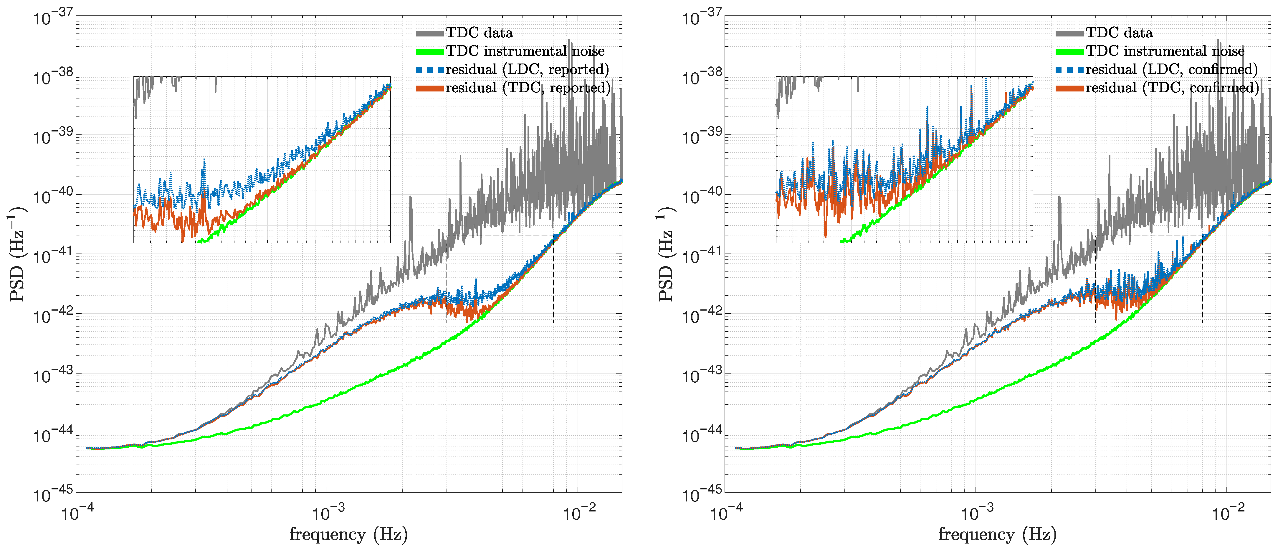
The effectiveness of GB signal subtraction can be assessed by examining the residual after subtracting the reported sources from the data. Figure 4 illustrates the residual after subtraction, using the TDI A combination, in both the Fourier amplitude (left) and PSD (right) panels. The right panel also includes the instrumental noise PSD estimated from TDC dataset. Ideally, if all GB signals were perfectly removed, the resulting residual would match the instrumental noise level. In reality, this is unattainable—particularly at frequencies below ∼4 mHz, where the high density of overlapping sources gives rise to a foreground noise component. Despite this challenge, a sufficiently accurate subtraction can still greatly reduce the overall residual level, which is essential for enabling the detection of other types of sources in future analyses.

Figure 5 illustrates the comparison between the TDC and LDC results. It compares the TDC residuals obtained by subtracting either the reported sources (left) or the confirmed sources (right), with the corresponding LDC residuals. Note that these LDC residuals here are obtained by subtracting, from the TDC data, the TDI 2.0 signals corresponding to the LDC-reported sources. Although the original LDC result is based on TDI 1.0 and LISA orbits, while the TDC dataset adopts TDI 2.0 and Taiji orbits, this projection allows for a meaningful comparison of the residuals under a unified framework.

The difference between the left and right panels in Figure 5 suggests that both the TDC and LDC analyses exhibit some degree of signal mis-subtraction. When only the confirmed sources are subtracted (right panel)—instead of all reported ones (left panel)—additional high-frequency spikes emerge in the residual. This implies that some spurious sources may have led to the removal of signal content that was not correctly recovered. This can occur, for example, when two nearby high-SNR sources are mistakenly modeled as one, or when amplitude mismatches lead to incomplete cancellation. These findings suggest that, although the residuals in the left panel appear to align closely with the instrumental noise level, they may still reflect imperfect or inaccurate signal removal. This motivates further improvement of GBSIEVER to incorporate global-fit algorithms that simultaneously fit multiple sources in cases of strong source overlap.

5.3. Parameter-Estimation Performance

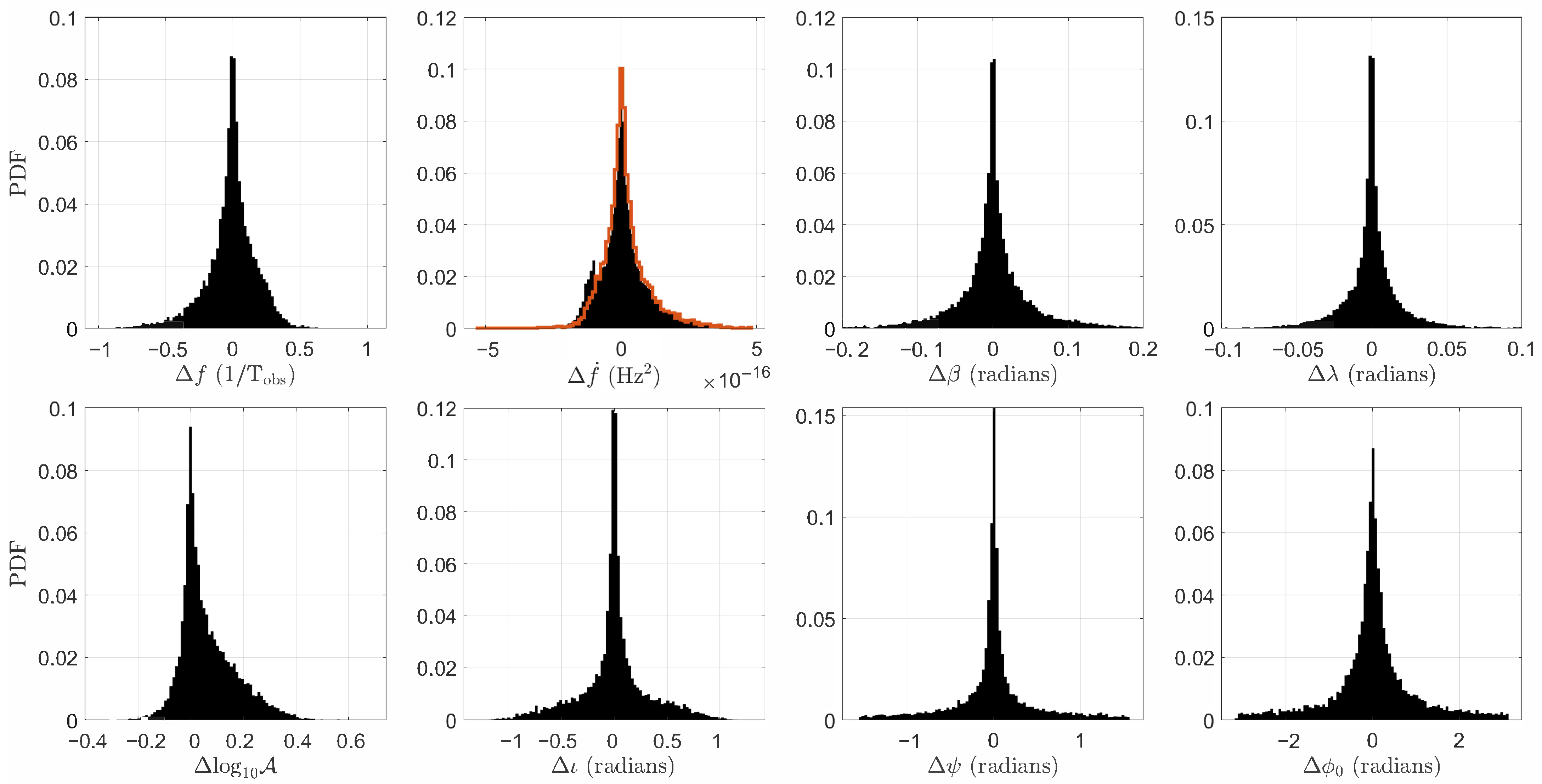
To evaluate the parameter-estimation performance of GBSIEVER-C on the TDC dataset, we compute the differences between the estimated values and the corresponding true values of all 8 waveform parameters—referred to as estimation errors—while accounting for and resolving parameter degeneracies. Figure 6 shows histograms of these errors for all confirmed sources. The distributions exhibit narrow peaks centered around zero, indicating that the parameter estimates are generally accurate and unbiased.

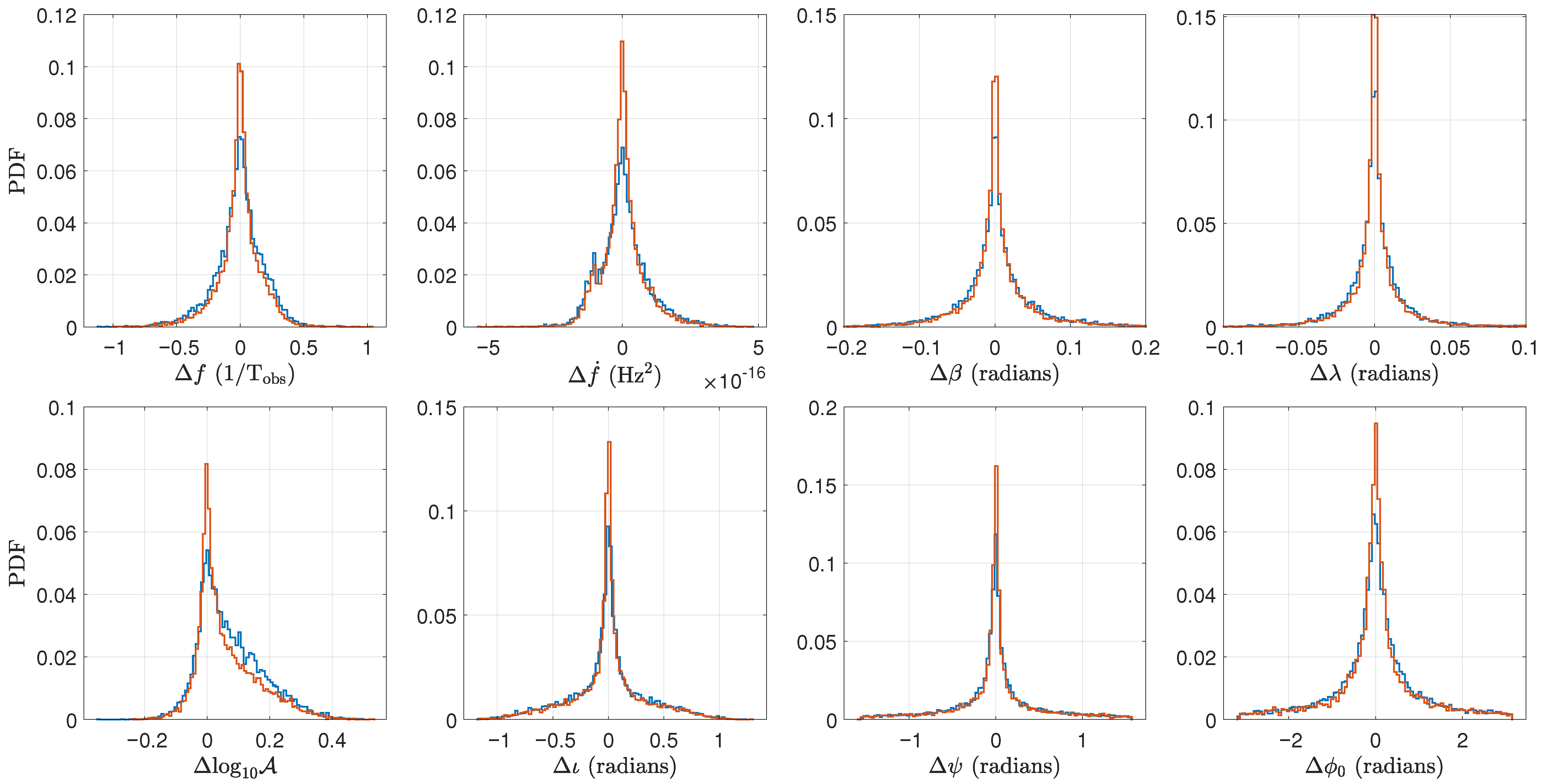
We further examine the subset of sources that are confirmed in both the TDC and LDC analyses. For these common sources, Figure 7 compares the distributions of estimation errors obtained from the TDC data (in red) and the LDC data (in blue). The red curves are generally narrower and more sharply peaked, suggesting that the TDC analysis tends to yield lower parameter-estimation errors for the same sources. This is consistent with the fact that these signals tend to have higher SNRs in the TDC dataset, due to differences in detector arm length and noise models.

Notably, the number of confirmed sources common to both the TDC and LDC analyses is 9673, compared to a total of $10,388$ confirmed sources in the LDC analysis. This indicates that a non-negligible fraction of LDC-confirmed sources were not recovered in the TDC results, despite the latter yielding a higher overall number of confirmed detections. For context, the number of common confirmed sources in the P2 analysis—comparing LISA-only (i.e., LDC) and LISA–Taiji network results—was higher ($10,287$), suggesting that the discrepancy observed here is more pronounced.

These findings point to a non-trivial relationship between which sources are detected and which ones are ultimately confirmed, particularly when comparing datasets that differ not only in noise characteristics but also in detector baselines, orbital configurations, and the generation of TDI employed. Understanding this relationship may reveal deeper insights into the limitations and strengths of different data sources, and how these factors influence the performance of the GBSIEVER pipeline in recovering GB signals. Further analysis, possibly involving detectability studies with injected signals, may help isolate the causes of such discrepancies and improve the robustness of confirmation strategies across datasets.

5.4. Consistency with Prior Results

To verify the consistency and correctness of the GBSIEVER-C implementation, we reproduced the analyses presented in P1 and P2. P1 focused on GBs in the LDC dataset, while P2 extended the study to a joint observation by the LISA–Taiji network, using the same LDC dataset for the LISA data and modeling the Taiji detector with the same arm length as LISA. In both cases, the original analyses were conducted using GBSIEVER-M, which is the MATLAB version of the pipeline. Here, we reprocess the same datasets using the C implementation on two independent computing platforms: the TACC and CAS clusters.

Table 3. A summary of overall reported and confirmed source counts, as well as overall detection rates, obtained under the Main selection criteria. The table includes results from the original MATLAB studies and their corresponding reruns using the C implementation. The top group corresponds to the LDC analysis originally presented in P1, and the bottom group to the LISA–Taiji network analysis originally presented in P2. Results using different random number sequences (a, b, c) are also shown for the C implementation. Block-wise resolution results for the C runs are provided in Appendix B.

Study	Programming Language	Reported	Confirmed	Detection Rate
P1	MATLAB (original)	12,270	10,341	84.28%
	MATLAB (rerun in P2)	12,251	10,388	84.79%
	C (TACC, random sequences a)	11,920	10,115	84.86%
	C (CAS, random sequences a)	11,888	10,125	85.17%
	C (CAS, random sequences b)	12,185	10,331	84.79%
	C (CAS, random sequences c)	12,225	10,358	84.73%
P2	MATLAB	21,993	18,151	82.53%
	C (TACC, random sequences a)	21,576	17,941	83.15%
	C (CAS, random sequences a)	21,523	17,945	83.38%

summarizes the consistency test. In the P1 study, rerunning the pipeline in C on both the TACC and CAS clusters with the same random sequences a yields reported and confirmed counts that differ by less than $0.3\%$, demonstrating that hardware and runtime environments have a negligible influence when algorithmic settings are fixed. By contrast, substituting sequences a with sequences b or c produces noticeably different totals; intriguingly, these CAS results lie closer to the original MATLAB values, indicating that the observed spread is driven mainly by stochastic variability rather than by implementation-level discrepancies. In the more demanding P2 network search, only sequences a were tested on both clusters: the two C runs again agree closely with each other, while their offset from the MATLAB reference is comparable to the random-number-induced variation observed in P1. Further sequence tests were not pursued, as each additional P2 run incurs substantially higher computational cost.

In summary, GBSIEVER-C produces results that are consistent across computing platforms and random-number sequences, and they closely match those obtained with the original MATLAB implementation. This agreement supports the reliability and portability of the new C version under varied hardware and stochastic settings. A block-wise breakdown of reported and confirmed source counts, together with detection rates for the C runs, is provided in Appendix B, complementing the overview in Table 3.

6. Conclusions

We have extended GBSIEVER to address the GB resolution problem in TDI 2.0 data while retaining its capability for multi-detector network analysis. To maximize efficiency, the entire pipeline was re-implemented in C as GBSIEVER-C with multi-level parallelism. After detailing key implementation and optimization strategies, we applied GBSIEVER-C to the TDC data, which contain 30 million GB sources. Compared with the results of earlier LDC analyses, it achieves better source resolution, deeper residual suppression, and higher parameter estimation accuracy. These gains align with the higher SNRs expected from Taiji’s longer arm length relative to LISA.

By examining the block-wise resolution performance and residual curves, we found that a number of low-SNR spurious sources remain, especially in the low-frequency blocks. This issue is closely related to how the frequency–SNR blocks are partitioned and how the $R_{\mathrm{ee}}$ thresholds are organized across blocks. There exists a trade-off between the depth of the search and the detection rate of reported sources. A data-driven or self-adaptive strategy could be developed to determine block boundaries and cutoff thresholds based on a chosen trade-off point. On the other hand, as discussed in P1, cross-validation is highly effective in suppressing spurious sources, but its underlying mechanism remains unclear. Subsequent analysis suggests that this effect may be related to systematic errors in estimating $\dot{f}$, rather than to any failure of PSO to locate the optimal source parameters. A global-fit algorithm that simultaneously fits the parameters of multiple sources is also needed, as part of the mismatch between reported and true sources has been traced to GBSIEVER mistakenly identifying two sources as one.

We used GBSIEVER to search for sources below 15mHz using the approximate analytical expressions described in Appendix A, and showed that they are sufficiently accurate for resolving a large number of GBs. However, we have not yet quantitatively assessed how these approximations might affect parameter estimation. For the 18 GBs above 15 mHz, these are typically high-SNR sources with large $\dot{f}$ and non-negligible $\ddot{f}$, providing a useful testbed for evaluating the impact of more accurate waveform and TDI response models.

The high efficiency of the GBSIEVER-C pipeline makes it practical to systematically test across ensembles of GB catalog realizations, thereby enhancing the robustness of the code. It also enables efficient investigations into additional aspects, such as incorporating prior information to improve parameter estimation accuracy and constraining the spatial distribution of GBs in the Milky Way.

References

1. Aasi, J.; Abbott, B.; Abbott, R.; Abbott, T.; Abernathy, M.; Ackley, K.; Adams, C.; Adams, T.; Addesso, P.; Adhikari, R.; et al. Advanced ligo. Class. Quantum Gravity 2015, 32, 074001. [Google Scholar]
2. Acernese, F.; Agathos, M.; Agatsuma, K.; Aisa, D.; Allemandou, N.; Allocca, A.; Amarni, J.; Astone, P.; Balestri, G.; Ballardin, G.; et al. Advanced Virgo: A second-generation interferometric gravitational wave detector. Class. Quantum Gravity 2014, 32, 024001. [Google Scholar] [CrossRef]
3. Aso, Y.; Michimura, Y.; Somiya, K.; Ando, M.; Miyakawa, O.; Sekiguchi, T.; Tatsumi, D.; Yamamoto, H.; Collaboration), K. Interferometer design of the KAGRA gravitational wave detector. Phys. Rev. D—Part. Fields Gravit. Cosmol. 2013, 88, 043007. [Google Scholar] [CrossRef]
4. Abbott, R.; Abbott, T.; Acernese, F.; Ackley, K.; Adams, C.; Adhikari, N.; Adhikari, R.; Adya, V.; Affeldt, C.; Agarwal, D.; et al. GWTC-3: Compact binary coalescences observed by LIGO and Virgo during the second part of the third observing run. Phys. Rev. X 2023, 13, 041039. [Google Scholar] [CrossRef]
5. Burtnyk, K. LIGO-Virgo-KAGRA Announce the 200th Gravitational Wave Detection of O4! News Release; Contributions from the LVK Communications Team. 2025. Available online: https://www.ligo.caltech.edu/news/ligo20250320 (accessed on 12 July 2025).
6. Abbott, B.P.; Abbott, R.; Abbott, T.D.; Abernathy, M.R.; Acernese, F.; Ackley, K.; Adams, C.; Adams, T.; Addesso, P.; Adhikari, R.X.; et al. Observation of gravitational waves from a binary black hole merger. Phys. Rev. Lett. 2016, 116, 061102. [Google Scholar] [CrossRef] [PubMed]
7. Abbott, B.P.; Abbott, R.; Abbott, T.D.; Acernese, F.; Ackley, K.; Adams, C.; Adams, T.; Addesso, P.; Adhikari, R.X.; Adya, V.B.; et al. GW170817: Observation of gravitational waves from a binary neutron star inspiral. Phys. Rev. Lett. 2017, 119, 161101. [Google Scholar] [CrossRef]
8. Abbott, R.; Abbott, T.; Acernese, F.; Ackley, K.; Adams, C.; Adhikari, N.; Adhikari, R.; Adya, V.; Affeldt, C.; Agarwal, D.; et al. Population of merging compact binaries inferred using gravitational waves through GWTC-3. Phys. Rev. X 2023, 13, 011048. [Google Scholar] [CrossRef]
9. Hu, W.R.; Wu, Y.L. The Taiji Program in Space for gravitational wave physics and the nature of gravity. Natl. Sci. Rev. 2017, 4, 685–686. [Google Scholar] [CrossRef]
10. Ruan, W.H.; Guo, Z.K.; Cai, R.G.; Zhang, Y.Z. Taiji program: Gravitational-wave sources. Int. J. Mod. Phys. A 2020, 35, 2050075. [Google Scholar] [CrossRef]
11. Luo, J.; Chen, L.S.; Duan, H.Z.; Gong, Y.G.; Hu, S.; Ji, J.; Liu, Q.; Mei, J.; Milyukov, V.; Sazhin, M.; et al. TianQin: A space-borne gravitational wave detector. Class. Quantum Gravity 2016, 33, 035010. [Google Scholar] [CrossRef]
12. Amaro-Seoane, P.; Audley, H.; Babak, S.; Baker, J.; Barausse, E.; Bender, P.; Berti, E.; Binetruy, P.; Born, M.; Bortoluzzi, D.; et al. Laser interferometer space antenna. arXiv 2017, arXiv:1702.00786. [Google Scholar] [CrossRef]
13. Colpi, M.; Danzmann, K.; Hewitson, M.; Holley-Bockelmann, K.; Jetzer, P.; Nelemans, G.; Petiteau, A.; Shoemaker, D.; Sopuerta, C.; Stebbins, R.; et al. LISA definition study report. arXiv 2024, arXiv:2402.07571. [Google Scholar] [CrossRef]
14. Katz, M.L.; Kelley, L.Z.; Dosopoulou, F.; Berry, S.; Blecha, L.; Larson, S.L. Probing massive black hole binary populations with LISA. Mon. Not. R. Astron. Soc. 2020, 491, 2301–2317. [Google Scholar] [CrossRef]
15. Babak, S.; Gair, J.; Sesana, A.; Barausse, E.; Sopuerta, C.F.; Berry, C.P.; Berti, E.; Amaro-Seoane, P.; Petiteau, A.; Klein, A. Science with the space-based interferometer LISA. V. Extreme mass-ratio inspirals. Phys. Rev. D 2017, 95, 103012. [Google Scholar] [CrossRef]
16. Nissanke, S.; Vallisneri, M.; Nelemans, G.; Prince, T.A. Gravitational-wave emission from compact galactic binaries. Astrophys. J. 2012, 758, 131. [Google Scholar] [CrossRef]
17. Nelemans, G.; Yungelson, L.R.; Zwart, S.P.; Verbunt, F. Population synthesis for double white dwarfs-I. Close detached systems. Astron. Astrophys. 2001, 365, 491–507. [Google Scholar] [CrossRef]
18. Nelemans, G.; Zwart, S.P.; Verbunt, F.; Yungelson, L. Population synthesis for double white dwarfs-II. Semi-detached systems: AM CVn stars. Astron. Astrophys. 2001, 368, 939–949. [Google Scholar] [CrossRef]
19. Lamberts, A.; Blunt, S.; Littenberg, T.B.; Garrison-Kimmel, S.; Kupfer, T.; Sanderson, R.E. Predicting the LISA white dwarf binary population in the Milky Way with cosmological simulations. Mon. Not. R. Astron. Soc. 2019, 490, 5888–5903. [Google Scholar] [CrossRef]
20. Han, Z.W.; Ge, H.W.; Chen, X.F.; Chen, H.L. Binary population synthesis. Res. Astron. Astrophys. 2020, 20, 161. [Google Scholar] [CrossRef]
21. Nelemans, G.; Yungelson, L.; Zwart, S.P. The gravitational wave signal from the Galactic disk population of binaries containing two compact objects. Astron. Astrophys. 2001, 375, 890–898. [Google Scholar] [CrossRef]
22. Ruiter, A.J.; Belczynski, K.; Benacquista, M.; Larson, S.L.; Williams, G. The LISA gravitational wave foreground: A study of double white dwarfs. Astrophys. J. 2010, 717, 1006. [Google Scholar] [CrossRef]
23. Liu, C.; Ruan, W.H.; Guo, Z.K. Confusion noise from Galactic binaries for Taiji. Phys. Rev. D 2023, 107, 064021. [Google Scholar] [CrossRef]
24. Babak, S.; Baker, J.; Benacquista, M.; Cornish, N.; Finn, S.; Hewitson, M.; Jennrich, O.; Królak, A.; Larson, S.; Poessel, M.; et al. LISA Data Analysis Status. Technical Report LISA-MSO-TN-1001 v2.4, LISA Science Team. 2009. Available online: https://lisa.nasa.gov/archive2011/Documentation/LISA-MSO-TN-1001_v2d4.pdf (accessed on 10 September 2025).
25. Breivik, K.; Rodriguez, C.L.; Larson, S.L.; Kalogera, V.; Rasio, F.A. Distinguishing between formation channels for binary black holes with LISA. Astrophys. J. Lett. 2016, 830, L18. [Google Scholar] [CrossRef]
26. Breivik, K.; Mingarelli, C.M.; Larson, S.L. Constraining galactic structure with the LISA white dwarf foreground. Astrophys. J. 2020, 901, 4. [Google Scholar] [CrossRef]
27. Zhao, S.D.; Zhang, X.H.; Mohanty, S.D.; Fullana i Alfonso, M.J.; Liu, Y.X.; Xie, Q.Y. Estimating Galactic Structure Using Galactic Binaries Resolved by Space-Based Gravitational Wave Observatories. Universe 2025, 11, 248. [Google Scholar] [CrossRef]
28. Danielski, C.; Korol, V.; Tamanini, N.; Rossi, E.M. Circumbinary exoplanets and brown dwarfs with the Laser Interferometer Space Antenna. Astron. Astrophys. 2019, 632, A113. [Google Scholar] [CrossRef]
29. Kang, Y.; Liu, C.; Shao, L. Prospects for detecting exoplanets around double white dwarfs with LISA and Taiji. Astron. J. 2021, 162, 247. [Google Scholar] [CrossRef]
30. Georgousi, M.; Karnesis, N.; Korol, V.; Pieroni, M.; Stergioulas, N. Gravitational waves from double white dwarfs as probes of the milky way. Mon. Not. R. Astron. Soc. 2023, 519, 2552–2566. [Google Scholar] [CrossRef]
31. Korol, V.; Buscicchio, R.; Pakmor, R.; Morán-Fraile, J.; Moore, C.J.; de Mink, S.E. Expected insights into Type Ia supernovae from LISA’s gravitational wave observations. Astron. Astrophys. 2024, 691, A44. [Google Scholar] [CrossRef]
32. Ebadi, R.; Strokov, V.; Tanin, E.H.; Berti, E.; Walsworth, R.L. LISA double white dwarf binaries as Galactic accelerometers. Phys. Rev. D 2025, 111, 044023. [Google Scholar] [CrossRef]
33. Tinto, M.; Dhurandhar, S.V. Time-delay interferometry. Living Rev. Relativ. 2021, 24, 1. [Google Scholar] [CrossRef]
34. Arnaud, K.A.; Babak, S.; Baker, J.G.; Benacquista, M.J.; Cornish, N.J.; Cutler, C.; Larson, S.L.; Sathyaprakash, B.; Vallisneri, M.; Vecchio, A.; et al. An overview of the mock LISA data challenges. In Proceedings of the Sixth International LISA Symposium, Greenbelt, MD, USA, 19–23 June 2006; pp. 619–624. [Google Scholar]
35. Arnaud, K.A.; Babak, S.; Baker, J.G.; Benacquista, M.J.; Cornish, N.J.; Cutler, C.; Finn, L.; Larson, S.; Littenberg, T.; Porter, E.; et al. An overview of the second round of the Mock LISA Data Challenges. Class. Quantum Gravity 2007, 24, S551. [Google Scholar] [CrossRef]
36. Babak, S.; Baker, J.G.; Benacquista, M.J.; Cornish, N.J.; Crowder, J.; Larson, S.L.; Plagnol, E.; Porter, E.K.; Vallisneri, M.; Vecchio, A.; et al. The mock LISA data challenges: From challenge 1B to challenge 3. Class. Quantum Gravity 2008, 25, 184026. [Google Scholar] [CrossRef]
37. Babak, S.; Baker, J.G.; Benacquista, M.J.; Cornish, N.J.; Larson, S.L.; Mandel, I.; McWilliams, S.T.; Petiteau, A.; Porter, E.K.; Robinson, E.L.; et al. The mock LISA data challenges: From challenge 3 to challenge 4. Class. Quantum Gravity 2010, 27, 084009. [Google Scholar] [CrossRef]
38. Baghi, Q. The LISA data challenges. arXiv 2022, arXiv:2204.12142. [Google Scholar] [CrossRef]
39. Ren, Z.; Zhao, T.; Cao, Z.; Guo, Z.K.; Han, W.B.; Jin, H.B.; Wu, Y.L. Taiji data challenge for exploring gravitational wave universe. Front. Phys. 2023, 18, 64302. [Google Scholar] [CrossRef]
40. Littenberg, T.B. Detection pipeline for Galactic binaries in LISA data. Phys. Rev. D—Part. Fields Gravit. Cosmol. 2011, 84, 063009. [Google Scholar] [CrossRef]
41. Littenberg, T.B.; Cornish, N.J.; Lackeos, K.; Robson, T. Global analysis of the gravitational wave signal from galactic binaries. Phys. Rev. D 2020, 101, 123021. [Google Scholar] [CrossRef]
42. Lackeos, K.; Littenberg, T.B.; Cornish, N.J.; Thorpe, J.I. The LISA Data Challenge Radler analysis and time-dependent ultra-compact binary catalogues. Astron. Astrophys. 2023, 678, A123. [Google Scholar] [CrossRef]
43. Strub, S.H.; Ferraioli, L.; Schmelzbach, C.; Stähler, S.C.; Giardini, D. Accelerating global parameter estimation of gravitational waves from Galactic binaries using a genetic algorithm and GPUs. Phys. Rev. D 2023, 108, 103018. [Google Scholar] [CrossRef]
44. Littenberg, T.B.; Cornish, N.J. Prototype global analysis of LISA data with multiple source types. Phys. Rev. D 2023, 107, 063004. [Google Scholar] [CrossRef]
45. Katz, M.; Karnesis, N.; Korsakova, N.; Gair, J.; Stergioulas, N. An efficient GPU-accelerated multi-source global fit pipeline for LISA data. In Proceedings of the American Astronomical Society Meeting Abstracts, New Orleans, LA, USA, 7–11 January 2024; Volume 243. [Google Scholar]
46. Strub, S.H.; Ferraioli, L.; Schmelzbach, C.; Stähler, S.C.; Giardini, D. Global analysis of LISA data with Galactic binaries and massive black hole binaries. Phys. Rev. D 2024, 110, 024005. [Google Scholar] [CrossRef]
47. Zhang, X.H.; Mohanty, S.D.; Zou, X.B.; Liu, Y.X. Resolving Galactic binaries in LISA data using particle swarm optimization and cross-validation. Phys. Rev. D 2021, 104, 024023. [Google Scholar] [CrossRef]
48. Zhang, X.H.; Zhao, S.D.; Mohanty, S.D.; Liu, Y.X. Resolving Galactic binaries using a network of space-borne gravitational wave detectors. Phys. Rev. D 2022, 106, 102004. [Google Scholar] [CrossRef]
49. Gao, P.; Fan, X.L.; Cao, Z.J.; Zhang, X.H. Fast resolution of Galactic binaries in LISA data. Phys. Rev. D 2023, 107, 123029. [Google Scholar] [CrossRef]
50. Kennedy, J.; Eberhart, R. Particle swarm optimization. In Proceedings of the IEEE ICNN’95-International Conference on Neural Networks, Perth, WA, Australia, 27 November–1 December 1995; Volume 4, pp. 1942–1948. [Google Scholar]
51. The MathWorks, Inc. MATLAB Version 24.2.0 (R2024b); The MathWorks, Inc.: Natick, MA, USA, 2024. [Google Scholar]
52. Kernighan, B.W.; Ritchie, D.M. The C Programming Language; Pearson Educación: Harlow, UK, 1988. [Google Scholar]
53. Du, M.; Wang, P.; Luo, Z.; Han, W.B.; Zhang, X.; Chen, X.; Cao, Z.; Fan, X.; Wang, H.; Peng, X.; et al. Towards Realistic Detection Pipelines of Taiji: New Challenges in Data Analysis and High-Fidelity Simulations of Space-Borne Gravitational Wave Antenna. arXiv 2025, arXiv:2505.16500. [Google Scholar]
54. Cutler, C. Angular resolution of the LISA gravitational wave detector. Phys. Rev. D 1998, 57, 7089. [Google Scholar] [CrossRef]
55. Cornish, N.J.; Rubbo, L.J. LISA response function. Phys. Rev. D 2003, 67, 022001. [Google Scholar] [CrossRef]
56. Maggiore, M. Gravitational Waves: Volume 1: Theory and Experiments; Oxford University Press: Oxford, UK, 2008; Volume 1. [Google Scholar]
57. Creighton, J.D.; Anderson, W.G. Gravitational-Wave Physics and Astronomy: An Introduction to Theory, Experiment and Data Analysis; John Wiley & Sons: Hoboken, NJ, USA, 2012. [Google Scholar]
58. Krolak, A.; Tinto, M.; Vallisneri, M. Optimal filtering of the LISA data. Phys. Rev. D 2004, 70, 022003. [Google Scholar] [CrossRef]
59. Li, E.K.; Wang, H.; Chen, H.Y.; Fan, H.; Li, Y.N.; Li, Z.Y.; Liang, Z.C.; Lyu, X.Y.; Wang, T.X.; Wu, Z.; et al. GWSpace: A multi-mission science data simulator for space-based gravitational wave detection. Class. Quantum Gravity 2025, 42, 165005. [Google Scholar] [CrossRef]
60. Hilbert, D. Ueber die Theorie der algebraischen Formen. Math. Ann. 1890, 36, 473–534. [Google Scholar] [CrossRef]
61. Encyclopedia of Mathematics. Hilbert Theorem. Encyclopedia of Mathematics, EMS Press (2001 [1994]). Available online: https://encyclopediaofmath.org/wiki/Hilbert_theorem (accessed on 10 September 2025).
62. Dhurandhar, S.; Nayak, K.R.; Vinet, J.Y. Algebraic approach to time-delay data analysis for LISA. Phys. Rev. D 2002, 65, 102002. [Google Scholar] [CrossRef]
63. Nayak, K.R.; Dhurandhar, S.; Pai, A.; Vinet, J.Y. Optimizing the directional sensitivity of LISA. Phys. Rev. D 2003, 68, 122001. [Google Scholar] [CrossRef]
64. Nayak, K.R.; Pai, A.; Dhurandhar, S.; Vinet, J. Improving the sensitivity of LISA. Class. Quantum Gravity 2003, 20, 1217. [Google Scholar] [CrossRef]
65. Katz, M.L.; Bayle, J.B.; Chua, A.J.; Vallisneri, M. Assessing the data-analysis impact of LISA orbit approximations using a GPU-accelerated response model. Phys. Rev. D 2022, 106, 103001. [Google Scholar] [CrossRef]
66. Eberhart, R.; Kennedy, J. A new optimizer using particle swarm theory. In Proceedings of the IEEE MHS’95, Sixth International Symposium on Micro Machine and Human Science, Nagoya, Japan, 4–6 October 1995; pp. 39–43. [Google Scholar]
67. Kester, W. Mixed-Signal and DSP Design Techniques; Newnes: Amsterdam; Boston. 2003. Available online: https://lib.ugent.be/catalog/ebk01%3A1000000000349990 (accessed on 10 September 2025).
68. Galassi, M.; Davies, J.; Theiler, J.; Gough, B.; Jungman, G.; Alken, P.; Booth, M.; Rossi, F.; Ulerich, R. GNU Scientific Library; Network Theory Limited Godalming: Godalming, Surrey, UK, 2002. [Google Scholar]
69. Chandra, R. Parallel Programming in OpenMP; Morgan Kaufmann: San Francisco, CA, USA, 2001. [Google Scholar]
70. Frigo, M.; Johnson, S.G. The design and implementation of FFTW3. Proc. IEEE 2005, 93, 216–231. [Google Scholar] [CrossRef]
71. The HDF Group. Hierarchical Data Format, Version 5. Available online: https://github.com/HDFGroup/hdf5 (accessed on 10 September 2025).
72. Antoniou, P. Libfyaml. Release v0.9 (Commit 8054c66, 25 September 2023). 2023. Available online: https://github.com/pantoniou/libfyaml (accessed on 10 September 2025).
73. Ben-Kiki, O.; Evans, C.; Ingerson, B. YAML Ain’t Markup Language (YAML™) Version 1.2. 2009. Available online: https://yaml.org/spec/1.2/spec.html (accessed on 10 September 2025).
74. Benoit, C. Note sur une méthode de résolution des équations normales provenant de l’application de la méthode des moindres carrés à un système d’équations linéaires en nombre inférieur à celui des inconnues (Procédé du Commandant Cholesky). Bull. Géodésique 1924, 2, 67–77. [Google Scholar]
75. Higham, N.J. Analysis of the Cholesky Decomposition of a Semi-Definite Matrix. In Reliable Numerical Computation; Cox, M.G., Hammarling, S.J., Eds.; Oxford University Press: Oxford, UK, 1990; pp. 161–185. [Google Scholar]
76. Message Passing Interface Forum. MPI: A Message-Passing Interface Standard Version 5.0; MPI Forum: Knoxville, TN, USA, 2025. [Google Scholar]
Figure 1. Schematic of the S/C constellation and TDI link labeling. The three S/C form an approximately equilateral triangle. Each arm (link) is labeled according to the index of the S/C opposite to it, and a prime indicates laser propagation in the reverse direction along a given arm.
Universe 11 00313 g001
Figure 2. Time-domain comparison between TDI 2.0 signals in the A combination generated using the analytical response model (Equation (11), blue dotted line) and the full TDI 2.0 data from the TDC dataset (red solid line); their point-wise difference is also plotted (yellow solid line). Two zoom-in views that correspond to the vertical dashed line are also displayed, with the upper inset on a linear scale and the lower inset on a log scale (applied to their absolute values). All GB sources in the TDC catalog are included, except for components above 15 mHz, which are filtered out in the frequency domain to exclude 18 high-frequency sources—most of which exhibit significant second-order frequency evolution ( f ¨ ) not captured by the analytical model. The excellent agreement in the time domain confirms the accuracy of the response model within the frequency range of interest.
Universe 11 00313 g002
Figure 3. Overview of the multi-level parallel structure used in GBSIEVER-C. Zoomed-in insets illustrate the internal workflow at each level of the parallel structure. The three shaded regions represent different levels of parallelism: yellow corresponds to parallelism across frequency bands (distributed to multiple compute nodes via shell scripts), blue indicates parallelism over independent PSO runs within a single band, and red indicates parallel fitness evaluations for particles inside each PSO run. The blue and red levels are implemented as nested OpenMP parallel regions. Each PSO run follows the best PSO variant and outputs an estimate of the intrinsic parameters κ ^ , from which the estimated extrinsic parameters a ^ are derived. Together, they form the estimated parameter set θ ^ = { a ^ , κ ^ } , and the corresponding SNR ( θ ^ ) is computed. After completing both the primary and secondary searches—along with the associated procedures for handling edge effects—two sets of identified sources are obtained. A cross-validation step (schematically shown in the upper-right) is then applied to select the final set of reported sources.
Universe 11 00313 g003
Figure 4. Absolute value of the DFT (left) and PSD (right) of the TDC TDI 2.0 data and residuals in the A combination. The red curves show the residuals obtained by subtracting TDC-reported sources from the TDC data. The PSDs are estimated using Welch’s method with a Tukey window.
Universe 11 00313 g004
Figure 5. Absolute value of the PSD of residuals in the A combination, comparing TDC and LDC analyses. The left panel shows residuals obtained by subtracting all reported sources; the right panel shows those obtained by subtracting only confirmed sources. Red curves correspond to TDC-reported or confirmed sources subtracted from the TDC data, while blue curves correspond to LDC-reported or confirmed sources—converted into TDI 2.0 signals—subtracted from the same TDC data. The PSDs are estimated using Welch’s method with a Tukey window. Inset panels show zoomed-in views for visual clarity.
Universe 11 00313 g005
Figure 6. Estimated PDFs (normalized histograms) of the differences between estimated and true parameter values for confirmed sources in the TDC analysis. Each panel corresponds to one of the parameters estimated by GBSIEVER-C. A small number of outliers in the distributions of Δ β and Δ λ have been removed for visual clarity. The secondary peak in the distribution of Δ f ˙ is associated with estimates that accumulate near the lower boundary of the f ˙ search range. To illustrate this effect, estimates within the interval [ 10 16 , 0.99 × 10 16 ] Hz2 were removed, resulting in the red curve in the second panel, where the secondary feature is suppressed.
Universe 11 00313 g006
Figure 7. Estimated PDFs (normalized histograms) of the parameter errors for confirmed sources that are common to both the TDC analysis (red) and the LDC analysis (blue; specifically, the rerun of P1 in P2). The total number of such common sources is 9673. A small number of outliers in Δ β and Δ λ have been omitted from the plot to improve visual clarity. The red curves are generally narrower and more sharply peaked than the blue ones, which reflects improved parameter estimation in the TDC analysis, consistent with the higher SNRs of these sources.
Universe 11 00313 g007