Abstract
We propose a novel telescope concept based on Earth’s gravitational lensing effect, optimized for the detection of distant dark matter sources, particularly axion-like particles (ALPs). When a unidirectional flux of dark matter passes through Earth at sufficiently high velocity, gravitational lensing can concentrate the flux at a distant focal region in space. Our method combines this lensing effect with stimulated backward reflection (SBR), arising from ALP decays that are induced by directing a coherent electromagnetic beam toward the focal point. The aim of this work is to numerically analyze the structure of the focal region and to develop a framework for estimating the sensitivity to ALP–photon coupling via this mechanism. Numerical calculations show that, assuming an average ALP velocity of 520 km/s—as suggested by the observed stellar stream S1—the focal region extends from m to m, with peak density near m. For a conservative point-like ALP source located approximately 8 kpc from the solar system, based on the S1 stream, the estimated sensitivity in the eV mass range reaches . This concept thus opens a path toward a general-purpose, space-based ALP observatory that could, in principle, detect more distant sources—well beyond —provided that ALP–photon coupling is sufficiently strong, that is, .
1. Introduction
Although there is no inherent mechanism in quantum chromodynamics (QCD) to preserve CP symmetry, CP symmetry is nevertheless observed to be extremely well preserved within the QCD sector. To explain this unnaturally preserved symmetry, a global U(1) symmetry known as the Peccei–Quinn (PQ) symmetry was proposed [1,2]. The spontaneous breaking of this symmetry gives rise to a pseudo-Nambu–Goldstone boson with non-zero mass, known as the axion [3,4]. When the PQ symmetry is broken at an energy scale higher than that of the electroweak phase transition, the coupling between the axion and Standard Model particles becomes extremely weak. Because of this property, the axion is considered a viable candidate for cold dark matter. Regarding the theoretical predictions of the mass–coupling region between the axion and ordinary matter, the astrophobic axion model suggests that the axion decay constant can be constrained to [5,6]. If the anomalous cooling of stars is interpreted as being caused by the axion, then the axion mass at that time is given by [7]. Under the aforementioned constraint on the decay constant, the axion mass falls in the range of . Similarly, for example, an axion-like particle (ALP) model that allows cosmic inflation also provides predictions including the mass range [8]. In particular, hints of the line spectra in the eV mass range as discussed in Ref. [9] stimulate deeper searches for ALPs specifically in the eV mass range. These considerations indicate that the search for weakly photon-coupled particles, such as the axion and ALPs in the eV mass range, is of significant interest.
Gravitational lensing by Earth focuses a unidirectional dark matter (ALP) flux with an incident velocity of 220 km/s at a distance of m from Earth [10]. In ALP searches, the conventional method [11] uses large magnets based on the inverse Primakoff process. A magnetic field provides virtual photons that convert an ALP into a real photon [12,13]. However, it is likely difficult to carry magnets to a distant focal point and to supply the required field strength over the required volume. In contrast, as illustrated in Figure 1, the stimulated backward reflection (SBR) method uses real photon fields such as a laser field to scan space [14]. The effective volume of the probe field does not depend on the physical dimensions of the light source. In other words, a sufficiently strong inducing field enables the exploration of distant regions, such as the focal point of the ALP flux. An additional advantage of SBR is that the signal photons return to the emission point of the inducing field. The inducing field propagates as a spherical wave over long distances. The coherency of the field stimulates the decay of an ALP into two photons on its wavefront. In this configuration, the momentum and polarization states of one of the two decay photons can be selected to match the local momentum and polarization of the inducing field on the spherical wavefront. Consequently, the other photon must be emitted in the direction that satisfies energy–momentum conservation, which requires that the photon pair be emitted orthogonally to the wavefront. As a result, the wavefront effectively acts as a mirror, and the signal photon propagates in the direction opposite to that of the inducing field. Like light reflected from a parabolic mirror, the signal photon is reflected backward to the emission point of the inducing field.
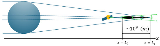
Figure 1.
Search geometry of an axion-like particle (ALP) lensing object using the stimulated backward reflection (SBR) method from a space probe (yellow). The blue circle denotes Earth, while the blue lines indicate the trajectories of individual ALPs incident from the left. The black triangular structure with trailing tails illustrates the concentrated distribution of dark matter at the focal region. The localized ALP flux is probed by a spherical wave of a coherent electromagnetic field to induce decay of the ALPs. denotes the emission point of the inducing field, and represents the effective terminal point beyond which the field strength becomes negligible. The total probing distance, , extends to approximately m.
Since the focal region lies beyond Earth’s atmosphere, it is natural to position the emission point of the inducing field in space in order to suppress background reflections arising from Rayleigh scattering. To maximize overlap with the densest portion of the ALP flux, it is preferable to locate the light source in proximity to the focal region, thereby directing the most intense part of the inducing field into the most concentrated region of the flux. Accordingly, deploying a space probe equipped with a coherent light source to the focal region and emitting the inducing field directly from the probe constitutes an effective strategy [14]. However, to thoroughly probe the concentrated ALP flux and to configure the inducing field as a near-ideal spherical wave, it is essential to determine an optimal observational position for the space probe based on the detailed structure of the gravitational lensing object. Moreover, in the previous work [14], the individual ALP velocity vectors around the focal region were not calculated at all despite its importance for evaluating the signal collection efficiency—a crucial factor in accurately estimating the sensitivity to ALP–photon coupling. Therefore, this paper addresses these essential issues through detailed numerical calculations.
In this paper, we discuss a conservative evaluation of the effective incident ALP density near Earth by assuming the S1 stream from the Cygnus constellation [15] in Section 2. We then provide the numerical method employed for this purpose in Section 3. In Section 4 we show the simulated result and discuss the resulting spatial structure of the focused ALP flux. In Section 5 we evaluate the acceptance factor of reflected signal photons based on the velocity distributions of the simulated ALP flux in individual segments over the propagation region of the inducing field. In Section 6 we provide a more accurate sensitivity projection based on the numerically calculated focused flux and the acceptance factor of reflected signal photons by taking the non-relativistic motion of the ALP flux due to the lensing effect into account. Section 7 concludes with a summary of the proposed Earth-lens telescope for distant ALP sources, while Section 8 presents future prospects along with supporting discussions.
2. A Model for Incident ALP Density Evaluation from Distant ALP-Emitting Objects
Reference [10] presents analytical expressions for both the focal length and the magnification of the axion-like particle (ALP) density along the incident axis, derived from geodesic trajectories under the Schwarzschild metric, in the case where a unidirectional ALP stream traverses Earth as illustrated in Figure 2. According to these formulations, for particles skimming Earth—i.e., those with trajectories outside its surface—the magnification is directly proportional to the impact parameter b, implying the potential for larger magnification relative to trajectories that penetrate Earth’s interior. However, the corresponding focal length increases as , thereby reducing the ALP density in the focal region with increasing b, which in turn diminishes the overall effectiveness of gravitational focusing. Conversely, for particles that pass through Earth’s interior, this focusing effect remains significant, as the focal length does not exhibit the same quadratic growth. In this study, we numerically evaluate the ALP density in the gravitational focal region, adopting the S1 stream originating from the Cygnus constellation [15] as a concrete astrophysical candidate for a unidirectional ALP flux traversing Earth’s interior. The rationale for selecting the S1 stream over the Galactic ALP halo lies in the intrinsic anisotropy of the former. While ALP halos may appear stationary in the Galactic rest frame, they are generally considered to be virialized, having attained a quasi-equilibrium state through gravitational interactions within the Galactic disk. As a result, their constituent particles exhibit thermal velocities on the order of the Galactic rotation speed. Thus, despite the Solar System’s motion at approximately 220 km/s relative to the Galactic center, the associated thermal dispersion of the ALPs prevents the assumption of a well-collimated, unidirectional flux incident on Earth. By contrast, dark matter associated with the observed S1 stream—an astrophysical structure presumed to be the remnant of a disrupted dwarf galaxy—passes through the Solar System with a bulk velocity of approximately 520 km/s [15]. Owing to the considerable distance to the progenitor system, which exceeds 8 kpc, the ALP flux originating from the S1 stream impinges upon Earth as a plane-parallel beam, exhibiting minimal angular divergence on the order of radians [14]. This exceptional collimation renders the flux highly susceptible to gravitational lensing effects, thereby enabling substantial concentration in the focal region.
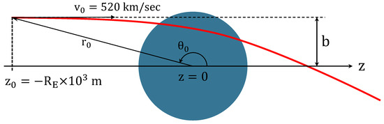
Figure 2.
Geometry of a particle trajectory, the initial position, the initial velocity, and the impact parameter. The ALP trajectory is shown with the red curve. The initial position is located at a distance of from Earth’s center along the incident axis z, and the vertical is offset by the impact parameter b. The initial velocity is km/s, directed parallel to the incident axis.
One of the authors of the present study previously calculated the effective average density of axion-like particle (ALP) incident on Earth’s gravitational lens, under the assumption that an ALP flux is streaming along the observed S1 stream in the earlier study [14]. This density estimate was then used to evaluate the sensitivity to ALP–photon coupling. However, the S1 stream serves merely as a representative example; the same framework is applicable to unknown, distant ALP sources as well.
As the simplest and most conservative estimate of the incoming ALP flux, we assume that the source emits ALPs isotropically, in analogy with distant stars emitting light. In this case, the farther the ALP source is from the Solar System—where the space probe is located—the smaller the solid angle subtended by the detector onboard the probe, leading to a reduced observed flux. Nevertheless, this narrowing of the solid angle also enables the identification of the source direction, effectively transforming the system comprising the planetary lens and the probe into a new type of telescope. Moreover, the planetary lens effect causes a convergence of the ALP flux along the line of sight to the source, introducing spatial anisotropy in the flux that can be exploited for directional ALP astronomy. In what follows, we formalize the effective average density of the ALP flux incident on Earth’s gravitational lens, assuming such a distant ALP-emitting object exists.
We thus introduce a conservative model on the ALP density at the incident plane in front of the Earth lens for a given incident stream velocity v. Suppose an ALP-emitting object such as a dwarf galaxy with the total energy which isotropically emits an ALP flux as a function of time t in the process of infall with corresponding to the total mass of the object. For a short time period compared to the infall time scale of the object, the emission rate can be approximated with the differential equation as a result of the emission of the ALP above the escape velocity . We assume because the age of the universe may be similar to the infall time scale. In this case the emission rate observed at the incident plane of the Earth lens with distance D to the source is approximated as
where the radius of the Earth , , and yr were used for the case of the S1-stream [14]. Given the incident rate, the local energy density flowing into a cylindrical volume with the base area corresponding to Earth’s cross-section in a short time duration is expressed as
We then assume that the velocity distribution of the ALP follows a Gaussian distribution, and the probe receives an ALP flux within the narrow solid angle. In this case the ALP energy density at the incident region around Earth is expressed with an effectively one-dimensional velocity dispersion as follows
where is integrated with the Gaussian weight in the case of a previous study [14], assuming that the escape velocity is km/s and the standard deviation is km/s as discussed in [15], resulting in
from Equation (3), which is conservative compared to with GeV/cm3 in [15]. We note that we can, in principle, distinguish the concentrated ALP flux from distant ALP-emitting objects based on the Doppler shift of the back reflected signal photons, as indicated in the first line of Equation (10), from those caused by the local dark matter halo following the standard halo model with km/s.
3. Method of the Numerical Calculation for the Gravitational Lensing Effect
In our calculation, the equations of motion for a Newtonian gravitational field generated by a uniformly dense Earth are reformulated into a finite-difference form using the Euler method and solved numerically. To exploit the spherical symmetry of the problem, we adopt spherical coordinates for the computation. Assuming a constant density profile for Earth’s interior, the gravitational potential forms inside and outside Earth with mass are given as follows:
where is the mass of an ALP, G is the gravitational constant, and is Earth’s radius. Based on Equation (5), the motion of the ALP follows the differential equations given below for the external and internal regions, respectively,
Here, j denotes the angular momentum per ALP mass. As evident from the second lines of Equations (6) and (7), angular momentum is conserved in the azimuthal () direction. The ALP trajectory thus can be limited to the two-dimensional plane , i.e., . While Equation (6) admits an analytical solution, Equation (7) does not. Therefore, to suppress computational errors on the surface of Earth, we perform numerical integration for both regions. The Euler form of the equations of motion is given as follows:
These difference equations enable the numerical integration of ALP trajectories across the interior and exterior of Earth under Newtonian gravity.
Next, we describe the initial conditions used in the following numerical calculation. As shown in Figure 2, the impact parameter b is varied from 0 to in 1000 equal steps. This gives us 1000 trajectories. From the geometry in Figure 2, the initial coordinate and velocity for a particle with a given b are given by
Here, and km/s, and these geometric relations are shown in Figure 2.
Figure 3 shows the particle trajectories obtained from the numerical calculation, visualizing how the paths bend and intersect in the x-z plane in Cartesian coordinates. Earth is positioned at the origin, centered at . It shows that the trajectories bend sharply near , while they remain nearly linear elsewhere. This indicates that the lensing effect is significant only in the vicinity of Earth. Furthermore, particles with larger impact parameters b exhibit longer focal lengths, while those with smaller b have shorter focal lengths.
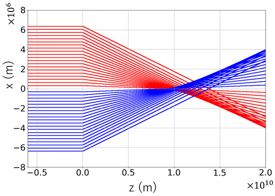
Figure 3.
Deflection of particle trajectories. Red curves correspond to trajectories with , while blue curves represent those with . The focal points are distributed in the range for the incident velocity of km/s.
4. Density Structure of an ALP Flux Focused by Gravitational Lensing of Earth
Performing the calculations described in the previous section, we generated 1000 particle trajectories for impact parameters in the range , with equal steps. To visualize the local ALP density at each spatial point, we discretized the region containing the gravitational lensing effect into discritized spatial elements. In this analysis, we adopt a cylindrical coordinate system with and , which naturally aligns with the rotational symmetry about the z-axis depicted in Figure 2. This coordinate choice is most suitable for capturing the cross-sectional density distribution of the lensing object. In the figure, strictly speaking, the x-axis corresponds to the cases of and . Nevertheless, since the azimuthal origin can be chosen arbitrarily, the -axis should be interpreted as representing an arbitrary cross-sectional plane around the z-axis. In all subsequent figures showing x–z cross-sections, this convention will be implicitly assumed. Due to rotational symmetry, trajectories with can be inferred by mirroring those with about the z-axis. Thus, one set of calculations yields double the statistical weight, enabling us to effectively obtain 2000 trajectories over the range .
Figure 4 shows the normalized density profile on the x-z plane of the lensing object when a unidirectional dark matter flux is incident along the z-axis with the velocity of 520 km/s. The element size is along the z-axis () and along the x-axis (). The number of trajectories in each segment is counted, and the density is obtained by dividing it by the segment volume. The density profiles in the color contour are displayed after normalizing individual densities to those of the maximum density segment. As shown in Figure 4, the spatial distribution of the normalized ALP density reveals a petal-like structure. In the surrounding regions, the density is also relatively high in the “petal” structures. This can be understood by analogy with an optical lens: light passing through a lens converges at the focal point and then diverges beyond it, forming high and low density regions. However, a major difference is that gravitational lensing in this context exhibits a large aberration relative to the focal length. Aberration refers to the spreading of rays due to imperfect focusing. As shown in Figure A3 in the Appendix A, the focal distance increases monotonically with the impact parameter b, introducing a significant variation. This dependence of aberration and focal length on b explains the emergence of the petal-shaped density structure beyond the focal region.
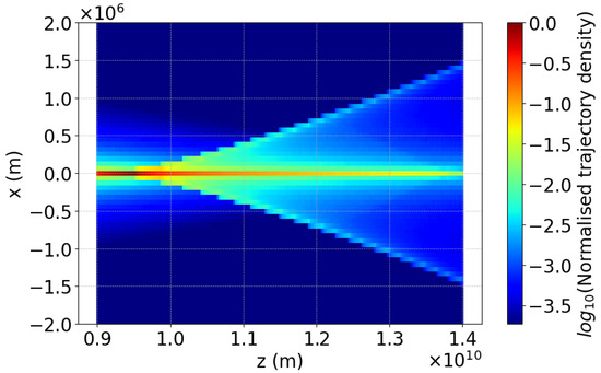
Figure 4.
Normalized density profile on the x-z plane of the lensing object when a unidirectional dark matter flux is incident along the z-axis with the velocity of 520 km/s.
5. Acceptance of Reflected Signal Photons on the Detector Plane
In the previous work [14] the acceptance factor —defined as the fraction of signal photons collected within the finite area of the detector plane—was roughly estimated by assuming ALPs moving at perpendicularly to the line of sight from the detector point, as a conservative approximation. In this paper, we refine the signal acceptance factor by considering ALPs traveling along curved trajectories. We thus derive the expression for based on Figure 5. We first summarize the kinematical relations of the induced decay. Let be the transverse distance from the optical axis at which a signal photon arrives on the detector plane. The interaction point between the inducing field and the ALP is denoted by . Accordingly, the angle between the local wavevector of the inducing field and the optical axis is . The angle definitions of the ALP velocity direction (black arrow) and the signal emission direction (blue arrow) at the induced decay point with respect to the local wavevector of the inducing field (red arrow) are illustrated in Figure 5, where the prime symbol indicates that the local reference coordinates are based on the direction of inducing field propagation with respect to the laboratory frame without the primed symbol.
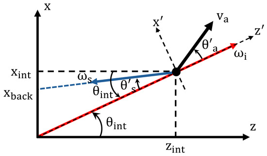
Figure 5.
Geometry of the inducing field emission point, the interaction point, and the signal photon trajectory. The red arrow indicates the wavevector of the inducing field. The blue arrow and dashed line represent the emission direction of the signal photon and the path to the detector plane, respectively. The black dot and the arrow denote the ALP and its velocity direction, respectively. Subscripts: “a” for the ALP, “i” for the inducing field, and “s” for the signal photon. The angles and represent the relative angles with respect to the wavevector of the inducing field.
In order to calculate , we first compute the emission angle of the signal photon at the decay point. Let be its relativistic velocity (c is the velocity of light), resulting in the Lorentz factor , and let be the energy of a single inducing photon. Energy–momentum conservation in the local reference frame requires the following relations:
From these, we can derive
It is allowed to put without the loss of generality with a constant fraction k if k satisfies the following relation:
as the result of energy–momentum conservation in Equation (10). This results in the mass independence of the decay angles because the mass in and are all canceled out in Equation (11). Therefore, counter-intuitively, the acceptance factor eventually becomes common for any ALP mass that we target. As shown in Figure 5, the coordinate value of the reflected signal photon on the detector plane is expressed as
In the following calculation to obtain the signal acceptance factor, a divergence angle of the inducing field, , propagating as the spherical wave was set to , and the searching distance is set to . Under these conditions, the distribution of the height from the center of the detector plane was obtained based on the numerically determined positions and velocities of individual simulated trajectories of ALPs over the searching distance.
Figure 6 shows the acceptance factor, , defined as the fraction of signal photons that are observed within a detector area of radius . The value of defines the integral range such that for counting the number of decayed photons observed within the detector area. The quantity is calculated using with in Equation (12). This acceptance factor is evaluated under the condition that the detector plane is placed at a distance of from Earth’s center and illuminated by a spherical inducing wave with a beam divergence angle of , over a search range of . The detector position corresponds to the location of the nearest focal point from Earth, calculated using the analytical expression for the focal length in Equation (A2) in the Appendix A, assuming an initial velocity of . The maximum value of among all the simulated trajectories with induced decays is approximately . Since the signal’s acceptance is calculated from discrete spatial points along the entire set of simulated ALP trajectories, the resulting values are also discrete. From Figure 6, it is found that approximately of the photons can be accepted using a detector of radius . This surprisingly high acceptance factor over the propagation distance of is attributed to the tight collimation of the ALP flux around the focal axis and the spherical mirroring effect of Earth on the wavefront of the inducing field.
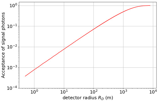
Figure 6.
Acceptance factor of collectible signal photons within detector radius as a function of . defines the integral range such that for counting the number of stimulated decay photons observed within the detector area. is calculated using with in Equation (12).
6. Sensitivity Projection on ALP–Photon Coupling
Given the focused ALP trajectories in the numerical calculation and the signal acceptance factor in the previous sections, we can move on to the calculation to evaluate the signal yield from SBR. For this calculation we move to spherical coordinates because the inducing field propagates as a spherical wave in space, which is expressed as the following equation [14]:
where specifies the volume scanned by the inducing field while it propagates over the searching region from radial position to along polar angle , assuming that the location of the space probe is at from the center of the Earth with the solid angle defined by the divergence angle determined by the specification of a coherent light source. The number density of the inducing field is parametrized as as a function of r reflecting the situation that the pulse center position moves along the r-axis with the surface area of at r.
In order to evaluate from the numerically generated trajectories, we divide the region of the focused ALP flux into segments in spherical coordinates instead of x-z coordinates as indicated in Figure 7. Accordingly the normalized density profile on the x-z plane is recalculated in spherical coordinates.
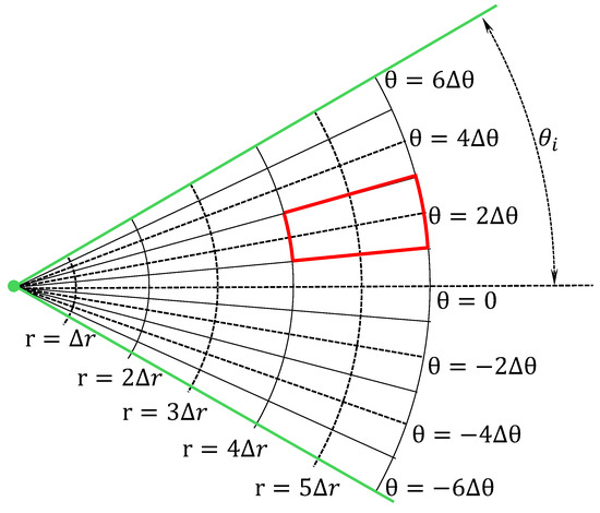
Figure 7.
Concept of segments in the propagation volume of an inducing field. The propagation region of the inducing field, as shown inside two green lines, is finely divided into segments with intervals and . This shows a configuration when the divergence angle of the inducing beam is divided into 12 equal angle ranges . The center of each segment takes values at . As an example, the segment outlined in red has its center at , and its boundaries are defined by the ranges and .
We introduce the initial ALP number density sourced by the S1 stream with Equation (4) as follows
We then introduce ALP densities in individual segment centers at as
where is the maximum density enhancement factor, in other words, the maximum magnification factor along the incident axis of the ALP flux, and is the number density of trajectories in the segment of the maximum magnification. The definition of magnification is provided in the Appendix A which summarizes the content of Ref. [10]. Given the volume of a segment for the inducing field as resulting from the rotation of the differential solid angle about the axis with in spherical coordinates, which is defined as
the number density of trajectories is expressed as
where is the number of trajectories in the inducing volume element , corresponding to with the number of trajectories counted in the plane in Figure 7.
The differential decay rate for the ALP decaying into two photons is given as follows [14]:
where is the ALP mass, is the ALP–photon coupling constant, is the energy of the inducing photon, and is a relative angle between the direction of the electric field component of the linear polarization of a decayed photon with respect to that of the magnetic field component of the linearly polarized inducing photons. We neglected the effect of the Lorentz boost of moving ALP due to the non-relativistic nature. Assuming with signal polarization selection in the detector part [14], the integral form in Equation (14) can thus be rewritten as an equivalent discrete summation as follows:
where the summation term enables the incorporation of the local overlap between the inducing field and the ALP density with
where is the energy of a single laser pulse, is the solid angel, and is the divergence angle of the inducing field.
In single-photon counting, we assume a photomultiplier tube (PMT) for the laser frequency. Although thermal noise in the PMT may remain as a residual background, the primary source of the background around the detector part in space is charged cosmic rays. At distances of approximately from the Earth, the dominant components are galactic cosmic rays. Among these, particles with energies above 1 GeV can enter the PMT photocathode at a flux of approximately . Assuming the photocathode area is on the order of , the expected rate of background photoelectron events due to cosmic rays is . In this work, we therefore estimate the background rate as .
Based on Equation (20), the observed number of signal photons via stimulated backward reflection (SBR) is expected to be
with T as the measurement time, f as the repetition rate of the inducing laser pulse, as photon detection efficiency, and as the acceptance factor. By equating the level of background fluctuations to the above observed signal yield, the upper limit of the coupling under the assumption of a null result is expressed as
with [14].
The parameters used for the sensitivity estimation are summarized in Table 1. Under these conditions, the projected sensitivity using the SBR method is shown in Figure 8. To contextualize the refined theoretical predictions presented in this work, we compare them with a representative set of experimental constraints widely referenced in the literature. The solid brown curve and the surrounding yellow band illustrate the expected parameter space from the benchmark QCD axion model, specifically the KSVZ model [16] with and . The dashed brown curve denotes the prediction from the DFSZ model [17,18] with . Cyan curves correspond to the ALP miracle model relevant to inflation [8], which was plotted for values of , 0.1, and 0.01. Shaded regions in the plot indicate existing exclusion limits from various experimental searches: vacuum magnetic birefringence (PVLAS [19], gray); light-shining-through-a-wall experiments (ALPS [20] and OSQAR [21], purple); penetrating scalar particle searches at the eV scale using the SPS neutrino beam (NOMAD [22], light cyan); the optical MUSE-faint survey [23] (blue); the solar helioscope experiment CAST [12] (green); two-beam stimulated resonant photon collider (SRPC) experiments—SAPPHIRES02 [24]—in quasi-parallel collision geometry (hatched red); and three-beam SRPC experiments, tSRPC00 [25], with the fixed incident angle setup (solid red).

Table 1.
Parameters used for the estimation of the sensitivity curve in Figure 8 assuming the laser-driven frequency range, that is, around the eV range which can cover the ALP mass range via for the inducing field.
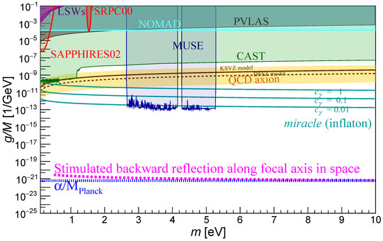
Figure 8.
Sensitivity projection with the stimulated backward reflection (SBR) method applied to the focused ALP flux by the Earth-lens effect, assuming the S1 stream as a distant ALP source. The megenta curve shows the expected upper limit based on this Earth-lens telescope concept with parameters summarized in Table 1. The other details are explained in the main text.
7. Conclusions
We envisioned a space observatory optimized for detecting distant ALP sources, considering the S1 stream as a concrete example of a remote source. The proposed telescope consists of Earth’s gravitational lens and a collector that captures stimulated backward reflections (SBRs) from remote ALP decay points illuminated by a spherically propagating laser field. First, we revealed the density structure of the focused ALP flux based on numerically simulated trajectories. Then, we established a computational scheme to evaluate the collection of reflected signal photons using the SBR method. Based on this telescope concept, we refined the sensitivity estimation in the eV mass range. This more accurate evaluation, which accounts for ALPs moving along curved trajectories, shows that the sensitivity can reach consistent with previously published results [14] based on rough approximations with similar parameters. Since the sensitivity to generic couplings is expected to reach values as small as this proposal demonstrates the feasibility of a novel space observatory capable of probing more distant ALP sources well beyond assuming, as one illustrative case, the DFSZ axion–photon coupling upper limit of in the eV mass range.
8. Future Prospects and Discussions
The existence of gravitationally bound axion or ALP configurations at distances of 10–100 from the Solar System is not only theoretically natural but under active observational investigation. The key points are summarized as follows:
- Axion miniclusters and axion stars are expected to be distributed throughout the Milky Way halo, including the 10–100 shell, especially in post-inflationary scenarios. Numerical studies show that a significant fraction of miniclusters survive stellar tidal disruption even at [26].
- These miniclusters can undergo Bose condensation in their cores to form axion stars, which may collapse and emit relativistic axions through processes such as bosenovae or gradual evaporation via self-interactions [27,28].
- Known magnetars in the Large Magellanic Cloud (LMC), such as SGR 0526-66 and J0456-69, located at ∼50 , serve as realistic candidates for ALP sources through photon–ALP conversion in strong magnetic fields [29].
- The historical core-collapse supernova SN 1987A in the LMC has already been used to constrain ALP emissions via neutrino duration and energy considerations [30].
From a detection perspective, ALPs emitted from the abovementioned sources may reach the Earth with a flux detectable by the proposed Earth-lens telescope. The proposed detection principle is applicable to inducing fields of any frequency. Currently available coherent electromagnetic sources on the ground can cover the range of to 10 eV, considering the physical dimensions of the sources. For instance, in the eV mass range, klystrons are commercially available. However, the available bandwidth, physical weight, and power consumption would pose realistic challenges for installing such sources on a space probe.
In our calculation, we have assumed a constant density for Earth and have neglected the effect of its slow rotation. Regarding the former simplification, although we plan to eventually incorporate Earth’s internal inhomogeneity with future upgrades in computational resources, reference [10] has already evaluated the effect and found that its impact on the focal length and magnification is not significant. On the other hand, the latter simplification can be justified by the following discussion. Based on the weak–field analysis of a rigidly rotating homogeneous sphere by Sereno (2003, Equations (21) and (22)) [31], the two transverse components of the deflection vector for a test particle that crosses the equatorial plane on a straight line ( at closest approach) are defined as the first order in spin J. The (scalar) spin parameter is the magnitude of the angular–momentum vector
which for a rigidly rotating body reduces to with representing the moment of inertia and representing the uniform angular velocity. For a homogeneous sphere , hence . Sereno works in geometrized units ; We restore explicitly in Equations (25) and (26). is a dimensionless spin parameter. We display only the terms that survive for : the frame-dragging contribution is then purely tangential.
where r and t denote, respectively, the radial (lens–centred) and tangential directions in the lens plane, and the upper (lower) sign corresponds to prograde (retrograde) motion. Introducing the physical velocity and restoring , the total deflection angle becomes
For the numerical estimate of Earth with , , , , Equations (24)–(26) give
so that Even for the slow ALP velocity , the Lense–Thirring shear is therefore nine orders of magnitude below static Schwarzschild bending, which can be safely ignored in the proposed setup. Since Earth’s spin effect is negligibly small, the incident angle dependence of the focal position is also negligibly small given the angle coverage of the inducing laser, rad.
The effect of Earth’s magnetic field via direct coupling to ALPs is expected to be negligibly small due to the low conversion probability for a coupling strength GeV−1, with T and . Unless the conversion probability approaches unity, the loss of the ALP flux cannot become a practical problem. On the other hand, the effect of charged particles near the detection region in the Van Allen belts may constitute a background source for the photon counter if the space probe is located within the belts. However, since the optimum detection position, m, from Earth’s center is much further than the maximum extent of the belts, m, this effect is also expected to be strongly suppressed.
Author Contributions
Conceptualization, K.H.; methodology, T.N.; software, T.N.; validation, K.H.; formal analysis, T.N.; data curation, T.N.; writing—original draft preparation, T.N. and K.H.; writing—review and editing, K.H.; visualization, T.N. and K.H.; supervision, K.H.; project administration, K.H.; funding acquisition, K.H. All authors have read and agreed to the published version of the manuscript.
Funding
This research was funded by the Collaborative Research Program of the Institute for Chemical Research at Kyoto University (Grant Nos. 2024-95 and 2025-100), the JSPS Core-to-Core Program (grant number: JPJSCCA20230003), and Grants-in-Aid for Scientific Research (Nos. and 24KK0068 and 25H00645) from the Ministry of Education, Culture, Sports, Science and Technology (MEXT) of Japan.
Data Availability Statement
Data are contained within the article.
Acknowledgments
T. Nakamura thanks Haruhiko Nishizaki for useful discussions on the efficiency and generality of the source code used for numerical computations and analysis, as well as on general relativity. K. Homma acknowledges the support of the Collaborative Research Program of the Institute for Chemical Research at Kyoto University (Grant Nos. 2024-95 and 2025-100), the JSPS Core-to-Core Program (grant number: JPJSCCA20230003), and Grants-in-Aid for Scientific Research (Nos. and 24KK0068 and 25H00645) from the Ministry of Education, Culture, Sports, Science and Technology (MEXT) of Japan.
Conflicts of Interest
The authors declare no conflict of interest.
Appendix A
Appendix A.1. Derivation of Magnification
The expression for , which is used to compute in Equation (16), and its derivation are given below. The geodesic calculation of massive particles passing through the Earth on the Schwarzschild metric is described as [10]
where denotes the mass enclosed within radius inside the Earth. The azimuthal angle near the gravitational lens is expressed as [10]
with the velocity of light c and , where are defined as follows:
where is the Schwarzschild radius of the Earth, b is the ALP’s impact parameter relative to the Earth, and v is the incident velocity. The deflection angle of the lens is then given by
From the geometry involving Earth’s center, the focal point of the lens, and the point of ALP incidence (as shown in Figure A1), the focal distance for an ALP incident with impact parameter b is given by

Figure A1.
Geometric relation between the focal distance and the impact parameter. The flux passing through the Earth is deflected by an angle , reaching a focal distance .
Figure A1.
Geometric relation between the focal distance and the impact parameter. The flux passing through the Earth is deflected by an angle , reaching a focal distance .

When a detector with radius is placed at a distance along the incident axis (the z-axis), the range of impact parameters for the flux passing through the detector is defined as . The magnification is expressed as the ratio between the area of the annular section of Earth’s cross-section corresponding to and the area of the detector. Specifically, it is given by [10]
The geometric relation for this configuration is illustrated in Figure A2.

Figure A2.
Conceptual diagram to define magnification . Shown are the detector placed along the incident axis (orange disk), the range of impact parameters for the flux passing through the disk (yellow annulus), and the trajectories corresponding to and (solid navy lines).
Figure A2.
Conceptual diagram to define magnification . Shown are the detector placed along the incident axis (orange disk), the range of impact parameters for the flux passing through the disk (yellow annulus), and the trajectories corresponding to and (solid navy lines).

Appendix A.2. Comparison of Numerical Calculation with the Analytical Prediction
Based on the analytical expression presented in the previous section, we calculate the focal length. The analytical formula used to compute the focal distance is given in Equation (A5). Using this expression, we perform the calculation for an incident velocity of and compare the results with those obtained from numerical integration. The comparison is shown in Figure A3, demonstrating that the numerical results reproduce the analytical solution with high accuracy.

Figure A3.
Dependence of the focal length F on the impact parameter b. The red dots in the upper plot show the focal length obtained from the numerical calculation, while the blue line shows the analytical computation given by Equation (A5). The black dots in the lower plot show the relative difference between numerical and analytical results, where , with .

References
- Peccei, R.D.; Quinn, H.R. CP Conservation in the Presence of Pseudoparticles. Phys. Rev. Lett. 1977, 38, 1440–1443. [Google Scholar] [CrossRef]
- Peccei, R.D.; Quinn, H.R. Constraints imposed by CP conservation in the presence of pseudoparticles. Phys. Rev. D 1977, 16, 1791–1797. [Google Scholar] [CrossRef]
- Wilczek, F. Problem of Strong P and T Invariance in the Presence of Instantons. Phys. Rev. Lett. 1978, 40, 279–282. [Google Scholar] [CrossRef]
- Weinberg, S. A New Light Boson? Phys. Rev. Lett. 1978, 40, 223–226. [Google Scholar] [CrossRef]
- Di Luzio, L.; Mescia, F.; Nardi, E.; Panci, P.; Ziegler, R. Astrophobic Axions. Phys. Rev. Lett. 2018, 120, 261803. [Google Scholar] [CrossRef] [PubMed]
- Badziak, M.; Harigaya, K. Naturally astrophobic QCD axion. J. High Energy Phys. 2023, 2023, 14. [Google Scholar] [CrossRef]
- Giannotti, M.; Irastorza, I.G.; Redondo, J.; Ringwald, A.; Saikawa, K. Stellar recipes for axion hunters. J. Cosmol. Astropart. Phys. 2017, 2017, 010. [Google Scholar] [CrossRef]
- Daido, R.; Takahashi, F.; Yin, W. The ALP miracle revisited. J. High Energy Phys. 2018, 2018, 104. [Google Scholar] [CrossRef]
- Yin, W.; Bessho, T.; Ikeda, Y.; Kobayashi, H.; Taniguchi, D.; Sameshima, H.; Matsunaga, N.; Otsubo, S.; Sarugaku, Y.; Tomomi, T.; et al. First Result for Dark Matter Search by WINERED. Phys. Rev. Lett. 2025, 134, 051004. [Google Scholar] [CrossRef]
- Prézeau, G. Dense Dark Matter Hairs Spreading out from Earth, Jupiter, and Other Compact Bodies. Astrophys. J. 2015, 814, 122. [Google Scholar] [CrossRef]
- Sikivie, P. Experimental Tests of the Invisible Axion. Phys. Rev. Lett. 1983, 51, 1415–1417, Erratum in Phys. Rev. Lett. 1984, 52, 695. [Google Scholar] [CrossRef]
- Anastassopoulos, V.; Aune, S.; Barth, K.; Belov, A.; Cantatore, G.; Carmona, J.M.; Castel, J.F.; Cetin, S.A.; Christensen, F.; Collar, J.I.; et al. New CAST Limit on the Axion-Photon Interaction. Nat. Phys. 2017, 13, 584–590. [Google Scholar] [CrossRef]
- Goodman, C.; Guzzetti, M.; Hanretty, C.; Rosenberg, L.J.; Rybka, G.; Sinnis, J.; Zhang, D.; Clarke, J.; Siddiqi, I.; Chou, A.S.; et al. ADMX Axion Dark Matter Bounds around 3.3 μeV with Dine-Fischler-Srednicki-Zhitnitsky Discovery Ability. Phys. Rev. Lett. 2025, 134, 111002. [Google Scholar] [CrossRef]
- Homma, K. Remote sensing of backward reflection from stimulated axion decay. J. High Energy Phys. 2024, 2024, 34. [Google Scholar] [CrossRef]
- O’Hare, C.A.J.; McCabe, C.; Evans, N.W.; Myeong, G.; Belokurov, V. Dark matter hurricane: Measuring the S1 stream with dark matter detectors. Phys. Rev. D 2018, 98, 103006. [Google Scholar] [CrossRef]
- Kim, J.E. Weak-Interaction Singlet and Strong CP Invariance. Phys. Rev. Lett. 1979, 43, 103–107. [Google Scholar] [CrossRef]
- Dine, M.; Fischler, W.; Srednicki, M. A simple solution to the strong CP problem with a harmless axion. Phys. Lett. B 1981, 104, 199–202. [Google Scholar] [CrossRef]
- Zhitnitsky, A.R. On Possible Suppression of the Axion Hadron Interactions. Sov. J. Nucl. Phys. 1980, 31, 260. (In Russian) [Google Scholar]
- Ejlli, A.; Della Valle, F.; Gastaldi, U.; Messineo, G.; Pengo, R.; Ruoso, G.; Zavattini, G. The PVLAS experiment: A 25 year effort to measure vacuum magnetic birefringence. Phys. Rep. 2020, 871, 1–74. [Google Scholar] [CrossRef]
- ALPS Collaboration; Ehret, K.; Frede, M.; Ghazaryan, S.; Hildebrandt, M.; Knabbe, E.A.; Kracht, D.; Lindner, A.; List, J.; Meier, T.; et al. New ALPS results on hidden-sector lightweights. Phys. Lett. B 2010, 689, 149–155. [Google Scholar] [CrossRef]
- OSQAR Collaboration; Ballou, R.; Deferne, G.; Finger, M., Jr.; Finger, M.; Flekova, L.; Hosek, J.; Kunc, S.; Macuchova, K.; Meissner, K.A.; et al. New exclusion limits on scalar and pseudoscalar axionlike particles from light shining through a wall. Phys. Rev. D 2015, 92, 092002. [Google Scholar] [CrossRef]
- NOMAD Collaboration; Astier, P.; Autiero, D.; Baldisseri, A.; Baldo-Ceolin, M.; Ballocchi, G.; Banner, M.; Bassompierre, G.; Benslama, K.; Besson, N.; et al. Search for eV (pseudo)scalar penetrating particles in the SPS neutrino beam. Phys. Lett. B 2000, 479, 371–380. [Google Scholar] [CrossRef]
- Regis, M.; Taoso, M.; Vaz, D.; Brinchmann, J.; Zoutendijk, S.L.; Bouché, N.F.; Steinmetz, M. Searching for light in the darkness: Bounds on ALP dark matter with the optical MUSE-faint survey. Phys. Lett. B 2021, 814, 136075. [Google Scholar] [CrossRef]
- SAPPHIRES Collaboration; Kirita, Y.; Airi, K.; Kensuke, H. Search for sub-eV axion-like particles in a quasi-parallel stimulated resonant photon-photon collider with “coronagraphy”. J. High Energy Phys. 2025, 06, 138. [Google Scholar] [CrossRef]
- Ishibashi, F.; Hasada, T.; Homma, K.; Kirita, Y.; Kanai, T.; Masuno, S.; Tokita, S.; Hashida, M. Pilot Search for Axion-Like Particles by a Three-Beam Stimulated Resonant Photon Collider with Short Pulse Lasers. Universe 2023, 9, 123. [Google Scholar] [CrossRef]
- Kavanagh, B.J.; Edwards, T.D.P.; Visinelli, L.; Weniger, C. Stellar Disruption of Axion Miniclusters in the Milky Way. Phys. Rev. D 2021, 104, 063038. [Google Scholar] [CrossRef]
- Levkov, D.G.; Panin, A.G.; Tkachev, I.I. Relativistic Axions from Collapsing Bose Stars. Phys. Rev. Lett. 2017, 118, 011301. [Google Scholar] [CrossRef]
- Fox, P.J.; Weiner, N.; Xiao, H. Recurrent Axion Stars Collapse with Dark Radiation Emission and Their Cosmological Constraints. Phys. Rev. D 2023, 108, 095043. [Google Scholar] [CrossRef]
- Fortin, J.F.; Gratton, M. Magnetar Hard X-Ray Emission from Axion-like Particle Conversion. J. Cosmol. Astropart. Phys. 2022, 2022, 009. [Google Scholar] [CrossRef]
- Raffelt, G.G.; Seckel, D. Bounds on Exotic Particle Interactions from SN 1987A. Phys. Rev. Lett. 1988, 60, 1793. [Google Scholar] [CrossRef]
- Sereno, M. Gravitational lensing by stars with angular momentum. Mon. Not. R. Astron. Soc. 2003, 344, 942–950. [Google Scholar] [CrossRef]


Disclaimer/Publisher’s Note: The statements, opinions and data contained in all publications are solely those of the individual author(s) and contributor(s) and not of MDPI and/or the editor(s). MDPI and/or the editor(s) disclaim responsibility for any injury to people or property resulting from any ideas, methods, instructions or products referred to in the content. |
© 2025 by the authors. Licensee MDPI, Basel, Switzerland. This article is an open access article distributed under the terms and conditions of the Creative Commons Attribution (CC BY) license (https://creativecommons.org/licenses/by/4.0/).