Abstract
We continue the analysis of the gauge-invariant decomposition of amplitudes in spontaneously broken massive gauge theories by performing the characterization of separately gauge-invariant subsectors for amplitudes involving trilinear interaction vertices for an Abelian theory with chiral fermions. We show that the use of Frohlich–Morchio–Strocchi gauge-invariant dynamical (i.e., propagating inside loops) fields yields a very powerful handle on the cancellations among unphysical degrees of freedom (the longitudinal mode of the massive gauge field, the Goldstone scalar and the ghosts). The resulting cancellations are encoded into separate Slavnov–Taylor invariant sectors for 1-PI amplitudes. The construction works to all orders in perturbation theory. This decomposition suggests a novel strategy for the determination of finite counter-terms required to restore the Slavnov–Taylor identities in chiral theories in the absence of an invariant regularization scheme.
1. Introduction
Gauge-invariant fields of the Frohlich–Morchio–Strocchi (FMS) type [1,2] provide a consistent and gauge-invariant description of spontaneously broken gauge theories [3]. They are related to the original fields via an invertible field redefinition [4]. This ensures physical equivalence with the standard formulation in terms of elementary non-gauge-invariant fields, since the physical observables, including the S-matrix elements, do not depend on the specific field parameterization chosen, provided that the asymptotic states are left unaffected. This is a general result of Quantum Field Theory known as the Equivalence Theorem [5,6,7,8,9]. Physical equivalence can also be proven directly by cohomological arguments [10].
Gauge-invariant fields exhibit several desirable properties. They are associated with positive spectral density [11,12], as should be expected for a physical description of these excitations. This is in contrast with the ordinary scalar field used to describe the Higgs mode, whose Källén–Lehmann representation is not gauge-invariant and exhibits a non-positive spectral density.
Unfortunately, power-counting renormalizability is, in general, not manifest when using gauge-invariant fields [4], due to their composite nature. However, it turns out that power-counting renormalizability can be retained provided one uses appropriate Lagrange multipliers embedded into the so-called BRST doublets [13,14] in order to enforce a field change in the variables, as discussed in [10,15,16].
Moreover, gauge-invariant fields allow for the effective control of the physical content of the Slavnov–Taylor (ST) [17,18,19] identities, a crucial set of functional relations for the vertex functional that generate the one-particle irreducible (1-PI) amplitudes of the model, which ensures the cancellation of unphysical intermediate states associated with the quartet mechanism [20,21,22].
In fact, each 1-PI amplitude can be expanded according to the number of internal Higgs fields and the number of vector meson gauge-invariant fields. It turns out that separate ST identities hold for the different sectors , i.e., physical unitarity cancellations occur independently in each sector.
This natural yet technically non-trivial property has been proven in ref. [15] with the Algebraic Renormalization approach [23,24]. Explicit examples were presented for ST identities involving two-point 1-PI amplitudes in the Abelian Higgs–Kibble model with chiral fermions.
In the present paper we take one step further and extend the diagrammatic analysis of the FMS gauge-invariant formalism to ST identities involving three-point 1-PI amplitudes.
In particular we check the fulfillment of the sector-by-sector ST identities for the UV-divergent parts of the fermionic amplitudes in an Abelian chiral model.
The main motivation for this is that for chiral theories, no symmetric regularization scheme is known to preserve the ST identities at the regularized level, due to the presence of the matrix, and so one has to work out finite symmetry-restoring counter-terms order by order in the loop expansion [25].
One may hope that the FMS gauge-invariant formalism can provide some guidance to identify a general strategy in order to obtain these finite counter-terms.
As a preliminary step toward this goal, we check, in the present paper, the fulfillment of the ST identities for the UV-divergent parts of the 1-PI amplitudes and describe in detail the underlying cancellation mechanism.
As is well-known, at one loop order, UV divergences have to fulfill the ST identities, with the ambiguities in the regularization procedure only affecting finite one-loop counter-terms. Thus, the UV-divergent parts of the amplitudes provide a very clean basis to understand the sector decomposition holding true in the FMS formalism.
First of all let us consider amplitudes without external fermion legs. For these amplitudes it is clear that fermion loops always contribute to the -sectors, while -sectors, where either or is greater than zero, are unaffected by fermionic contributions. So for those sectors, one can safely use naive Dimensional Regularization with an anticommuting matrix in order to ensure the fulfillment of the ST identities already at the regularized level.
On the other hand, one-loop amplitudes involving external fermion legs contain one fermionic chain. Therefore, one in general obtains contributions from those chains to all -sectors due to insertions on the chain of scalar, ghost and gauge propagators.
In this case several new aspects arise. Cancellations among unphysical states in these latter sectors can be analytically traced and display an interesting structure, as will be explicitly shown.
Moreover, the relevant set of one-loop ST identities involves both three-point and two-point 1-PI functions. However, their projection on the sectors yields a set of algebraic relations where the two-point functions only appear in sectors with . This is because at one loop, there are obviously at most two internal lines in a two-point 1-PI amplitude, so these amplitudes cannot simply contribute to sectors with (at one loop order, three point functions have at most three internal lines).
This seemingly obvious fact has deep implications in the problem of the restoration of the ST identities broken by intermediate regularization and is tied to the locality properties of the theory.
In fact, finite counter-terms, required to restore the ST identities, can also be decomposed according to the -grading. Therefore, finite counter-terms, modifying the two-point 1-PI amplitudes, will only affect the relevant ST identities’ projections to which two-point amplitudes actually contribute. In the sector , one has to work out finite counter-terms affecting the three point functions directly.
We will present explicit results for the full set of finite symmetry-restoring counter-terms, derived by exploiting such a decomposition, in a separate publication. The present paper is devoted to describing the sector decomposition structure of UV divergences.
The paper is organized as follows. In Section 2 we review the FMS gauge-invariant formalism in its BRST version and describe the ST identity decomposition on separately invariant sectors. In Section 3 we make a connection with the standard formalism and establish a dictionary between the FMS and the conventional amplitudes. In Section 4 we consider two-point ST identities. Section 5 contains a detailed analysis of selected fermionic three-point ST identities and their substructure, while Section 6 presents an analysis of ST identities involving three-point bosonic amplitudes. Finally, our conclusions are presented in Section 7. The appendices contain the tree-level vertex functional and the propagators (Appendix A), the functional identities of the theory (Appendix B) and the explicit results for the UV-divergent part of the relevant amplitudes involved (Appendix C).
2. The Model
We consider an Abelian Higgs–Kibble model with chiral fermions in the gauge-invariant formalism of [15].
The Frohlich–Morchio–Strocchi (FMS) gauge-invariant fields are denoted by h and :
where ∼ denotes on-shell equivalence when the equations of motions for the Lagrange multipliers X and ,
enforcing the relevant constraints on the fields , are imposed [15]. The operator is defined in Equation (A2).
In the above equations is the Higgs complex field, represents the physical scalar mode and represents the Goldstone field. v is the vacuum expectation value (v.e.v.). Moreover,
is the covariant derivative, with e being the coupling constant and the Abelian gauge field. The fields are on-shell equivalents to the FMS gauge-invariant fields originally proposed in [1,2].
A comment is in order here. The most general solution to Equation (2) is
where are free fields satisfying the equations
Perturbatively, one can safely choose the solution . This can be easily seen by integrating out the auxiliary fields and noticing that the determinant of the differential operators drops out upon integration over the antighost and ghost fields:
i.e., the determinants arising from the -function are exactly compensated (modulo inessential multiplicative factors) by the integration over the Grassmann variables and . A formal proof of these results has been given in [16].
At variance with the approach discussed in [4], power-counting renormalizability remains manifest. The technical reason can be ascribed to the presence of suitable derivative operators multiplying the Lagrange multipliers once the latter are embedded into BRST doublets [13,14]. In perturbation theory they do not affect the equivalence to the original theory, as can be seen both formally in the path-integral formalism by integrating out the Lagrange multipliers and in a mathematically rigorous approach using BRST techniques [15,16,23].
In cohomological language, this is to say that the Lagrange multipliers only enter via a BRST-exact term [14].
It turns out that the only dim.5 and dim.6 interaction terms in the classical vertex functional in Equation (A1) are those proportional to the Lagrange multipliers X and . The propagators and are, however, vanishing, so power-counting violating interaction vertices involving are harmless. Moreover, the potentially dangerous interaction term still does not violate power-counting renormalizabilty, due to the fact that the propagators and fall off as , as one can see from Equation (A7).
Thus, the model offers a power-counting renormalizable version of the FMS construction.
The 1-PI vertex functional obeys the following Slavnov–Taylor (ST) identity:
This functional identity holds as a consequence of the classicalBRST symmetry of the gauge-fixed classical action
where is the ghost field, and the antighost. b is the Nakanishi–Lautrup field, while are chiral fermions.
The BRST transformations of , being non-linear in the quantized fields, have to be defined by coupling them in the tree-level vertex functional to the antifields [19,26]. The complete classical vertex functional , including the antifield-dependent terms and external sources required to define the functional equations of motion for the Lagrange multipliers, is given in Equation (A1).
is the generating functional of the 1-PI amplitudes of the theory, namely
where represents a field or an external source, the sum is over the loop index n and all r-tuples of length , and is a combinatorial factor (for instance, in the case of three fields of the same type, ). is the 1-PI generating functional of 1-PI amplitudes at order n in the loop expansion.
One can further expand the 1-PI Green’s functions according to the number of gauge-invariant fields h and the combination given by Equation (A12), i.e.,
In the above equation we have denoted the functional derivative as
and have suppressed, for notation simplicity, the space–time dependence of the fields and external sources .
is the sum of n-loop diagrams contributing to the 1-PI amplitude with external legs and containing internal h-propagators and internal -propagators. is the sum of n-loop diagrams contributing to the 1-PI amplitude without internal h- and -propagators.
One could in fact also choose not to use the combination in Equation (A12), but instead use in Equation (A8) and again achieve the decomposition of amplitudes according to . We choose , since Feynman rules on the diagonal basis are simplified with this choice.
The crucial result of [15] is that the ST identities in Equation (6) do not actually hold only for the full 1-PI amplitudes , but also hold separately for each -sector, namely
In the present paper we will specialize to the one-loop order so that there are no contributions from the bilinear terms in the last two lines of Equation (11).
Moreover, we will consider the Landau gauge and set the additional mass parameter m in Equation (A1) to zero. There is no loss in generality in making such a choice. m is an additional parameter allowed by the symmetries of the theory and the power-counting, yet it is unphysical and will disappear once one recovers the amplitudes in the standard formalism, as has been extensively checked in [27].
Thus, one can conveniently set for the purpose of studying the sector-by-sector ST identity fulfillment in the simplest-possible setting.
In the Landau gauge, ghosts are free, so there are no one-loop corrections to the BRST transformations of the fields of the theory, i.e.,
where the dots stand for any number of internal fields and external sources of the model.
Thus, the tower of -ST identities simplifies to
3. Recovering the Amplitudes in the Conventional Formalism
In order to recover the one-loop 1-PI amplitudes in the conventional formalism, we need to eliminate the auxiliary fields and . The procedure works as follows. Using Equations (A16) and (A17), we see that for the n-loop vertex functional , only depends on the combinations
On the other hand, by going on-shell with at the tree-level, according to Equations (A15) and (A19), we get, respectively,
where in the first equation, we use the tree-level on-shell condition
The latter equation has the solution
which is used in the first part of Equation (16). The most general solution to Equation (17) is given by
with being a Klein–Gordon massive field. However, at the perturbative level, one cansafely neglect the field , as has been discussed at length in [16].
We conclude that for the one-loop order, going on-shell with the extended pairs of fields and in order to make contact with amplitudes in the standard formalism requires (i) disregarding all one-loop amplitudes involving , as a consequence of the condition in the second part of Equation (16), and (ii) replacing the source with the combination
4. ST Identities for Two-Point Amplitudes
We review here the analysis of the ST identities for two-point amplitudes. Unlike in the computations presented in [15], where use is made of internal off-diagonal propagators on a symmetric basis, we recover here the same results by using the mass eigenstate propagators.
The reason is that mass eigenstate propagators are more suited to the automation of one- and higher-loop computations via tools like FeynArts/FormCalc [28,29]. Of course both bases are equivalent. In order to switch from the mass eigenstate basis to the symmetric one, Equations (A6) and (A12) are used. One sees from these equations that the symmetric Green functions involving only , and coincide with those with external legs , and .
In the present paper we will explicitly check the fulfillment of the ST identities sector-by-sector for the UV-divergent part of the relevant 1-PI amplitudes. We will work in Dimensional Regularization with anticommuting . While this regularization scheme is known to be inconsistent (for a recent review see [25]), it gives the correct results for UV divergences in the one-loop order. In a separate publication we will discuss the renormalization of the model in the Breitenlohner–Maison–’t Hooft’–Veltman (BMHV) scheme and the construction of sector-by-sector finite counter-terms for restoring the ST identities broken by the intermediate regularization.
The ST identities to be considered for two-point 1-PI functions are obtained by taking one derivative with respect to the ghost and then with respect to and , respectively, and then setting all fields and external sources to zero. We obtain the two identities
to be verified in each -sector. Since they involve two-point amplitudes, .
As a preliminary remark, we notice that in order to study the contributions from diagrams involving and , it is useful to move to the variables
From Equation (A5) one sees that the diagonal propagators and are vanishing, while the off-diagonal propagator reads
Therefore non-vanishing contributions from diagrams involving can only arise through interaction vertices involving both and . Now the field obviously depends only on and h. Through direct inspection, one therefore sees that in the tree-level vertex functional Equation (A1), all interaction vertices only depend on (and thus on ), with the exception of the vertex (we specialize here to the case of interest ).
Therefore, all diagrams involving and cancel each other out with the exception of those involving the vertex in Equation (24).
We now discuss each identity in turn, labeled according to the fields over which functional differentiation is taken.
4.1. -STI
There are four sectors to be considered, namely , , and .
Sector
The -sector is spanned by diagrams with no internal h and -lines.
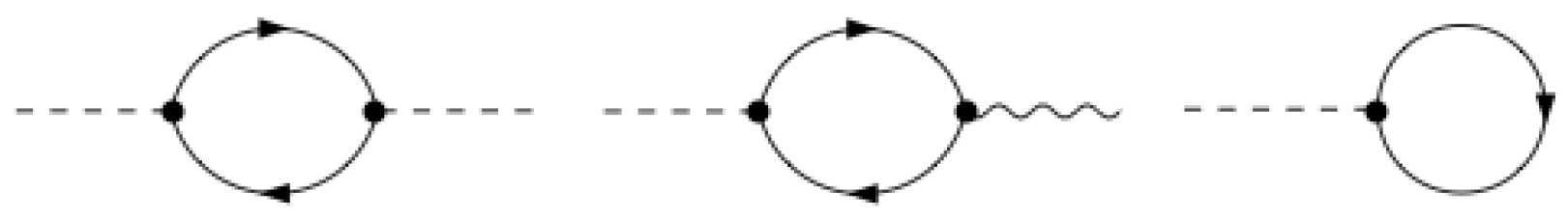
Diagrams involving internal and -lines and no vertices of the type used in Equation (24) cancel each other out, and thus, they can be safely dropped in the subsequent analysis. For instance, the diagrams in Figure 1 cancel out since the interaction vertices are the same, while the propagators of (dashed red line) and (dashed blue line) have opposite signs.
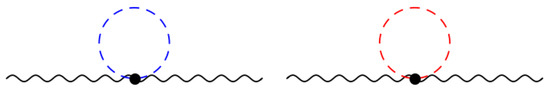
Figure 1.
Diagrams contributing to mutually compensating. The dashed red line represents the -propagator, and the dashed blue line the -propagator.
Moreover, since we are in Landau gauge and the Goldstone fields are massless, in Dimensional Regularization there are no contributions from Goldstone tadpoles.
In Dimensional Regularization the only non-vanishing diagrams in and are the fermionic bubbles depicted in Figure 2.
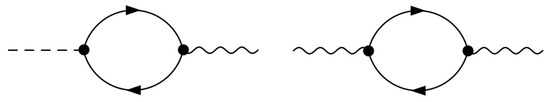
Figure 2.
Non-vanishing amplitudes in and .
4.2. Sectors , and
4.3. -STI
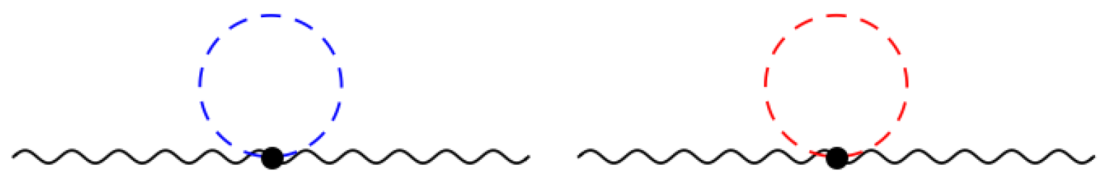
As in the case of -STI, there are four sectors to be considered, namely , , and . Fermion contributions appear only in the sector via the diagrams depicted in Figure 3.

Figure 3.
Fermion bubbles contributing to the sector of the -ST identity.
Again, cancellations between diagrams involving , and no vertices in Equation (24) are at work.
By repeating the analysis and through the direct inspection of Equations (A23), (A24) and (A26), one can check that the ST identities
are verified for each relevant -sector.
We notice that, being a tadpole with just one internal line, does not contribute to the sector . This means that in this sector, the ST identity reduces to
i.e., the highest-order sector only involves amplitudes with the same greatest number of external legs.
A comment is in order here. The components and of and , respectively, contain dimension 3 terms and dimension 4 terms that violate power-counting renormalizability.
However, in the sums and , they cancel each other out. This is a consequence of the fact that power-counting renormalizability is violated in each sector, yet the sum of all sectors must obey bounds imposed by power-counting renormalizability, since the full theory is power-counting renormalizable.
5. Slavnov–Taylor Identities for Fermionic Amplitudes
By taking a functional derivative of Equation (13) with respect to , and and then setting all fields and external sources to zero, one obtains the set of identities in momentum space:
At one loop order the relevant sectors to be considered are , , and . Let us consider each of them in detail.
5.1. Sector
This sector is spanned by all diagrams involving one internal -propagator and one internal h-propagator. There are no such diagrams contributing to the two-point function , so the ST identity reduces to
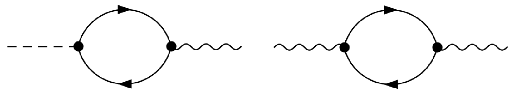
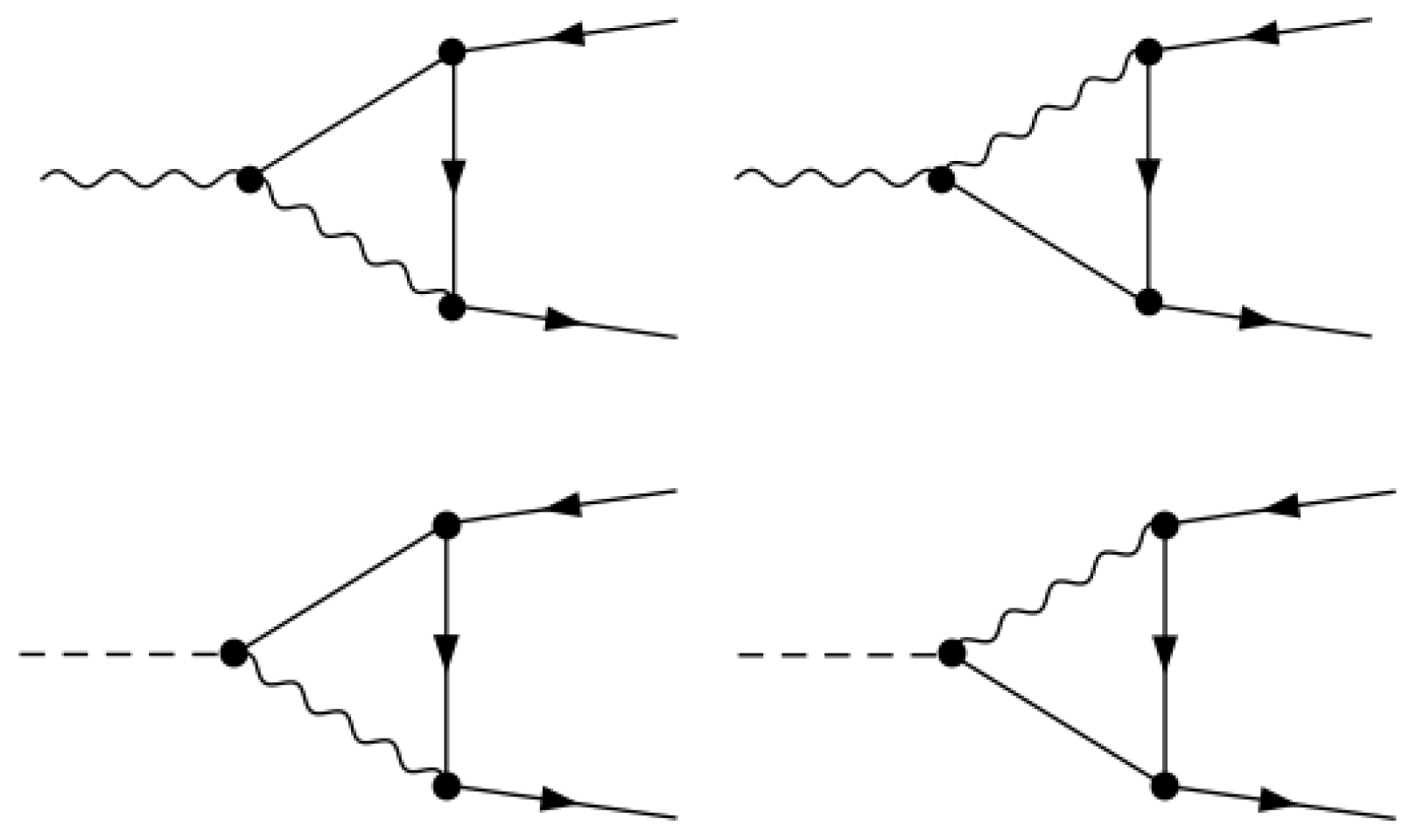
The diagrams to be considered are depicted in Figure 4. We observe, first of all, that according to Equation (A8), the symmetric function is equal to the amplitude in the mass eigenstate basis .

Figure 4.
Diagrams contributing to the -sector at amplitudes (first line) and (second line). The internal wavy lines are -propagators, and the solid lines h-propagators.
In order to see how the cancellations embodied in Equation (29) work diagrammatically, we notice that the fermion chain is the same in both diagrams in each column in Figure 4.
Thus, we can focus on the product of the trilinear vertices with the -propagator. One finds from Equation (A1), after going to the mass eigenstate basis, that
and
In addition, one has to take into account the prefactor in the second term of the Slavnov–Taylor identity Equation (29). So one finds the following (p is the momentum of the h-propagator coming into the vertex):
where in the second line we use the fact that .
Similarly, one finds, for the diagrams with an external gauge line contracted with the incoming momentum k, that
By summing Equations (32) and (33), one gets
since
This shows that the ST identity Equation (29) is indeed satisfied.
Explicit values of the UV-divergent parts of the relevant amplitudes are reported in Appendix C. It is interesting to see that these diagrams are also indeed UV-divergent, as a consequence of the derivative interactions in the classical action Equation (A1). For instance, the form factor UV coefficients reported in Equation (A32) individually exhibit a more severe degree of divergence than expected in power-counting renormalizable theory (according to which should have a UV degree of at most 1, in fact zero according to Lorentz-covariance). , and contains terms of order , and and terms of order .
Nevertheless the sum of all contributions must obey the power-counting renormalizable bound and thus must have a UV dimension of zero. One can check, through the direct inspection of Equation (A32), that this is indeed the case. This is a highly non-trivial check that must hold true as a consequence of the special manifest power-counting renormalizability of the present formalism.
5.2. Sectors and
In these sectors the two-point amplitude also contributes. The analysis can be carried out along the same lines for all sectors (, and ). Also here, for general arguments one can aptly resort to the symmetric basis, while automated explicit computations for each sector are carried out on a diagonal basis.
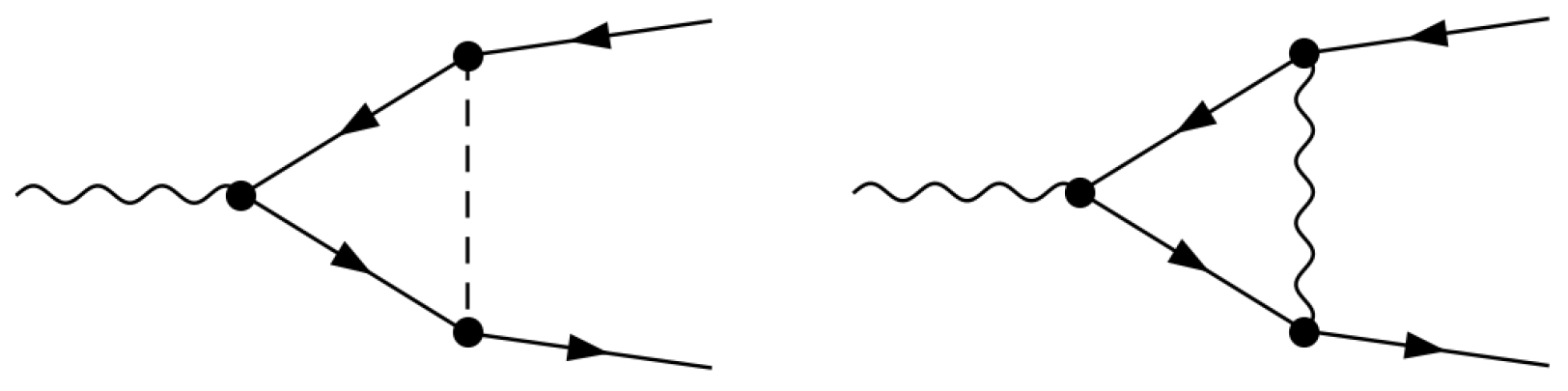
Let us start from diagrams with three fermion interaction vertices, as depicted in Figure 5.

Figure 5.
Diagrams with three fermion interaction vertices. The dashed line denotes -propagators, and the wavy line denotes the -propagator.
They can be written schematically as
where can be either h, , or . Notice that the fermions only interact with the scalar and not with X, so there are no diagrams involving .
The combination
can be simplified by using the tree-level ST identity
on the relevant tree-level 1-PI Green’s function in the first two amplitudes of Equation (36).
By taking into account that
and momentum conservation is , one ends up with the identity
where
i.e., the ST identity holds true for this particular subset of diagrams in the sector .
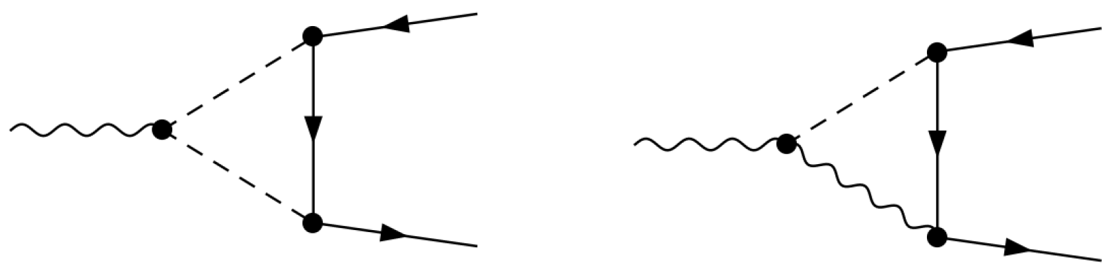
The analysis of diagrams with two fermion interaction vertices displayed in Figure 6 follows the same lines as described in the previous subsection.

Figure 6.
Diagrams with two fermion interaction vertices. In the left diagrams one line is always a Goldstone , while the second one can denote -propagators. The wavy line denotes the -propagator.
One can explicitly check the fulfillment of the ST identity for the UV-divergent parts of the relevant amplitudes, sector-by-sector, by using the results reported in Appendix C.
6. Slavnov–Taylor Identities for Bosonic Amplitudes
We list here the set of Slavnov–Taylor identities involving the trilinear interaction vertices obtained by taking one derivative with respect to , , and , , , respectively:
Each Slavnov–Taylor identity in Equation (42) can be further decomposedinto the sectors
The various contributions can be classified according to the value of the sum . Since the ST identities involve trilinear amplitudes, this sum can be at most 3. In this latter case the possible contributions are classified according to the sectors , , and .
One sees, according to the Feynman rules of the theory, that there are no contributions from the sectors and . Moreover, there are no contributions from the two-point amplitudes to the sectors where (because obviously the two-point amplitudes at one loop can have at most two internal lines).
When , the relevant sectors are , and . There are contributions to all of the amplitudes, as can be seen from the explicit computations of the UV-divergent part of these amplitudes reported in Appendix C.
When , the sectors to be considered are and . Finally there is the -sector, containing all amplitudes without any internal h and -lines, including the fermion bubbles.
In momentum space the first part of Equation (43) is given by
Equation (43) reads
Momentum conservation implies that (all momenta are consideredto be incoming) and that the support of the two-point functions is restricted to the hyperplane for the two-point amplitude and amplitude, and to the hyperplane for the two-point amplitude. We have explicitly verified all of the relevant ST identities in each sector through direct computations.
The results for the UV-divergent terms are reported in Equations (A24)–(A26), (A32), (A34) and (A35).
As far as finite symmetry-restoring counter-terms are concerned, the above remarks imply that if the highest value of the sum equals 3, only trilinear amplitudes must be corrected. This fact is not manifest in the full ST identity; see Equation (42).
Similarly, when it comes to sectors with , no tadpole contributions can enter.
By exploiting this fact one can arrange finite counter-terms in layers and have guidance in order to evaluate them sector-by-sector. Detailed results will be presented in a separate publication.
7. Conclusions
In this paper we have illustrated the fulfillment of ST identities sector-by-sector in gauge-invariant variables by focusing on the UV-divergent terms of the relevant amplitudes at one loop order. We have investigated the simplest non-trivial ST identities involving trilinear vertices both for bosonic and for fermionic amplitudes.
The explicit evaluation of the UV divergences of the theory shows that power-counting renormalizability is lost within each sector, due to the presence of higher-derivative interactions, yet the model remains power-counting renormalizable, so the sum of the different sector decompositions yields a manifestly power-counting renormalizable amplitude.
This is a very advantageous and peculiar property of the gauge-invariant formalism proposed in [15], which does not hold in general for models implementing gauge-invariant FMS fields [4].
Since the ST identities hold true sector-by-sector, one can renormalize each sector independently. In particular, sectors without fermions do not suffer from the absence of a consistent invariant regularization scheme in chiral theories. Notice that the notion of gauge-invariant sectors holds true to all orders in perturbation theory and provides the appropriate mathematical framework to discuss separately invariant subsets of diagrams.
We have also shown that for ST identities only involving external bosonic legs (and possibly ghosts, in gauges different from Landau), the fermionic contributions are restricted to the -sector. On the other hand, amplitudes with external fermion legs present contributions to all admissible sectors.
Therefore, a consistent regularization scheme, fulfilling the ST identities in chiral gauge theory, can be defined by using naive Dimensional Regularization in all sectors unaffected by the presence of fermions and by adopting, e.g., the BMHV scheme in the remaining sectors plus the corrections due to finite symmetry-restoring counter-terms.
The explicit evaluation of such counter-terms will be presented in a separate publication, as will the extension of the formalism to non-Abelian gauge theories.
Funding
This research was partially funded by INFN.
Data Availability Statement
The original contributions presented in this study are included in the article. Further inquiries can be directed to the corresponding author.
Acknowledgments
Useful discussions with Dominik Stockinger and Thomas Hahn are gratefully acknowledged.
Conflicts of Interest
The author declares no conflicts of interest.
Appendix A. Tree-Level Effective Action
The full tree-level effective action is
The operator in Equation (A1) is given by
for and by
for the case. In the present paper we will focus only on the Landau gauge .
Diagonalization of the quadratic part in the scalar sector is obtained by the following field redefinitions:
The propagators on a mass eigenstate basisare
One gets back the original symmetric basis via the fieldtransformations
The propagators on a symmetric basis are
In a similar fashion, diagonalization of the vector–scalar quadratic part is achieved by the following field redefinition [15]
The non-vanishing mass eigenstate propagators are given by
The transverse and longitudinal tensors are defined as
We notice that the dependence on of in Equation (A8) is via the combination , so one can avoid introducing interaction vertices depending on by using the field instead of . Still, the propagators are diagonal, and one has
i.e., a purely transverse propagator, as expected. The inverse field transformation is given by
We notice, according to the last part of Equation (A12), that is also gauge-invariant.
We adopt these mass eigenstate fields in the automation of the calculation of 1-PI amplitudes by using FeynArts/FormCalc [28,29].
Appendix B. Functional Identities
The vertex functional is the generating functional of the 1-PI amplitudes of the theory. It can be expanded according to the loop order n as
is the tree-level effective action (including the external sourcesfor composite operators) given in Equation (A1).
- The X- and h-equations of motionThe tree-level effective action obeys the following identities:Since the r.h.s of the above equations is linear in the quantized fields, both identities hold true at the quantum level, i.e.,The first equation implies that the whole dependence of thevertex functional on X happens via the combination , while the dependence on the field h is confined at the tree-level (on the symmetric basis we are using here).
- The - and -equations of motionalso obeys the following identities:Based on a similar argument, they translate at the quantum level toThe last equation implies that the dependence on the field is confined at the tree-level (on the symmetric basis we are using here), while the first onesuggests that the dependence on only happens via the combination , to all orders in the loop expansion.
Appendix C. Sector Decomposition of UV Divergences
We list here the sector decomposition of the UV-divergent parts for the relevant 1-PI amplitudes. UV-divergent parts are denoted by the same amplitude barred.
For fermionic amplitudes the chirality projectors are defined as
while . All Dirac matrices are understood in . The amplitudes are evaluated in Dimensional Regularization with .
Appendix C.1. The Tadpole
Appendix C.2. The Two-Point Goldstone Amplitude
Appendix C.3. The Two-Point Higgs Amplitude
Appendix C.4. The Two-Point Mixed Goldstone-Gauge Field Amplitude
Appendix C.5. The Two-Point Gauge Field Amplitude
Appendix C.6. The Two-Point Fermion Amplitude
We introduce the following form factors:
Then,
Appendix C.7. The Three-Point Gauge-Scalar Amplitude
The UV-divergent contribution is written in terms of the following form factors:
In the sector the only non-vanishing form factor is
Moreover,
The form factors in the sectors , , and vanish.
Appendix C.8. The Three-Point Gauge-Goldstone-Scalar Amplitude
The UV-divergent contribution is written in terms of the following form factors:
We have
The form factors in the sectors , , and vanish.
Appendix C.9. The Three-Point Scalar-Goldstone Amplitude
The sector decomposition is given by ()
Appendix C.10. The Three-Point Fermion-Goldstone Amplitude
We introduce the form factor decomposition
The form factors are
Appendix C.11. The Three-Point Fermion-Gauge Amplitude
In a similar way we define ()
The form factors are
References
- Frohlich, J.; Morchio, G.; Strocchi, F. Higgs phenomenon without a symmetry breaking order parameter. Phys. Lett. B 1980, 97, 249–252. [Google Scholar] [CrossRef]
- Frohlich, J.; Morchio, G.; Strocchi, F. Higgs phenomenon without symmetry breaking order parameter. Nucl. Phys. B 1981, 190, 553–582. [Google Scholar] [CrossRef]
- Maas, A. Brout-Englert-Higgs physics: From foundations to phenomenology. Prog. Part. Nucl. Phys. 2019, 106, 132–209. [Google Scholar] [CrossRef]
- Boeykens, B.; Dudal, D.; Oosthuyse, T. Equivalence theorem at work: Manifestly gauge-invariant Abelian Higgs model physics. Phys. Rev. D 2025, 111, 045007. [Google Scholar] [CrossRef]
- Kamefuchi, S.; O’Raifeartaigh, L.; Salam, A. Change of variables and equivalence theorems in quantum field theories. Nucl. Phys. 1961, 28, 529–549. [Google Scholar] [CrossRef]
- Bergere, M.C.; Lam, Y.M.P. Equivalence Theorem and Faddeev-Popov Ghosts. Phys. Rev. D 1976, 13, 3247–3255. [Google Scholar] [CrossRef]
- Blasi, A.; Maggiore, N.; Sorella, S.P.; Vilar, L.C.Q. Renormalizability of nonrenormalizable field theories. Phys. Rev. D 1999, 59, 121701. [Google Scholar] [CrossRef]
- Ferrari, R.; Picariello, M.; Quadri, A. An Approach to the equivalence theorem by the Slavnov-Taylor identities. J. High Energy Phys. 2002, 4, 033. [Google Scholar] [CrossRef]
- Cohen, T.; Forslund, M.; Helset, A. Field Redefinitions Can Be Nonlocal. arXiv 2024, arXiv:2412.12247. [Google Scholar] [CrossRef]
- Binosi, D.; Quadri, A. Renormalizable extension of the Abelian Higgs-Kibble model with a dimension-six operator. Phys. Rev. D 2022, 106, 065022. [Google Scholar] [CrossRef]
- Dudal, D.; van Egmond, D.M.; Guimaraes, M.S.; Holanda, O.; Palhares, L.F.; Peruzzo, G.; Sorella, S.P. Gauge-invariant spectral description of the U(1) Higgs model from local composite operators. J. High Energy Phys. 2020, 2, 188. [Google Scholar] [CrossRef]
- Dudal, D.; van Egmond, D.M.; Guimaraes, M.S.; Palhares, L.F.; Peruzzo, G.; Sorella, S.P. Spectral properties of local gauge invariant composite operators in the SU(2) Yang–Mills–Higgs model. Eur. Phys. J. C 2021, 81, 222. [Google Scholar] [CrossRef]
- Barnich, G.; Brandt, F.; Henneaux, M. Local BRST cohomology in gauge theories. Phys. Rept. 2000, 338, 439–569. [Google Scholar] [CrossRef]
- Quadri, A. Algebraic properties of BRST coupled doublets. J. High Energy Phys. 2002, 5, 051. [Google Scholar] [CrossRef]
- Quadri, A. Gauge-invariant quantum fields. Eur. Phys. J. C 2024, 84, 975, Erratum in Eur. Phys. J. C 2024, 84, 1073. [Google Scholar] [CrossRef]
- Binosi, D.; Quadri, A. Off-shell renormalization in the presence of dimension 6 derivative operators. Part I. General theory. J. High Energy Phys. 2019, 9, 032. [Google Scholar] [CrossRef]
- Slavnov, A.A. Ward Identities in Gauge Theories. Theor. Math. Phys. 1972, 10, 99–107, Erratum in Theor. Math. Phys. 1972, 10, 153. [Google Scholar] [CrossRef]
- Taylor, J.C. Ward Identities and Charge Renormalization of the Yang-Mills Field. Nucl. Phys. 1971, B33, 436–444. [Google Scholar] [CrossRef]
- Weinberg, S. The Quantum Theory of Fields. Vol. 2: Modern Applications; Cambridge University Press: Cambridge, UK, 2013. [Google Scholar] [CrossRef]
- Becchi, C.; Rouet, A.; Stora, R. The Abelian Higgs-Kibble Model. Unitarity of the S Operator. Phys. Lett. 1974, B52, 344–346. [Google Scholar] [CrossRef]
- Kugo, T.; Ojima, I. Manifestly Covariant Canonical Formulation of Yang-Mills Field Theories: Physical State Subsidiary Conditions and Physical S Matrix Unitarity. Phys. Lett. 1978, B73, 459–462. [Google Scholar] [CrossRef]
- Curci, G.; Ferrari, R. An Alternative Approach to the Proof of Unitarity for Gauge Theories. Nuovo Cim. 1976, A35, 273. [Google Scholar] [CrossRef]
- Piguet, O.; Sorella, S.P. Algebraic renormalization: Perturbative renormalization, symmetries and anomalies. Lect. Notes Phys. Monogr. 1995, 28, 1–134. [Google Scholar] [CrossRef]
- Grassi, P.A.; Hurth, T.; Steinhauser, M. Practical algebraic renormalization. Ann. Phys. 2001, 288, 197–248. [Google Scholar] [CrossRef]
- Bélusca-Maito, H.; Ilakovac, A.; Kuehler, P.; Mador-Bovzinovic, M.; Stoeckinger, D.; Weisswange, M. Introduction to Renormalization Theory and Chiral Gauge Theories in Dimensional Regularization with Non-Anticommuting γ5. Symmetry 2023, 15, 622. [Google Scholar] [CrossRef]
- Gomis, J.; Paris, J.; Samuel, S. Antibracket, antifields and gauge theory quantization. Phys. Rept. 1995, 259, 1–145. [Google Scholar] [CrossRef]
- Binosi, D.; Quadri, A. Off-shell renormalization in the presence of dimension 6 derivative operators. II. Ultraviolet coefficients. Eur. Phys. J. C 2020, 80, 807. [Google Scholar] [CrossRef]
- Hahn, T. Generating Feynman diagrams and amplitudes with FeynArts 3. Comput. Phys. Commun. 2001, 140, 418–431. [Google Scholar] [CrossRef]
- Hahn, T. Automatic loop calculations with FeynArts, FormCalc, and LoopTools. Nucl. Phys. Proc. Suppl. 2000, 89, 231–236. [Google Scholar] [CrossRef]
Disclaimer/Publisher’s Note: The statements, opinions and data contained in all publications are solely those of the individual author(s) and contributor(s) and not of MDPI and/or the editor(s). MDPI and/or the editor(s) disclaim responsibility for any injury to people or property resulting from any ideas, methods, instructions or products referred to in the content. |
© 2025 by the author. Licensee MDPI, Basel, Switzerland. This article is an open access article distributed under the terms and conditions of the Creative Commons Attribution (CC BY) license (https://creativecommons.org/licenses/by/4.0/).