Massive Graviton from Diffeomorphism Invariance

Abstract

In this work, we undertake a comprehensive study of the functional measure of gravitational path integrals within a general framework involving non-trivial configuration spaces. As in Riemannian geometry, the integration over non-trival configuration spaces requires a metric. We examine the interplay between the functional measure and the dynamics of spacetime for general configuration-space metrics. The functional measure gives an exact contribution to the effective action at the one-loop level. We discuss the implications and phenomenological consequences of this correction, shedding light on the role of the functional measure in quantum gravity theories. In particular, we describe a mechanism in which the graviton acquires a mass from the functional measure without violating the diffeomorphism symmetry nor including Stückelberg fields. Since gauge invariance is not violated, the number of degrees of freedom goes as in general relativity. For the same reason, Boulware–Deser ghosts and the vDVZ discontinuity do not show up. The graviton thus becomes massive at the quantum level while avoiding the usual issues of massive gravity.

1. Introduction

General relativity and the standard model have both been extremely successful in describing fundamental phenomena. Nonetheless, many problems in the interface of gravity and high-energy physics, such as the dark sector and singularities, cannot be explained by either of these theories. This has led to a plethora of attempts to modify these models.

One interesting modification of general relativity regards massive gravity. Attempts to give the graviton a mass date back to the 30s [1], but it was only recently that consistent theories of massive gravity have been found [2,3,4,5,6] (see also Ref. [7] for an in-depth review). A massive graviton indeed introduces many issues, such as the violation of diffeomorphism (gauge) invariance, the van Dam–Veltman–Zakharov (vDVZ) discontinuity, and the presence of Boulware–Deser ghosts [8]. Gauge invariance can be reinstated via Stückelberg fields, which is legitimate but does require new degrees of freedom. The vDVZ discontinuity [9,10], namely the disagreement with general relativity in the massless limit, is usually conjectured to be solved at the non-linear regime by the Vainshtein screening mechanism [11,12]. Only a few models have successfully implemented the Vainshtein mechanism [12,13,14,15,16], which can also bring along the possibility of superluminal velocities [3,15,17,18,19,20].

In this paper, we propose a novel procedure to give the graviton a mass without introducing any of the aforementioned issues and without modifying classical general relativity. Our finding is based on a non-trivial path-integral measure, which is required for obtaining gauge-invariant correlation functions. The functional measure introduces non-linear loop corrections, which act as a gravitational potential and result in a (quantum) mass for the graviton in the linear regime. The most important point is the preservation of the diffeomorphism invariance, which is responsible for keeping the theory free of ghosts and of the vDVZ discontinuity. The so obtained mass is, however, pure imaginary, thus precluding the existence of gravitons as asymptotic states.

This paper is organized as follows. In Section 2, we review some aspects of the functional measure in quantum field theory. The one-loop correction induced by the functional measure is then studied in Section 4, where the graviton mass is calculated. Comparison with experimental data yields stringent bounds on the model. In Section 5, we obtain Newton’s potential and discuss its consequences. Finally, we draw our conclusions in Section 6.

We shall here adopt DeWitt’s notation, commonly used in the functional approach of quantum field theory. In this notation, we use:

(i) 

capital Latin letters (e.g., $I,J,K,\dots$) to denote general discrete indices, including spacetime and/or internal indices. For example, a non-Abelian gauge vector would read $A_{\mu }^a=A^I$ for $I=\{a,\mu \}$;

(ii)

lowercase mid-alphabet Latin indices (such as $i,j,k,\dots$) for both discrete and continuum indices (spacetime points), e.g., $i=(I,x)$. For example, a non-Abelian gauge field would read $A_{\mu }^a=A^i$ for $i=\left(\right\{a,\mu \},x)$;

(iii)

repeated lowercase indices account for sums and integrations:

$$A^i{B}_i=\int {\mathrm{d}}^{4}x\sqrt{-g}\sum _I{A}^I\left(x\right)B_I\left(x\right),$$

(1)

for arbitrary tensor fields $A^i$ and $B^i$.

2. Functional Measure in Quantum Field Theory

Functional methods play a major role in quantum field theory. At the perturbative level, they are equivalent to canonical quantization, but otherwise they offer a breadth of techniques well suited for non-perturbative calculations in gauge theories and quantum gravity. Indeed, one could arguably define a quantum field theory by the path integral, from which everything else would follow.

However, functional integrals still suffer from formal constructions and manipulations. This is mainly due to the divergences that ought to be renormalized (which result in an additional prescription) and to the elusive functional integration measure. At the level of the rigour of physics, these are generally overlooked because regularization and renormalization are seen as an essential part of the understanding of the quantum realm. While, most of the time, this is a good practical way to make physical predictions, it may miss important physics, hinged on a proper definition of the path integral.

The issue of divergences can be partially sorted out by adopting Wilson’s effective field theory. In this case, the path integral is defined by a finite quantum theory with a physical cutoff $\mathsf{\Lambda }$ [21,22,23] (see also [24,25] for introductory reviews):

$$Z_{\mathsf{\Lambda }}\left[J\right]={\int }_{\mathsf{\Omega }\left(\mathsf{\Lambda }\right)}\mathrm{d}\mu \left[\phi \right]e^{i\left(S\left[{\phi }^i\right]+J_i{\phi }^i\right)}.$$

(2)

The action

$$S\left[{\phi }^i\right]=S_{\mathrm{classical}}+S_{\mathrm{GF}}+S_{\mathrm{ghost}}$$

(3)

includes the classical action $S_{\mathrm{classical}}$, gauge-fixing terms $S_{\mathrm{GF}}$ and the ghost action $S_{\mathrm{ghost}}$. We use the notation ${\phi }^i={\phi }^I\left(x\right)$ for arbitrary fields, namely

$${\phi }^i=(\varphi \left(x\right),A_{\mu }\left(x\right),g_{\mu \nu }\left(x\right),{\overline{c}}_{\mu }\left(x\right),c^{\mu }\left(x\right),\dots ),$$

(4)

which includes ghosts fields ${\overline{c}}_{\mu },c^{\mu }$. Integration over $g_{\mu \nu }$ is defined operationally via the background field method, where one writes $g_{\mu \nu }\to g_{\mu \nu }+h_{\mu \nu }$ in terms of a background $g_{\mu \nu }$ and the quantum field $h_{\mu \nu }$. As usual, $h_{\mu \nu }$ is a gauge field1, whose gauge transformation is ${\delta }_{\xi }{h}_{\mu \nu }={\nabla }_{(\mu }{\xi }_{\nu )}$, and its corresponding ghosts are assumed to be included in Equation (4). Mimicking the mathematical theory of integration on manifolds, one could regard the integration as taking place in some portion $\mathsf{\Omega }\left(\mathsf{\Lambda }\right)\subset \mathcal{M}$ of the infinite-dimensional manifold of fields, hereby denoted $\mathcal{M}$ and called configuration space. The subset $\mathsf{\Omega }\left(\mathsf{\Lambda }\right)$ corresponds to the integration domain of interest, only including field configurations with energies below $\mathsf{\Lambda }$ that satisfy some required boundary conditions and represent the elements of the equivalence class under gauge transformations. We stress that, in the Wilsonian effective field theory, the cutoff $\mathsf{\Lambda }$ corresponds to a physical scale (e.g., atomic spacing, string scale, etc.), which makes the theory manifestly finite. This precludes the need for the cancelation of divergences. Because $\mathsf{\Lambda }$ corresponds to some physical scale, it is not supposed to be sent to infinity. The continuum limit $\mathsf{\Lambda }\to \infty$ indeed only exists when the theory is renormalizable, for which there must be a fixed point of the renormalization group flow. Renormalization in the Wilsonian sense is just a statement about the separation of scales, for which physics at energies $E\ll \mathsf{\Lambda }$ does not depend on $\mathsf{\Lambda }$. Wilson’s renormalization group, namely

$$\mathsf{\Lambda }{\displaystyle \frac{d{Z}_{\mathsf{\Lambda }}\left[J\right]}{d\mathsf{\Lambda }}}=0,$$

(5)

then tells us how the theory gets modified as one changes the cutoff so that low-energy physical observables remain $\mathsf{\Lambda }$-independent.

In generalized field coordinates covering $\mathsf{\Omega }$, one should expect the measure to take the form [26,27,28,29]:

$$\mathrm{d}\mu \left[\phi \right]=\mathcal{D}{\phi }^i\sqrt{\mathrm{Det}{G}_{ij}},$$

(6)

where $\mathcal{D}{\phi }^i={\prod }_i\mathrm{d}{\phi }^i$ and $\mathrm{Det}{G}_{ij}$ denotes the functional determinant of some metric $G_{ij}$ of the configuration space2. The factor $\mathcal{D}{\phi }^i$ includes the measures of all fields, including Faddeev–Popov ghosts. In uncondensed notation:

$$\mathcal{D}{\phi }^i=\prod _x\prod _{\mu ,\rho <\sigma }\mathrm{d}\varphi \left(x\right)\mathrm{d}{A}_{\mu }\left(x\right)\mathrm{d}{g}_{\rho \sigma }\mathrm{d}{\overline{c}}_{\mu }\mathrm{d}{c}^{\mu }\dots .$$

(7)

Very much like in Riemannian geometry, the factor $\sqrt{\mathrm{Det}{G}_{ij}}$ is required to guarantee the invariance under change of coordinates in $\mathsf{\Omega }$. Note that, from this geometrical construction, such changes of coordinates are field redefinitions commonly used in quantum field theory. Since physics should not depend on the way we parameterize the fields, the measure (6) is required even for a flat configuration space. Furthermore, being that gauge transformations are a special kind of field redefinition, the presence of $\sqrt{\mathrm{Det}{G}_{ij}}$, along with a connection in configuration-space [30], is of utmost importance to make the quantum theory consistent. On the other hand, we stress that, because the configuration space is just an abstract space with no direct physical meaning, structures defined upon it, such as the configuration-space metric $G_{ij}$, bear no physical interpretation. However, such geometrical structures are required to make sense of the path integral, ultimately affecting physical observables.

The functional measure forces upon us the introduction of the metric $G_{ij}$. There is no general physical prescription for choosing such a metric, hence one must view $G_{ij}$ as part of the definition of the theory. The quantum theory is fully determined by the ordered pair $(\mathcal{L},G_{ij})$, formed by the classical Lagrangian and the configuration-space metric. We thus see that different choices of $G_{ij}$ for the same classical Lagrangian lead to different quantum theories. A typical widespread procedure is to identify $G_{ij}$ from the bilinear form appearing in the classical Lagrangian [30,31,32,33,34]. This choice singles out a unique quantum theory but, while legitimate, it lacks physical motivation.

One should not fear such indeterminacy of the configuration-space metric. The classical Lagrangian shares the same freedom. In general, only two guiding principles are used for determining $\mathcal{L}$: (i) locality and (ii) symmetry. In the Wilsonian spirit, these allow the Lagrangian to be written as an infinite expansion of operators invariant under the underlying symmetry. We shall adopt the very same principles for $G_{ij}$. Locality, or more precisely ultralocality, requires:

$$G_{ij}=G_{IJ}{\delta }^{\left(4\right)}(x,x^{\prime }),$$

(8)

where $G_{IJ}=G_{IJ}\left(\phi \right)$ is the metric on the subspace $\mathcal{N}\subset \mathcal{M}$ of homogeneous field configurations. Here the condensed indices are $i=(I,x)$, $j=(J,x^{\prime })$. The Dirac delta enforces the same metric $G_{IJ}$ across all spacetime points. Symmetry, on the other hand, is used to write $G_{IJ}$ as an expansion in inverse powers of cutoff $\mathsf{\Lambda }$ (see Appendix A). Note that, by construction, $G_{ij}$ depends only on physical fields and not on ghost fields.

The additional term from the functional measure in Equation (6) can be written as a correction to the classical action by using $log \mathrm{Det}=\mathrm{Tr} log$, thus:

$$\begin{array}{cc}\hfill \mathrm{Det}{G}_{ij}& =e^{\mathrm{Tr} log G_{ij}}\hfill \\ \hfill & =e^{\int {\mathrm{d}}^{4}x\sqrt{-g}\mathrm{tr} log G_{ij}{|}_{x=x^{\prime }}},\hfill \end{array}$$

(9)

where the functional trace is defined by:

$$\mathrm{Tr} A_{IJ}(x,x^{\prime })=\int {\mathrm{d}}^{4}x\sqrt{-g} \mathrm{tr} A_{IJ}(x,x)$$

(10)

and tr denotes the ordinary trace over the discrete indices $I,J$. Because discrete (e.g., $I,J$) and continuous (e.g., $x,x^{\prime }$) indices are independent, $G_{IJ}\left(\phi \right){\delta }^{\left(4\right)}(x,x^{\prime })$ is the component of a tensor product in configuration space. The Dirac delta is the coordinate representation of the identity $\mathbb{I}$ in the position basis. Therefore, the configuration-space metric can be written as $G\otimes \mathbb{I}$, where $G=G_{IJ}\mathrm{d}{\phi }^I\otimes \mathrm{d}{\phi }^J$. For arbitrary matrices A and B, the well-known identity

$$log(A\otimes B)=log\left(A\right)\otimes {\mathbb{I}}_B+{\mathbb{I}}_A\otimes log\left(B\right)$$

(11)

gives:

$$log(G\otimes \mathbb{I})=log\left(G\right)\otimes \mathbb{I}.$$

(12)

In coordinates, we thus obtain:

$$log\left[G_{IJ}{\delta }^{\left(4\right)}(x,x^{\prime })\right]=log\left(G_{IJ}\right){\delta }^{\left(4\right)}(x,x^{\prime }).$$

(13)

Using Equation (13) in Equation (9) leads to:

$$\mathrm{Det}{G}_{ij}=e^{{\delta }^{\left(4\right)}\left(0\right)\int {\mathrm{d}}^{4}x\sqrt{-g} \mathrm{tr} log{G}_{IJ}},$$

(14)

with the abbreviated notation ${\delta }^{\left(4\right)}\left(0\right)\equiv {\delta }^{\left(4\right)}(x,x)$.

One should note that Equation (14) is divergence-free due to the presence of the Wilsonian cutoff $\mathsf{\Lambda }$. However, it requires the use of some representation of the Dirac delta to make sense of ${\delta }^{\left(4\right)}\left(0\right)$. We shall adopt the Gaussian representation:

$${\delta }^{\left(4\right)}\left(x\right)={\displaystyle \frac{{\mathsf{\Lambda }}^4}{{\left(2\pi \right)}^2}}{e}^{{\displaystyle \frac{-x^2{\mathsf{\Lambda }}^2}{2}}},$$

(15)

for which ${\delta }^{\left(4\right)}\left(0\right)=\frac{{\mathsf{\Lambda }}^4}{{\left(2\pi \right)}^2}$. Using (14), (15), and the ordinary identity tr $log=logdet$ , we find [35]:

$$Z_{\mathsf{\Lambda }}\left[J\right]=\int \mathcal{D}{\phi }^i{e}^{i\left(S_{\mathrm{eff}}\left[{\phi }^i\right]+J_i{\phi }^i\right)},$$

(16)

with the Wilsonian effective action

$$S_{\mathrm{eff}}=\int {\mathrm{d}}^{4}x\sqrt{-g}\left(\mathcal{L}-i{\displaystyle \frac{{\mathsf{\Lambda }}^4}{2{\left(2\pi \right)}^2}}logdet{G}_{IJ}^{\mathsf{\Lambda }}\right),$$

(17)

for some bare Lagrangian $\mathcal{L}$ (which includes gauge-fixing and ghost terms). Equation (17) is the most general expression regardless of the fields present in the theory. As we shall see below, for most typical choices of $G_{IJ}^{\mathsf{\Lambda }}$ involving the spacetime metric $g_{\mu \nu }$, one is able to reproduce a mass-like term in the effective action.

Obtaining a more manageable action requires specifying the fields and symmetries present in the Lagrangian so that one can determine $det{G}_{IJ}^{\mathsf{\Lambda }}$. As a first approximation, we shall restrict ourselves to the lowest order in ${\mathsf{\Lambda }}^{-1}$, which for all kinds of fields in curved spacetime leads to (see Appendix A and Ref. [36]):

$$det{G}_{IJ}^{\mathsf{\Lambda }}=A{(-det{g}_{\mu \nu })}^B,$$

(18)

where $A,B$ are dimensionless constants that take different values for different fields present in the configuration-space metric $G_{IJ}^{\mathsf{\Lambda }}$. Hence, from Equation (18), the most general configuration-space metric for arbitrary fields yields [36,37,38]:

$$S_{\mathrm{eff}}=\int {\mathrm{d}}^{4}x\sqrt{-g}\left(\mathcal{L}-i{\displaystyle \frac{B{\mathsf{\Lambda }}^4}{2{\left(2\pi \right)}^2}}log(-det{g}_{\mu \nu })-i{\displaystyle \frac{{\mathsf{\Lambda }}^4}{2{\left(2\pi \right)}^2}}logA\right).$$

(19)

After variation, the second term in Equation (19) produces a cosmological-constant like term (see Equation (45) below), which can absorb the last term in (19) by a redefinition of B. Therefore, in the rest of the paper, we shall simply set $A=1$ without any loss of generality. We see that B plays the role of a coupling constant. As we shall see later, the renormalization group (5) will induce a $\mathsf{\Lambda }$-dependence $B=B\left(\mathsf{\Lambda }\right)$ so as to keep the graviton mass $\mathsf{\Lambda }$-independent. We also note that, unlike the continuum formalism ($\mathsf{\Lambda }\to \infty$), where power divergences are cancelled and only logarithmic ones correspond to physical effects, powers of $\mathsf{\Lambda }$ are not cancelled out in the Wilsonian renormalization group. Indeed, they play a crucial role in the correct understanding of the running of coupling constants with $\mathsf{\Lambda }$.

One can see that the corrections from the functional measure in Equation (19) are imaginary. We stress that this is not a problem. Indeed, imaginary terms in the effective action only signal vacuum instabilities. These instabilities can be understood via Schwinger’s pair production mechanism, in which the vacuum decays into a particle–antiparticle pair with probability [39,40,41,42,43]:

$$P=1-e^{-2\mathrm{Im}\left(S_{\mathrm{eff}}\left[g_{\mathrm{sol}}\right]\right)},$$

(20)

with $g_{\mathrm{sol}}$ some solution to the equations of motions. The details of the by-products of such decay depends on the fields present in the fundamental Lagrangian $\mathcal{L}$. For example, if there are no fields other than the metric, the vacuum decays into a couple of gravitons since the graviton is its own antiparticle.

In spite of the form of the correction, we stress that Equation (19) does not violate diffeomorphism invariance. The apparent violation results from the fact that $\sqrt{\mathrm{Det}{G}_{ij}}$ transforms as a (functional) scalar density, thus so does the last term in Equation (19). However, the $\mathcal{D}{\phi }^i$ also transforms as a scalar density in such a way that the full measure $\mathcal{D}{\phi }^i\sqrt{\mathrm{Det}{G}_{ij}}$ is invariant. Therefore, variations of the apparent symmetry-breaking term under spacetime diffeomorphisms are canceled by the functional Jacobian that shows up from $\mathcal{D}{\phi }^i$, keeping the quantum theory and all observables invariant3. Because the functional measure and the classical action are invariant under diffeomorphisms, the background-field effective action $\mathsf{\Gamma }\left[g\right]$ naturally reflects such symmetry. In fact, at the one-loop level it reads

$$\begin{array}{cc}\hfill \mathsf{\Gamma }\left[{\phi }^i\right]& =S\left[{\phi }^i\right]-{\displaystyle \frac{i}{2}}log\mathrm{Det}{G}_{ij}+{\displaystyle \frac{i}{2}}log\mathrm{Det}{\mathcal{H}}_{ij}\hfill \end{array}$$

(21)

$$\begin{array}{cc}\hfill & =S\left[{\phi }^i\right]+{\displaystyle \frac{i}{2}}log\mathrm{Det}{\mathcal{H}}_j^i,\hfill \end{array}$$

(22)

where the configuration-space metric $G_{ij}$ enters the usual correction $log\mathrm{Det}{\mathcal{H}}_{ij}$, transforming the bilinear map ${\mathcal{H}}_{ij}=S_{,ij}$, whose determinant is basis-dependent, into a linear operator ${\mathcal{H}}_j^i$, whose determinant is invariant [28,45]. Therefore, diffeomorphism invariance is respected, but not manifested in the action (19) before computing the path integral. It is only after the path integral is calculated and the standard one-loop correction $log\mathrm{Det}{\mathcal{H}}_{ij}$ included that the result becomes manifested invariantly. As we stressed before, this should not be surprising, since one must take the path integral Jacobian into account and not just transform the action (with the measure correction) alone. The Jacobian cancels out the apparent non-covariant term from the correction in (2.10), leaving the whole theory gauge invariant as it should. As shown in Equation (22), a manifested gauge invariance result is possible, but comes at the cost of specifying the classical Lagrangian ${\mathcal{L}}_{\mathrm{classical}}$ so that the path integral can be performed. We shall see an example of this in Section 3 (see Equation (31)). It is precisely this fact that allows for a mass for the graviton while respecting gauge invariance, be it manifested or not.

We should also comment about other existing approaches in the literature. In Refs. [46,47], the authors take the measure as fixed, not considering Jacobians in the path integral. They assess the diferences in diferent choices of field parameterizations, in which case would generally result in different quantum theories. We instead follow the more general approach by DeWitt [27] (see also [45,48]), where the measure is not kept fixed, instead it transforms as any integration measure would under a change of variables. Hence, in our case, the factor $\sqrt{\mathrm{Det}{G}_{ij}}$ is required to account for such changes as one normally encounters in the theory of integration on manifolds. The Jacobian from $\mathcal{D}{\phi }^i$ gets canceled out by the transformation of $\sqrt{\mathrm{Det}{G}_{ij}}$.

Finally, the above findings were obtained in the Lorentzian path integral. The imaginary factor in Equation (17) (hence in Equation (19)) shows up when the $i=\sqrt{-1}$ in the argument of the exponential in the Lorentzian path integral is pulled out to write the measure as a correction to the classical action. Defining the functional measure in the Euclidean formalism

$$Z_E\left[J\right]=\int \mathrm{d}\mu \left[\phi \right]e^{-\left(S_{\mathrm{eff}}^E\left[{\phi }^i\right]+J_i{\phi }^i\right)}$$

(23)

yields a real one-loop correction:

$$S_{\mathrm{eff}}^E=\int {\mathrm{d}}^{4}x\sqrt{-g}\left(\mathcal{L}-{\displaystyle \frac{B{\mathsf{\Lambda }}^4}{2{\left(2\pi \right)}^2}}log(-det{g}_{\mu \nu })\right).$$

(24)

One thus faces the problem of whether the path-integral measure should be defined in the Euclidean space (and rotated back to real time) or straight in the Lorentzian space. The former is required for a better mathematical construction of the path integral, albeit still largely formal. On the other hand, as far as our current experiments are concerned, nature is fundamentally Lorentzian. For this reason, we shall perform our calculations by defining the measure on the latter. Naturally, predictions shall be different in different schemes. At this level of formality, only time will tell which one, if any, is correct.

3. Pure Gravity as an Example: The DeWitt Metric

As a concrete example, let us consider the Einstein–Hilbert action:

$$S=\int {\mathrm{d}}^{4}x\sqrt{-g}{\displaystyle \frac{M_p^2}{2}}R,$$

(25)

where $M_p$ is the reduced Planck mass and R the Ricci scalar. In this case, the Hessian of the classical action $S_{\mathrm{classical}}$ reads:

$${\mathcal{H}}_{\mu \nu \rho \sigma }=K_{\mu \nu \rho \sigma }\square +U_{\mu \nu \rho \sigma },$$

(26)

where

$$K_{\mu \nu \rho \sigma }={\displaystyle \frac{1}{4}}\left(g_{\mu \rho }{g}_{\nu \sigma }+g_{\mu \sigma }{g}_{\nu \rho }-g_{\mu \nu }{g}_{\rho \sigma }\right)$$

(27)

and $U_{\mu \nu \rho \sigma }$ is a tensor that depends on the spacetime curvature. The precise form of $U_{\mu \nu \rho \sigma }$ is unimportant to us and can be found, for example, in Ref. [49]. The simplest configuration-space metric for pure gravity is given by the so-called DeWitt metric:

$$G_{\mu \nu \rho \sigma }={\displaystyle \frac{\sqrt{-g}}{2}}(g_{\mu \rho }{g}_{\nu \sigma }+g_{\mu \sigma }{g}_{\nu \rho }-a{g}_{\mu \nu }{g}_{\rho \sigma }),$$

(28)

which depends on a dimensionless parameter a. Considering Equations (26) and (28), the combination (21) results in:

$$\begin{array}{cc}\hfill \mathsf{\Gamma }\left[g\right]=\int {\mathrm{d}}^{4}x\sqrt{-g}\{& {\displaystyle \frac{M_p^2}{2}}R+i{\displaystyle \frac{{\mathsf{\Lambda }}^4}{2{\left(2\pi \right)}^2}}logdet\left[{\displaystyle \frac{1}{2}}\left({\delta }_{(\mu }^{\rho }{\delta }_{\nu )}^{\sigma }+(a-1)g_{\mu \nu }{g}^{\rho \sigma }\right)\right]\hfill \\ \hfill & +{\displaystyle \frac{i}{2}}logdet\left[{\delta }_{(\alpha }^{\mu }{\delta }_{\beta )}^{\nu }\square +{\left(K^{-1}\right)}^{\mu \nu \rho \sigma }{U}_{\rho \sigma \alpha \beta }\right]+\mathrm{ghost}\mathrm{contributions}\},\hfill \end{array}$$

(29)

where we used the lowercase det to denote the ordinary (finite-dimensional) determinant. Note that the indices turn out to be at the correct position, having the same number of covariant and contravariant indices. Under diffeomorphisms, the determinant will always produce equal factors of the Jacobian and its inverse, canceling them out and leaving the effective action invariant (as one expects from the correct transformation of the functional measure (6)). This is, in fact, the reason one can generate a mass for the graviton without violating the gauge symmetry.

The last term in Equation (29), along with the ghost contributions, can be computed by employing asymptotic expansions either in the curvature or spacetime derivatives [27,50,51]. As such, at low energies, they are subdominant in comparison with the second term, which contains no factor of curvature or derivative and corresponds to the functional measure contribution. We can thus focus on the first line of Equation (29). The matrix determinant lemma can be used to write:

$$det\left[{\delta }_J^I+(a-1)g_J{g}^I\right]=1+4(a-1),$$

(30)

thus, Equation (29) can be massaged into:

$$\mathsf{\Gamma }\left[g\right]=\int {\mathrm{d}}^{4}x\sqrt{-g}\left[{\displaystyle \frac{M_p^2}{2}}R+i{\mathsf{\Lambda }}_C\right],$$

(31)

where we define

$${\mathsf{\Lambda }}_C={\displaystyle \frac{{\mathsf{\Lambda }}^4}{2{\left(2\pi \right)}^2}}log\left[{\displaystyle \frac{1+4(a-1)}{256}}\right].$$

(32)

For the DeWitt metric, we conclude that the functional measure gives a complex contribution to the cosmological constant. As we mentioned before, a complex term is not an issue. In this case, it only means that the cosmological constant (32) drives the vacuum to be unstable, promoting the particle–antiparticle production [39,40,41,42,43].

Performing a metric perturbation around the Minkowski

$$g_{\mu \nu }={\eta }_{\mu \nu }+{\displaystyle \frac{2}{M_p}}{h}_{\mu \nu }$$

(33)

in Equation (31) leads to

$$\begin{array}{cc}\hfill \mathsf{\Gamma }=\int {\mathrm{d}}^{4}x[& i{\displaystyle \frac{{\mathsf{\Lambda }}_C}{M_p}}h-{\displaystyle \frac{1}{2}}{\partial }_{\lambda }{h}_{\mu \nu }{\partial }^{\lambda }{h}^{\mu \nu }+{\displaystyle \frac{1}{2}}{\partial }_{\lambda }h{\partial }^{\lambda }h-{\partial }_{\mu }{h}^{\mu \nu }{\partial }_{\nu }h+{\partial }_{\mu }{h}_{\nu \lambda }{\partial }^{\nu }{h}^{\mu \lambda }\hfill \\ \hfill & +{\displaystyle \frac{i}{2}}{\displaystyle \frac{{\mathsf{\Lambda }}_C}{M_p^2}}(h^2-2h_{\mu \nu }{h}^{\mu \nu })].\hfill \end{array}$$

(34)

One should note the appearance of a non-vanishing linear term in the graviton field, which corresponds to a tadpole. This term results from the expansion around a background that is not a solution to the effective field equations. The presence of a cosmological constant indeed prevents the Minkowski background from being the vacuum solution. Nonetheless, since the cosmological constant only showed up as a quantum correction, we stress that Equation (33) is perfectly legitimate as the leading contribution in perturbation theory. At the one-loop level, evaluating correlation functions at ${\eta }_{\mu \nu }$ indeed only produces errors at $\mathcal{O}\left({\hslash }^2\right)$. Therefore, as is customary in quantum field theory, one-loop correlation functions can be evaluated at tree-level solutions.

The tadpole is what usually tells apart the cosmological constant from the graviton mass. Interpreting the cosmological constant as a mass would require the removal of the tadpole. In scalar field theories, tadpoles are easily removed by shifting the scalar field by a constant. However, such a field redefinition in the gravitational context, namely

$$h_{\mu \nu }\to h_{\mu \nu }-{\displaystyle \frac{M_p}{2}}{\eta }_{\mu \nu },$$

(35)

would cancel out the background metric in Equation (33). Instead, the tadpole can be removed by

$$h_{\mu \nu }\to h_{\mu \nu }+h_{\mu \nu }^{\left(0\right)},$$

(36)

where $h_{\mu \nu }^{\left(0\right)}\left(x\right)$ is a non-dynamical spacetime-dependent field chosen to cancel the tadpole. Alternatively, the gravitational tadpole can be canceled by a cosmological counter-term, chosen so that the linear term in Equation (34) is exactly zero [52,53]. Either way, the result would amount to a finite renormalization of ${\mathsf{\Lambda }}_C$; thus, one can simply drop the tadpole. We can, therefore, identify:

$$m^2=i{\displaystyle \frac{{\mathsf{\Lambda }}^4}{2{\left(2\pi \right)}^2{M}_p^2}}log\left[{\displaystyle \frac{4a-3}{256}}\right]$$

(37)

as the graviton mass. The renormalization group (5) leads to:

$$\mathsf{\Lambda }{\displaystyle \frac{d{m}^2}{d\mathsf{\Lambda }}}=0,$$

(38)

which implies

$$\mathsf{\Lambda }{\displaystyle \frac{da}{d\mathsf{\Lambda }}}={\beta }_a,$$

(39)

where the beta function reads

$${\beta }_a=-(4a-3)log\left({\displaystyle \frac{4a-3}{256}}\right).$$

(40)

The solution to Equation (39) can be obtained by direct integration:

$$a\left(\mathsf{\Lambda }\right)={\displaystyle \frac{3}{4}}+64{\left({\displaystyle \frac{4a_0-3}{256}}\right)}^{{\left(\frac{\mathsf{\Lambda }}{{\mathsf{\Lambda }}_0}\right)}^{-4}},$$

(41)

where $a_0=a\left({\mathsf{\Lambda }}_0\right)$ is an integration constant fixed by the boundary condition at some arbitrary scale ${\mathsf{\Lambda }}_0$. From Equations (37) and (41), we find

$$m^2=i{\displaystyle \frac{{\mathsf{\Lambda }}_0^4}{2{\left(2\pi \right)}^2{M}_p^2}}log\left[{\displaystyle \frac{4a_0-3}{256}}\right],$$

(42)

which does not depend on the cutoff $\mathsf{\Lambda }$.

At last, one might worry that a ghost is present due to the non-Fierz–Pauli combination of the mass terms in Equation (34) . We stress, however, that these terms only showed up at the quantum level. The particle spectra, on the other hand, is obtained from the classical action of Equation (25), which is pure general relativity, thus containing only two degrees of freedom. These are the only degrees of freedom that become massive. Therefore, we stress that there is no mismatch between the degrees of freedom found at the classical and quantum regime. Albeit irreducible representations of the Poincaré group contain two degrees of freedom for massless particles and five for massive ones, only the two degrees of freedom already present in the classical theory become massive after quantization because gauge invariance is not violated. Hence, there are no additional degrees of freedom at the quantum level. This clearly means that such an acquired mass is an effective mass, which does affect observations, but does not otherwise correspond to the massive representation of Poincaré’s group (a similar approach for an effective mass can be found in Refs. [2,3,4]).

4. Massive Graviton

In the last section, we used a particular choice for the configuration-space metric. Although DeWitt’s metric is quite simple and already capable of generating a mass, it is far from unique. When other types of fields are present in addition to the spacetime metric, the configuration-space metric can get very difficult to handle [36]. To find the leading order in the fields, however, we obtained Equation (19) as the general functional measure correction for arbitrary fields in curved spacetime. In light of such correction, we now generalize the results of Section 3.

When the bare Lagrangian $\mathcal{L}$ is the Einstein–Hilbert term, the functional measure changes the dynamics of space-time as follows4:

$$S_{\mathrm{eff}}=\int {\mathrm{d}}^{4}x\sqrt{-g}\left({\displaystyle \frac{M_p^2}{2}}R-i\gamma log(-det{g}_{\mu \nu })+{\mathcal{L}}_m\right),$$

(43)

where we have defined:

$$\gamma ={\displaystyle \frac{B{\mathsf{\Lambda }}^4}{2{\left(2\pi \right)}^2}}$$

(44)

and ${\mathcal{L}}_m$ is the Lagrangian for matter fields. The corresponding equations of motion read5:

$$G_{\mu \nu }+i{\displaystyle \frac{2\gamma }{M_p^2}}\left[1+{\displaystyle \frac{1}{2}}log(-g)\right]g_{\mu \nu }={\displaystyle \frac{1}{M_p^2}}{T}_{\mu \nu },$$

(45)

where $T_{\mu \nu }$ is the energy–momentum tensor for ${\mathcal{L}}_m$. One should note that general relativity is smoothly recovered in the limit $\gamma \to 0$. The parameter $\gamma$ is proportional to the graviton mass (see Equation (47)); thus, there is no tension with the experimental tests of general relativity. As we shall see in the next section, gauge invariance prevents the vDVZ discontinuity from appearing.

Using Equation (33) in Equation (43) gives:

$$\begin{array}{cc}\hfill S_{\mathrm{eff}}=\int {\mathrm{d}}^{4}x[& -{\displaystyle \frac{1}{2}}{\partial }_{\lambda }{h}_{\mu \nu }{\partial }^{\lambda }{h}^{\mu \nu }+{\displaystyle \frac{1}{2}}{\partial }_{\lambda }h{\partial }^{\lambda }h-{\partial }_{\mu }{h}^{\mu \nu }{\partial }_{\nu }h+{\partial }_{\mu }{h}_{\nu \lambda }{\partial }^{\nu }{h}^{\mu \lambda }\hfill \\ \hfill & -{\displaystyle \frac{i}{2}}{m}_g^2(h^2-h_{\mu \nu }{h}^{\mu \nu })+M_p^{-1}{h}_{\mu \nu }{T}^{\mu \nu }],\hfill \end{array}$$

(46)

where we have already dropped the tadpole by the arguments outlined in the end of the last section6. The graviton mass is thus given by

$$m^2\equiv i{m}_g^2={\displaystyle \frac{4i\gamma }{M_p^2}}.$$

(47)

From Equation (38), one obtains the renormalization group for $B\left(\mathsf{\Lambda }\right)$:

$$\mathsf{\Lambda }{\displaystyle \frac{dB}{d\mathsf{\Lambda }}}={\beta }_B,$$

(48)

with

$${\beta }_B=-4B.$$

(49)

Equation (48) can be readily solved, to wit:

$$B\left(\mathsf{\Lambda }\right)=B_0{\left({\displaystyle \frac{\mathsf{\Lambda }}{{\mathsf{\Lambda }}_0}}\right)}^{-4},$$

(50)

for some $B_0=B\left({\mathsf{\Lambda }}_0\right)$ from which one obtains the renormalized graviton mass:

$$m^2={\displaystyle \frac{i{B}_0{\mathsf{\Lambda }}_0^4}{2{\pi }^2{M}_p^2}}.$$

(51)

We stress that Equation (51) does not depend on the cutoff $\mathsf{\Lambda }$.

One should note that Equation (51) does not correspond to a tachyon, in which case the mass squared is real and satisfies $m^2<0$. Because $m^2$ is real for a tachyon, its action is also real and Equation (20) would give $P=0$ for the probability of pair production. Therefore, while tachyons also lead to decays to the true vacuum, such tachyonic instability is of a different nature than the one observed in Schwinger’s effect, which is the mechanism observed in this paper. In our case, $m^2$ itself is imaginary, thus the mass m has both real and imaginary parts. The real part is usually interpreted as the physical mass, whereas the imaginary part corresponds to the particle’s decay width. In any case, it has long been known that imaginary masses do not allow for superluminal velocities [54]. Imaginary masses are indeed quite fundamental in many parts of physics, being central in the Higgs mechanism. Moreover, complex masses do not violate unitarity. Quite the contrary, it is unitarity (via the optical theorem) that relates complex masses to unstable particles, ultimately resulting in the Breit–Wigner distribution [25,55].

We also note that the mass term in Equation (46) comes with the correct relative coefficient between $h^2$ and $h_{\mu \nu }{h}^{\mu \nu }$ for a ghost-free theory. We stress that such a coefficient is not finely tuned by hand, it follows directly from the quantum correction due to the functional measure. Comparing the modulus of Equation (47) to the bound found by LIGO [56]:

$$m_g<1.2\times {10}^{-22}\mathrm{eV},$$

(52)

which is obtained at about $10-100$ Hz (or ${10}^{-15}-{10}^{-14}$ eV) and translates into a bound on $B_0$:

$$B_0\lesssim {10}^{68}-{10}^{72}.$$

(53)

A few comments are in order. Because of (44), the graviton mass (47) runs with the cutoff. In particular, in the classical limit $\hslash \to 0$, the functional measure correction vanishes and so does the graviton mass m. We stress that the massless limit $m\to 0$ (or, equivalently, $\gamma \to 0$) is smooth, as can be seen from the non-linear theory of Equation (45). Therefore, all tests of general relativity are automatically satisfied. Secondly, since the gauge symmetry is not broken, the counting of degrees of freedom goes as usual for general relativity. Namely, a symmetric second-rank tensor contains 10 degrees of freedom, 8 of which can be eliminated by gauge transformations, yielding only 2 propagating modes rather than 5. This follows because one has not started with massive gravity ab initio. Indeed, since the functional measure does not contain derivatives, no new degrees of freedom show up and the spectrum continues to be determined from the classical Einstein–Hilbert action. The mass is generated only after quantization for the propagating modes that had already been present in the classical theory. As a result, Boulware–Deser ghosts do not appear in the theory as the action Equation (43) does not contain higher derivatives. Finally, we stress that our proposal has also the advantage of being a top-down approach. We indeed know the non-linear theory of massive gravity from the onset.

The resulting mass squared (47) is, however, pure imaginary. The imaginary part of the mass is a measure of its lifetime. Indeed, the position-space propagator gains a decreasing time exponential:

$$-i{D}_{\mu \nu \rho \sigma }\sim \int {\displaystyle \frac{{\mathrm{d}}^3\overrightarrow{p}}{{\left(2\pi \right)}^3}}{\displaystyle \frac{e^{i\overrightarrow{p}·(\overrightarrow{x}-{\overrightarrow{x}}^{\prime })}}{2\omega }}\left[\theta (t-t^{\prime })e^{-i\omega (t-t^{\prime })}+\theta (t^{\prime }-t)e^{-i\omega (t^{\prime }-t)}\right]$$

(54)

with

$$\omega ={\left(|\overrightarrow{p}{|}^4+m_g^4\right)}^{1/4}\left[cos{\displaystyle \frac{\theta }{2}}-isin{\displaystyle \frac{\theta }{2}}\right]$$

(55)

and $\theta =arctan(m_g^2/|\overrightarrow{p}{|}^2)$. Notice that the imaginary part of the frequency (55) approaches zero as $m_g\to 0$, in which case $\omega \to |\overrightarrow{p}|$. Such imaginary part yields a damping behaviour, killing off the graviton’s perturbations at large times. The recent detection of gravitational waves thus put stringent bounds on $m_g$.

5. Newtonian Potential

Gravitons with complex mass also affect the mediation of the gravitational force. An immediate consequence of such a massive graviton regards the modification on the Newtonian potential. As a result of the presence of mass, one usually expects a Yukawa potential. However, because the graviton mass is complex, the resulting potential shall develop an oscillating behavior modulated by the Yukawa decay, as we shall now see.

From Equation (46), we obtain the effective equations of motion for the graviton:

$$\square h_{\mu \nu }-\square h{\eta }_{\mu \nu }+{\partial }_{\mu }{\partial }_{\nu }h+{\partial }_{\alpha }{\partial }_{\beta }{h}^{\alpha \beta }{\eta }_{\mu \nu }-{\partial }^{\lambda }{\partial }_{\mu }{h}_{\lambda \nu }-{\partial }^{\lambda }{\partial }_{\nu }{h}_{\lambda \mu }=-M_p^{-1}{T}_{\mu \nu }-m^2(h_{\mu \nu }-h{\eta }_{\mu \nu })$$

(56)

The divergence and the trace of Equation (56) read

$$\begin{array}{cc}\hfill {\partial }^{\mu }{h}_{\mu \nu }& ={\partial }_{\nu }h\hfill \end{array}$$

(57)

$$\begin{array}{cc}\hfill h& ={\displaystyle \frac{M_p^{-1}}{3m^2}}T.\hfill \end{array}$$

(58)

Using Equations (57)–(58) in Equation (56) gives

$$(\square +m^2)h_{\mu \nu }=-M_p^{-1}\left(T_{\mu \nu }-{\displaystyle \frac{1}{2}}T{\eta }_{\mu \nu }\right)+\left({\partial }_{\mu }{\partial }_{\nu }h-{\displaystyle \frac{1}{2}}{\eta }_{\mu \nu }{m}^{2}h\right).$$

(59)

The first term on the RHS of Equation (59) is the usual general relativistic result (apart from the mass term on the LHS), which is then modified by the second term on the RHS, leading to the vDVZ discontinuity. In our case, because gauge invariance is not broken, the second term can be eliminated by a choice of gauge. In fact, under a diffeomorphism such a term transforms as

$${\partial }_{\mu }{\partial }_{\nu }h-{\displaystyle \frac{1}{2}}{\eta }_{\mu \nu }{m}^{2}h\to {\partial }_{\mu }{\partial }_{\nu }h-{\displaystyle \frac{1}{2}}{\eta }_{\mu \nu }{m}^{2}h+2{\partial }_{\mu }{\partial }_{\nu }{\partial }_{\alpha }{\xi }^{\alpha }-{\eta }_{\mu \nu }{m}^2{\partial }_{\alpha }{\xi }^{\alpha }.$$

(60)

Thus, choosing ${\partial }_{\alpha }{\xi }^{\alpha }=-h/2$ results in:

$$(\square +m^2)h_{\mu \nu }=-M_p^{-1}\left(T_{\mu \nu }-{\displaystyle \frac{1}{2}}T{\eta }_{\mu \nu }\right).$$

(61)

One should notice the apperance of the factor of $1/2$ instead of the infamous $1/3$ of gauge-violating massive theories. Equation (61) shows that the mass produced by the functional measure is perfectly consistent with all general relativistic tests as no vDVZ discontinuity takes place.

One can easily solve Equation (61) in momentum space:

$$h_{\mu \nu }=M_p^{-1}\int {\displaystyle \frac{\left[4\right]p}{{\left(2\pi \right)}^4}}{\displaystyle \frac{e^{i{p}_{\alpha }{x}^{\alpha }}}{p^2-m^2}}\left[{\tilde{T}}_{\mu \nu }-{\displaystyle \frac{1}{2}}{\eta }_{\mu \nu }\tilde{T}\right].$$

(62)

For a static point source of mass M at the origin:

$$T_{\mu \nu }=M{\delta }_{\mu 0}{\delta }_{0\nu }\delta \left(\overrightarrow{x}\right),$$

(63)

one finds

$$h_{00}={\displaystyle \frac{1}{2}}{\displaystyle \frac{M}{M_p}}{\displaystyle \frac{1}{4\pi r}}{e}^{imr}.$$

(64)

Despite Equation (64) having a Yukawa-like functional form, the complex exponential leads to novel predictions. Indeed, its real part provides the Newtonian potential7

$$\begin{array}{c}\hfill V\left(r\right)=-{\displaystyle \frac{M}{16\pi M_p}}{\displaystyle \frac{e^{-\frac{m_g}{\sqrt{2}}r}}{r}}cos\left({\displaystyle \frac{m_g}{\sqrt{2}}}r\right),\end{array}$$

(65)

whereas, by the optical theorem, its imaginary part relates to the total cross section8. At small distances $r\ll \sqrt{2}/m_g$, our result recovers Newton’s potential:

$$V\left(r\right)=-{\displaystyle \frac{M}{16\pi M_{p}r}}\left(1-{\displaystyle \frac{m_g}{\sqrt{2}}}r+{\displaystyle \frac{m_g^3}{6\sqrt{2}}}{r}^3\right)+\dots .$$

(66)

The leading correction is constant, thus does not affect the dynamics, so the first measurable new effect shows up only at next-to-leading order. We see that Newton’s potential is modified at large distances $r\sim \sqrt{2}/m_g$.

We recall that the quantum corrections in Equation (65) come from the functional measure in the path integral. While one-loop corrections to Newton’s potential have been extensively explored using effective field theory [57,58,59,60,61,62], the functional measure correction had so far been ignored. In the former approach, one finds a potential in inverse powers of the radius, where the quantum correction shows up at $r^{-3}$ [57,58,59,60,61,62]. On the other hand, the functional measure yields non-linear corrections in r that are not expandable around $r\to \infty$, signaling a non-perturbative effect. Therefore, effect field theory cannot reproduce Equation (65) in any finite order in the energy expansion and its corrections must be seen as complementary to the functional measure ones.

The cosine function in Equation (65) can turn the potential’s derivative positive, thus creating islands of bounded motion of decreasing depth. At each of these islands, gravity becomes repulsive. But because of the utterly small graviton mass, such an effect is only felt at very large distances:

$$r>{\displaystyle \frac{\pi \sqrt{2}}{2}}{m}_g^{-1}.$$

(67)

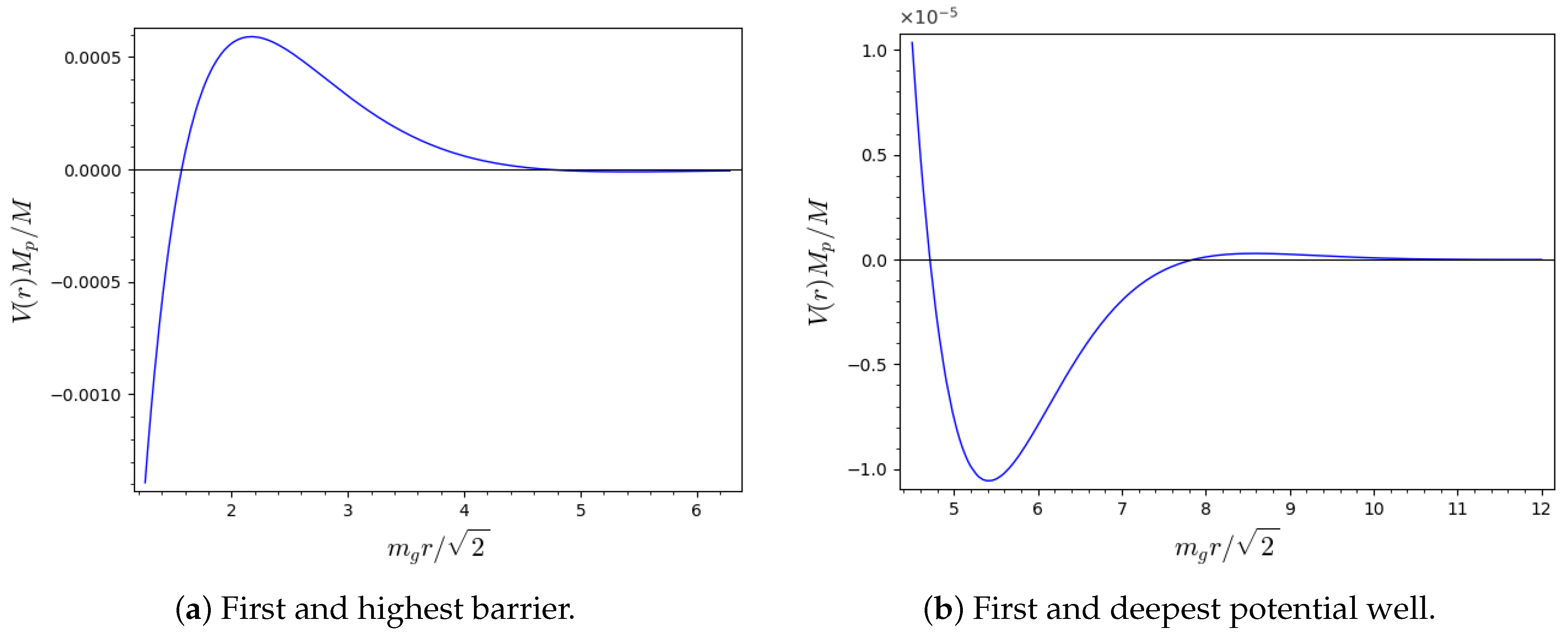
At the first and highest barrier $r_0\sim 3.1m_g^{-1}$, the potential height is given by (see Figure 1a)

$$V\left(r_0\right)\sim 4.2\times {10}^{-3}{\displaystyle \frac{M{m}_g}{M_p}}.$$

(68)

If there is enough energy to overcome this barrier, the system alternates between regions of attractive and repulsive gravity as the distance increases. The system could get trapped between two consecutive barriers, thus forming a gravitational bound state should its energy be smaller than the potential well (see Figure 1b). This effect, however, is rapidly weakened by the exponential suppression in Equation (65). Even at the deepest well depicted in Figure 1b, the existing energy from surrounding astrophysical events is likely enough to keep such bound states from forming. On the other hand, should the energy be smaller than Equation (68), the system would not collapse as the distance decreases, thus resolving the singularity at $r=0$. Note that the ratio $m_g/M_p$ is utterly negligible in Equation (68); thus, only very massive objects, such as black holes, could prevent such a collapse from happening.

6. Conclusions

Understanding the quantum nature of gravity requires, among other things, grasping the graviton kinematics and dynamics. Quantum corrections trigger new graviton self-interactions, which affect the graviton dynamics. As in any gauge theory, it is generally believed that the diffeomorphism invariance precludes the appearance of mass terms in the effective action of general relativity. However, this follows by side-stepping the non-trivial Jacobian that shows up in the path integral when diffeomorphisms (or, more generally, field redefinitions) are performed. A proper regularization of the Jacobian shows that it cannot be simply ignored.

A diffeomorphism-invariant functional measure thus requires the factor $\sqrt{\mathrm{Det}{G}_{ij}}$ to cancel out the functional Jacobian, in very much the same way that $\sqrt{-g}$ is needed for integrations in curved spacetimes. This additional factor contributes as a quantum effective potential for the graviton, giving it a mass in the linear regime. Therefore, general covariance is actually the reason for the existence, rather than for the absence, as commonly thought, of a mass for the graviton.

We stress that such a mass is not obtained by modifying general relativity. One is simply quantizing general relativity by properly considering the geometry of configuration space, which is reflected in the definition of the functional measure. One can view different configuration-space metrics as different quantization approaches to the same classical theory. The naive approach, where the functional Jacobian is disregarded, corresponds to a flat configuration space. Unfortunately, there is no known physical principle other than symmetry to help us determine the configuration-space metric. On symmetry grounds, the lowest-order configuration-space metric is curved and depends on the spacetime metric. This situation is dramatically different for Yang–Mills fields, where the lowest-order configuration-space metric is trivial and no gauge-invariant higher-order term exists. Therefore, gauge invariance manifests itself quite differently in gravity than in the other interactions, being solely responsible for keeping Yang–Mills fields massless (in the unbroken vacuum) and the graviton massive.