
Extraction of Physical Parameters of RRab Variables Using Neural Network Based Interpolator

 , ,
, ,  , ,
, ,
Abstract
1. Introduction
2. Data and Theoretical Grid
2.1. Synthetic Grid Construction
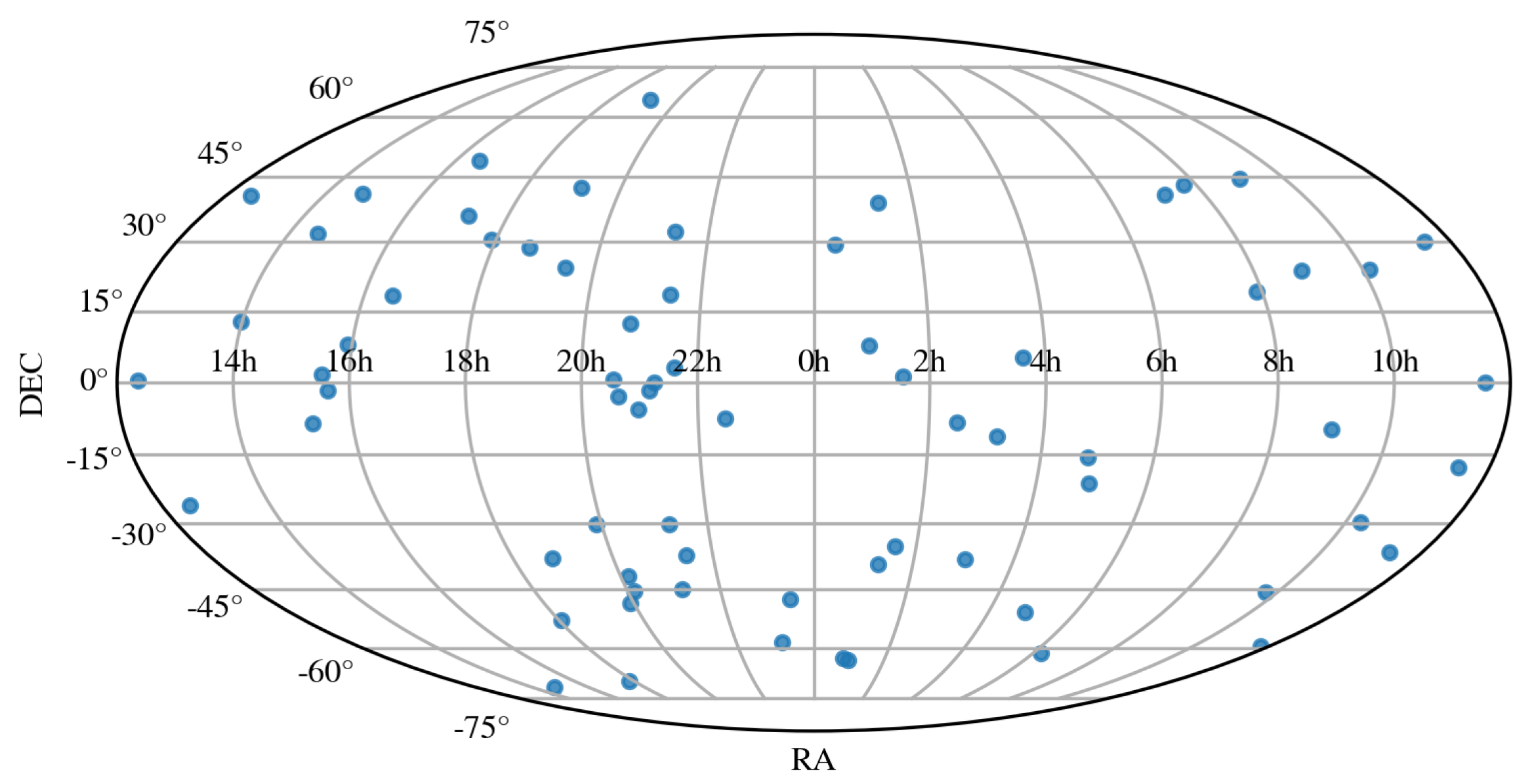
2.2. Observational TESS Sample
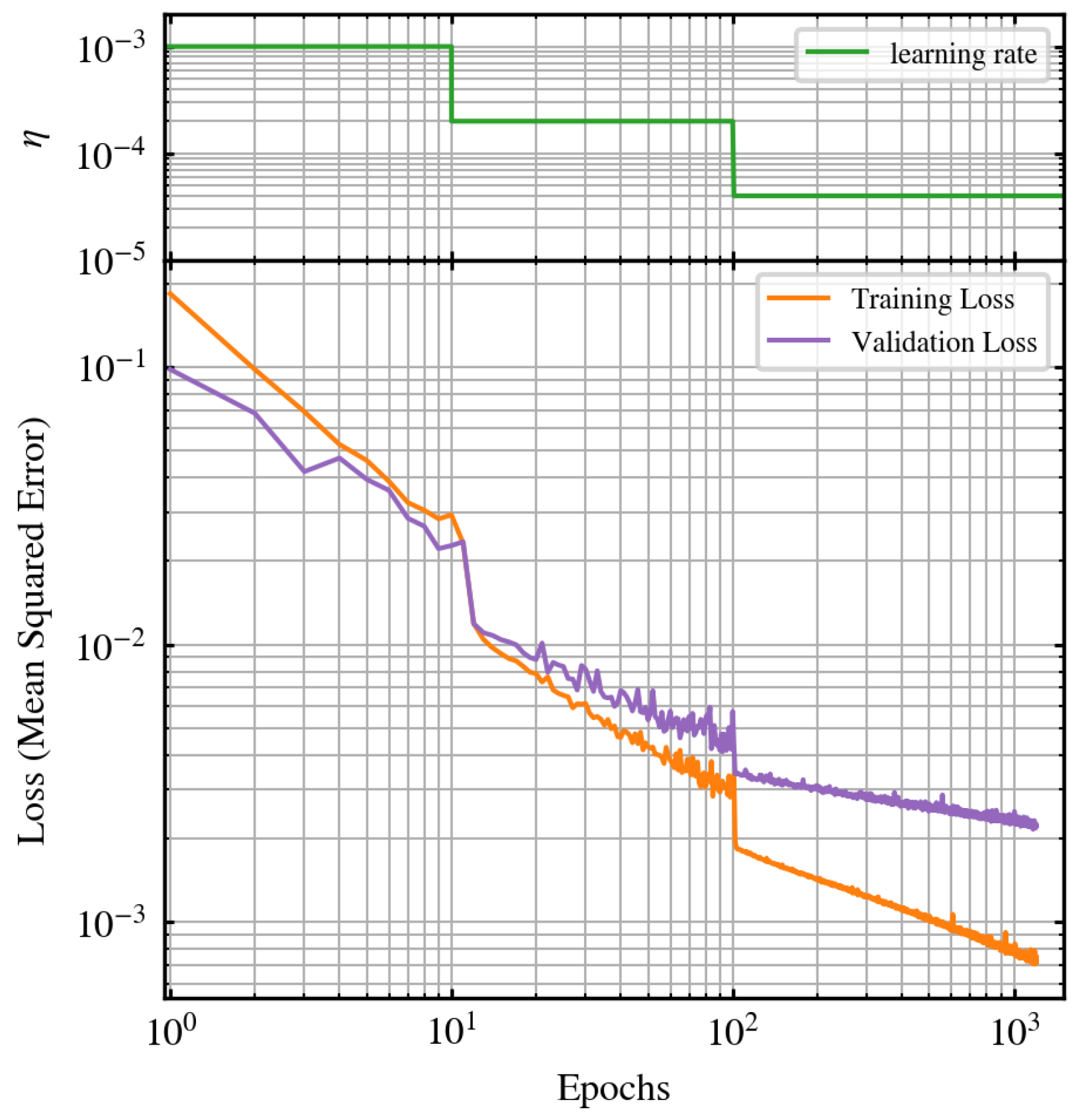
3. Parameter Estimator ANN Model
4. Results
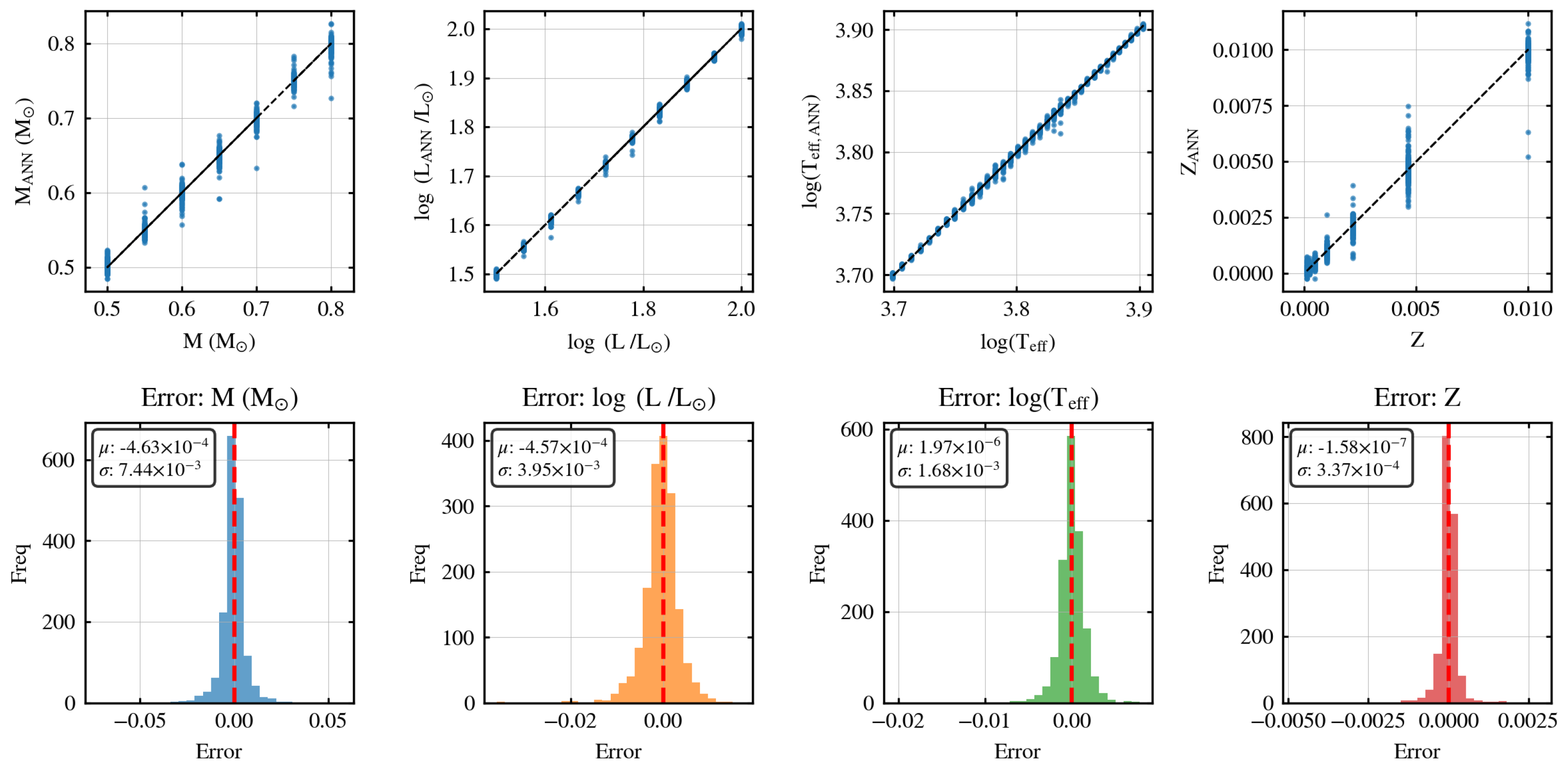
4.1. Self Inversion
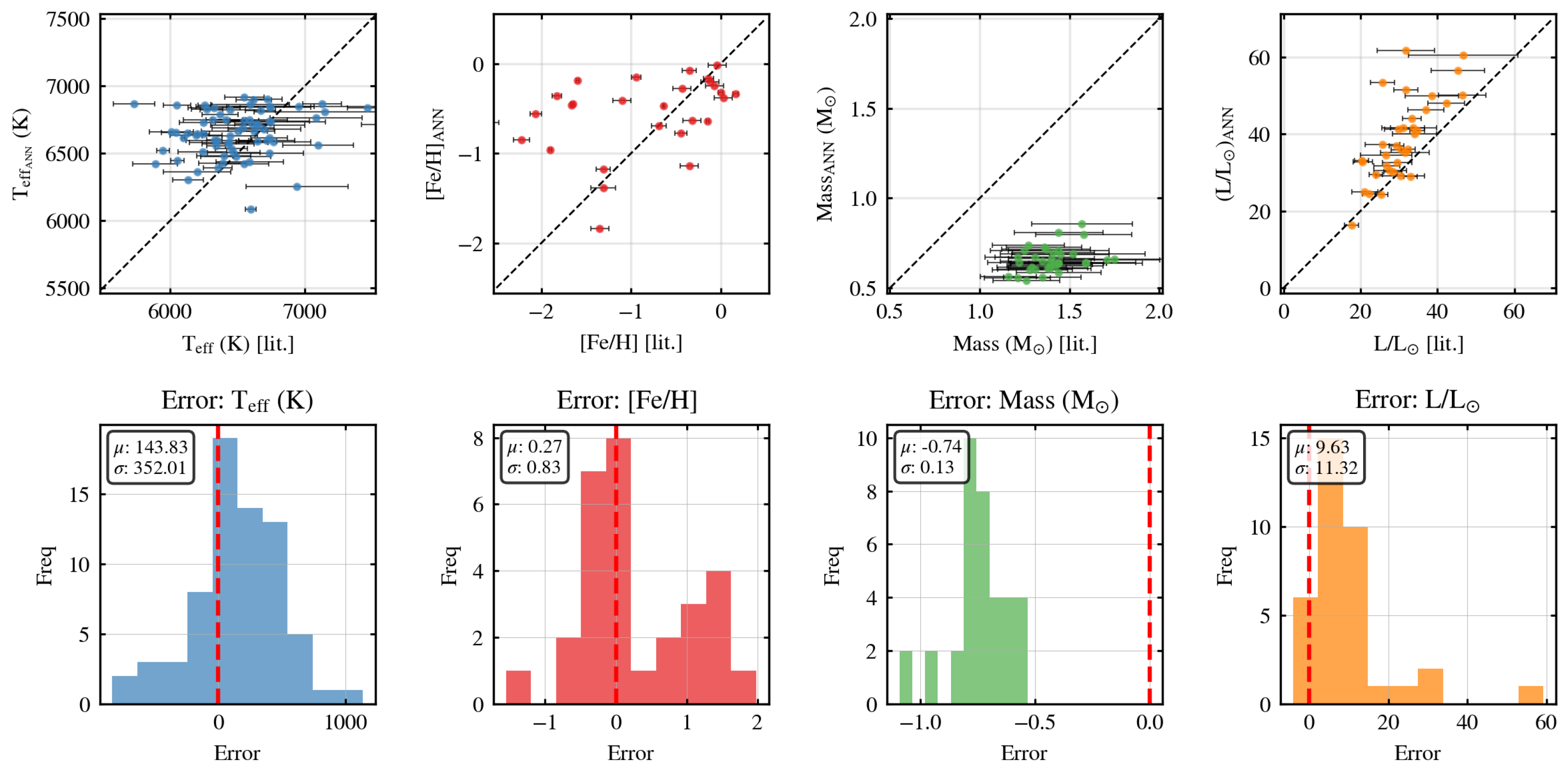
4.2. Application to TESS RRab Stars
4.2.1. Light-Curve Processing and Folding
4.2.2. Photometric Corrections and Calibration
4.2.3. ANN-Based Parameter Inference
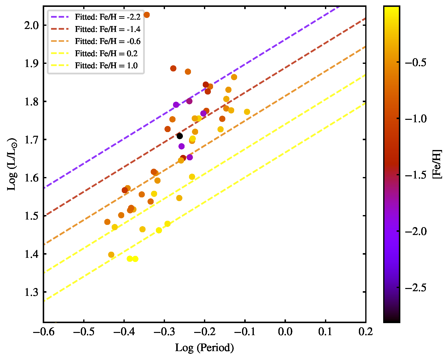
4.3. Period–Luminosity–Metallicity (PLZ) Relation
5. Conclusions
Author Contributions
Funding
Institutional Review Board Statement
Data Availability Statement
Acknowledgments
Conflicts of Interest
Abbreviations
| ANN | artificial neural network |
| PLZ | period–luminosity–metallicity (relation) |
| TESS | Transiting Exoplanet Survey Satellite |
| 1 | The RRab interpolator for generating RRab light curves for a given combination of physical parameters is publicly available at https://ann-interpolator.web.app/ (accessed on 22 June 2025). |
| 2 | https://lightkurve.github.io/lightkurve/ (accessed on 22 June 2025). |
| 3 | |
| 4 | See note 3 above. |
References
- Savino, A.; Koch, A.; Prudil, Z.; Kunder, A.; Smolec, R. The age of the Milky Way inner stellar spheroid from RR Lyrae population synthesis. Astron. Astrophys. 2020, 641, A96. [Google Scholar] [CrossRef]
- Longmore, A.J.; Fernley, J.A.; Jameson, R.F. RR Lyrae stars in globular clusters: Better distances from infrared measurements? Mon. Not. R. Astron. Soc. 1986, 220, 279–287. [Google Scholar] [CrossRef]
- Bono, G.; Caputo, F.; Castellani, V.; Marconi, M.; Storm, J. Theoretical insights into the RR Lyrae K-band period-luminosity relation. Mon. Not. R. Astron. Soc. 2001, 326, 1183–1190. [Google Scholar] [CrossRef]
- Catelan, M.; Pritzl, B.J.; Smith, H.A. The RR Lyrae Period-Luminosity Relation. I. Theoretical Calibration. Astrophys. J. Suppl. Ser. 2004, 154, 633–649. [Google Scholar] [CrossRef]
- Sollima, A.; Cacciari, C.; Valenti, E. The RR Lyrae period-K-luminosity relation for globular clusters: An observational approach. Mon. Not. R. Astron. Soc. 2006, 372, 1675–1680. [Google Scholar] [CrossRef]
- Muraveva, T.; Palmer, M.; Clementini, G.; Luri, X.; Cioni, M.R.L.; Moretti, M.I.; Marconi, M.; Ripepi, V.; Rubele, S. New Near-infrared Period-Luminosity-Metallicity Relations for RR Lyrae Stars and the Outlook for Gaia. Astrophys. J. 2015, 807, 127. [Google Scholar] [CrossRef]
- Bhardwaj, A.; Rejkuba, M.; de Grijs, R.; Yang, S.C.; Herczeg, G.J.; Marconi, M.; Singh, H.P.; Kanbur, S.; Ngeow, C.C. RR Lyrae Variables in Messier 53: Near-infrared Period-Luminosity Relations and the Calibration Using Gaia Early Data Release 3. Astron. J. 2021, 909, 200. [Google Scholar] [CrossRef]
- Beaton, R.L.; Freedman, W.L.; Madore, B.F.; Bono, G.; Carlson, E.K.; Clementini, G.; Durbin, M.J.; Garofalo, A.; Hatt, D.; Jang, I.S.; et al. The Carnegie-Chicago Hubble Program. I. An Independent Approach to the Extragalactic Distance Scale Using Only Population II Distance Indicators. Astrophys. J. 2016, 832, 210. [Google Scholar] [CrossRef]
- Bhardwaj, A. High-precision distance measurements with classical pulsating stars. J. Astrophys. Astron. 2020, 41, 23. [Google Scholar] [CrossRef]
- Catelan, M. Horizontal branch stars: The interplay between observations and theory, and insights into the formation of the Galaxy. Astrophys. Space Sci. 2009, 320, 261–309. [Google Scholar] [CrossRef]
- Kunder, A.; Valenti, E.; Dall’Ora, M.; Pietrukowicz, P.; Sneden, C.; Bono, G.; Braga, V.F.; Ferraro, I.; Fiorentino, G.; Iannicola, G.; et al. Impact of Distance Determinations on Galactic Structure. II. Old Tracers. Space Sci. Rev. 2018, 214, 90. [Google Scholar] [CrossRef]
- Cacciari, C.; Corwin, T.M.; Carney, B.W. A Multicolor and Fourier Study of RR Lyrae Variables in the Globular Cluster NGC 5272 (M3). Astron. J. 2005, 129, 267–302. [Google Scholar] [CrossRef]
- Deb, S.; Singh, H.P. Physical parameters of the Small Magellanic Cloud RR Lyrae stars and the distance scale. Mon. Not. R. Astron. Soc. 2010, 402, 691–704. [Google Scholar] [CrossRef]
- Nemec, J.M.; Smolec, R.; Benkő, J.M.; Moskalik, P.; Kolenberg, K.; Szabó, R.; Kurtz, D.W.; Bryson, S.; Guggenberger, E.; Chadid, M.; et al. Fourier analysis of non-Blazhko ab-type RR Lyrae stars observed with the Kepler space telescope. Mon. Not. R. Astron. Soc. 2011, 417, 1022–1053. [Google Scholar] [CrossRef]
- Marconi, M.; Coppola, G.; Bono, G.; Braga, V.; Pietrinferni, A.; Buonanno, R.; Castellani, M.; Musella, I.; Ripepi, V.; Stellingwerf, R.F. On a New Theoretical Framework for RR Lyrae Stars. I. The Metallicity Dependence. Astrophys. J. 2015, 808, 50. [Google Scholar] [CrossRef]
- De Somma, G.; Marconi, M.; Molinaro, R.; Cignoni, M.; Musella, I.; Ripepi, V. An Extended Theoretical Scenario for Classical Cepheids. I. Modeling Galactic Cepheids in the Gaia Photometric System. Astron. J. Suppl. Ser. 2020, 247, 30. [Google Scholar] [CrossRef]
- De Somma, G.; Marconi, M.; Molinaro, R.; Ripepi, V.; Leccia, S.; Musella, I. An Updated Metal-dependent Theoretical Scenario for Classical Cepheids. Astrophys. J. Suppl. Ser. 2022, 262, 25. [Google Scholar] [CrossRef]
- Smolec, R.; Moskalik, P. Convective Hydrocodes for Radial Stellar Pulsation. Physical and Numerical Formulation. Acta Astron. 2008, 58, 193–232. [Google Scholar] [CrossRef]
- Paxton, B.; Bildsten, L.; Dotter, A.; Herwig, F.; Lesaffre, P.; Timmes, F. Modules for Experiments in Stellar Astrophysics (MESA). Astrophys. J. Suppl. Ser. 2011, 192, 3. [Google Scholar] [CrossRef]
- Paxton, B.; Cantiello, M.; Arras, P.; Bildsten, L.; Brown, E.F.; Dotter, A.; Mankovich, C.; Montgomery, M.H.; Stello, D.; Timmes, F.X.; et al. Modules for Experiments in Stellar Astrophysics (MESA): Planets, Oscillations, Rotation, and Massive Stars. Astrophys. J. Suppl. Ser. 2013, 208, 4. [Google Scholar] [CrossRef]
- Paxton, B.; Marchant, P.; Schwab, J.; Bauer, E.B.; Bildsten, L.; Cantiello, M.; Dessart, L.; Farmer, R.; Hu, H.; Langer, N.; et al. Modules for Experiments in Stellar Astrophysics (MESA): Binaries, Pulsations, and Explosions. Astrophys. J. Suppl. Ser. 2015, 220, 15. [Google Scholar] [CrossRef]
- Paxton, B.; Schwab, J.; Bauer, E.B.; Bildsten, L.; Blinnikov, S.; Duffell, P.; Farmer, R.; Goldberg, J.A.; Marchant, P.; Sorokina, E.; et al. Modules for Experiments in Stellar Astrophysics (MESA): Convective Boundaries, Element Diffusion, and Massive Star Explosions. Astrophys. J. Suppl. Ser. 2018, 234, 34. [Google Scholar] [CrossRef]
- Paxton, B.; Smolec, R.; Schwab, J.; Gautschy, A.; Bildsten, L.; Cantiello, M.; Dotter, A.; Farmer, R.; Goldberg, J.A.; Jermyn, A.S.; et al. Modules for Experiments in Stellar Astrophysics (MESA): Pulsating Variable Stars, Rotation, Convective Boundaries, and Energy Conservation. Astrophys. J. Suppl. Ser. 2019, 243, 10. [Google Scholar] [CrossRef]
- Torres, G.; Andersen, J.; Giménez, A. Accurate masses and radii of normal stars: Modern results and applications. Astron. Astrophys. Rev. 2010, 18, 67–126. [Google Scholar] [CrossRef]
- Southworth, J. DEBCat: A Catalog of Detached Eclipsing Binary Stars. In Proceedings of the Living Together: Planets, Host Stars and Binaries, Litomyšl, Czech Republic, 8–12 September 2014; Rucinski, S.M., Torres, G., Zejda, M., Eds.; Astronomical Society of the Pacific Conference Series; Astronomical Society of the Pacific: San Francisco, CA, USA, 2015; Volume 496, p. 164. [Google Scholar] [CrossRef]
- Grison, P.; Beaulieu, J.P.; Pritchard, J.D.; Tobin, W.; Ferlet, R.; Vidal-Madjar, A.; Guibert, J.; Alard, C.; Moreau, O.; Tajahmady, F.; et al. EROS catalogue of eclipsing binary stars in the bar of the Large Magellanic Cloud. Astron. Astrophys. Suppl. 1995, 109, 447–469. [Google Scholar]
- Alcock, C.; Allsman, R.A.; Alves, D.R.; Axelrod, T.S.; Becker, A.C.; Basu, A.; Baskett, L.; Bennett, D.P.; Cook, K.H.; Freeman, K.C.; et al. The RR Lyrae Population of the Galactic Bulge from the MACHO Database: Mean Colors and Magnitudes. Astrophys. J. 1998, 492, 190–199. [Google Scholar] [CrossRef]
- Rucinski, S.M.; Maceroni, C. Eclipsing Binaries in the OGLE Variable Star Catalogs. V. Long-Period EB-Type Light Curve Systems in the Small Magellanic Cloud and the PLC-βRelation. Astron. J. 2001, 121, 254–266. [Google Scholar] [CrossRef]
- Pojmanski, G. The All Sky Automated Survey. Catalog of Variable Stars. I. 0 h–6 hQuarter of the Southern Hemisphere. Acta Astron. 2002, 52, 397–427. [Google Scholar] [CrossRef]
- Alonso, R.; Brown, T.M.; Torres, G.; Latham, D.W.; Sozzetti, A.; Mandushev, G.; Belmonte, J.A.; Charbonneau, D.; Deeg, H.J.; Dunham, E.W.; et al. TrES-1: The Transiting Planet of a Bright K0 V Star. Astrophys. J. Lett. 2004, 613, L153–L156. [Google Scholar] [CrossRef]
- Bakos, G.; Noyes, R.W.; Kovács, G.; Stanek, K.Z.; Sasselov, D.D.; Domsa, I. Wide-Field Millimagnitude Photometry with the HAT: A Tool for Extrasolar Planet Detection. Publ. Astron. Soc. Pac. 2004, 116, 266–277. [Google Scholar] [CrossRef]
- Loeillet, B.; Bouchy, F.; Deleuil, M.; Royer, F.; Bouret, J.C.; Moutou, C.; Barge, P.; de Laverny, P.; Pont, F.; Recio-Blanco, A.; et al. Doppler search for exoplanet candidates and binary stars in a CoRoT field using a multi-fiber spectrograph. I. Global analysis and first results. Astron. Astrophys. 2008, 479, 865–875. [Google Scholar] [CrossRef]
- Matijevič, G.; Prša, A.; Orosz, J.A.; Welsh, W.F.; Bloemen, S.; Barclay, T. Kepler Eclipsing Binary Stars. III. Classification of Kepler Eclipsing Binary Light Curves with Locally Linear Embedding. Astron. J. 2012, 143, 123. [Google Scholar] [CrossRef]
- Das, S.; Bhardwaj, A.; Kanbur, S.M.; Singh, H.P.; Marconi, M. On the variation of light-curve parameters of RR Lyrae variables at multiple wavelengths. Mon. Not. R. Astron. Soc. 2018, 481, 2000–2017. [Google Scholar] [CrossRef]
- Kumar, N.; Prugniel, P.; Singh, H.P. Physical parameters of stars in NGC 6397 using ANN-based interpolation and full spectrum fitting. New Astron. 2025, 119, 102416. [Google Scholar] [CrossRef]
- Bellinger, E.P.; Angelou, G.C.; Hekker, S.; Basu, S.; Ball, W.H.; Guggenberger, E. Fundamental Parameters of Main-Sequence Stars in an Instant with Machine Learning. Astrophys. J. 2016, 830, 31. [Google Scholar] [CrossRef]
- Kumar, N.; Bhardwaj, A.; Singh, H.P.; Das, S.; Marconi, M.; Kanbur, S.M.; Prugniel, P. Predicting light curves of RR Lyrae variables using artificial neural network based interpolation of a grid of pulsation models. Mon. Not. R. Astron. Soc. 2023, 522, 1504–1520. [Google Scholar] [CrossRef]
- Bellinger, E.P.; Kanbur, S.M.; Bhardwaj, A.; Marconi, M. When a period is not a full stop: Light-curve structure reveals fundamental parameters of Cepheid and RR Lyrae stars. Mon. Not. R. Astron. Soc. 2020, 491, 4752–4767. [Google Scholar] [CrossRef]
- Kumar, N.; Bhardwaj, A.; Singh, H.P.; Rejkuba, M.; Marconi, M.; Prugniel, P. Multiwavelength photometric study of RR lyrae variables in the globular cluster NGC 5272 (Messier 3). Mon. Not. R. Astron. Soc. 2024, 531, 2976–2997. [Google Scholar] [CrossRef]
- van Albada, T.S.; Baker, N. On the Masses, Luminosities, and Compositions of Horizontal-Branch Stars. Astrophys. J. 1971, 169, 311. [Google Scholar] [CrossRef]
- Ricker, G.R.; Winn, J.N.; Vanderspek, R.; Latham, D.W.; Bakos, G.A.; Bean, J.L.; Berta-Thompson, Z.K.; Brown, T.M.; Buchhave, L.; Butler, N.R.; et al. Transiting Exoplanet Survey Satellite (TESS). J. Astron. Telesc. Instrum. Syst. 2015, 1, 014003. [Google Scholar] [CrossRef]
- Molnár, L.; Bódi, A.; Pál, A.; Bhardwaj, A.; Hambsch, F.; Benkő, J.M.; Derekas, A.; Ebadi, M.; Joyce, M.; Hasanzadeh, A.; et al. First Results on RR Lyrae Stars with the TESS Space Telescope: Untangling the Connections between Mode Content, Colors, and Distances. Astrophys. J. Suppl. Ser. 2021, 258, 8. [Google Scholar] [CrossRef]
- Stassun, K.G.; Oelkers, R.J.; Pepper, J.; Paegert, M.; De Lee, N.; Torres, G.; Latham, D.W.; Charpinet, S.; Dressing, C.D.; Huber, D.; et al. The TESS Input Catalog and Candidate Target List. Astron. J. 2018, 156, 102. [Google Scholar] [CrossRef]
- Paegert, M.; Stassun, K.G.; Collins, K.A.; Pepper, J.; Torres, G.; Jenkins, J.; Twicken, J.D.; Latham, D.W. TESS Input Catalog versions 8.1 and 8.2: Phantoms in the 8.0 Catalog and How to Handle Them. arXiv 2021, arXiv:2108.04778. [Google Scholar]
- Stassun, K.G.; Oelkers, R.J.; Paegert, M.; Torres, G.; Pepper, J.; De Lee, N.; Collins, K.; Latham, D.W.; Muirhead, P.S.; Chittidi, J.; et al. The Revised TESS Input Catalog and Candidate Target List. Astron. J. 2019, 158, 138. [Google Scholar] [CrossRef]
- Lightkurve Collaboration; Cardoso, J.V.d.M.; Hedges, C.; Gully-Santiago, M.; Saunders, N.; Cody, A.M.; Barclay, T.; Hall, O.; Sagear, S.; Turtelboom, E.; et al. Lightkurve: Kepler and TESS Time Series Analysis in Python; Astrophysics Source Code Library. 2018. Available online: https://ui.adsabs.harvard.edu/abs/2018ascl.soft12013L/abstract (accessed on 15 June 2025).
- Cybenko, G. Approximation by superpositions of a sigmoidal function. Math. Control Signals Syst. 1989, 2, 303–314. [Google Scholar] [CrossRef]
- Hornik, K.; Stinchcombe, M.; White, H. Multilayer feedforward networks are universal approximators. Neural Netw. 1989, 2, 359–366. [Google Scholar] [CrossRef]
- Hornik, K. Approximation capabilities of multilayer feedforward networks. Neural Netw. 1991, 4, 251–257. [Google Scholar] [CrossRef]
- Kingma, D.P.; Ba, J. Adam: A Method for Stochastic Optimization. arXiv 2014, arXiv:1412.6980. [Google Scholar]
- Jenkins, J.M.; Twicken, J.D.; McCauliff, S.; Campbell, J.; Sanderfer, D.; Lung, D.; Mansouri-Samani, M.; Girouard, F.; Tenenbaum, P.; Klaus, T.; et al. The TESS science processing operations center. In Proceedings of the Software and Cyberinfrastructure for Astronomy IV, Edinburgh, UK, 17–21 July 2016; Chiozzi, G., Guzman, J.C., Eds.; Society of Photo-Optical Instrumentation Engineers (SPIE) Conference Series; SPIE: Bellingham, WA, USA, 2016; Volume 9913, p. 99133E. [Google Scholar] [CrossRef]
- Lomb, N.R. Least-squares frequency analysis of unequally spaced data. Astrophys. Space Sci. 1976, 39, 447–462. [Google Scholar] [CrossRef]
- Scargle, J.D. Studies in astronomical time series analysis. II. Statistical aspects of spectral analysis of unevenly spaced data. Astrophys. J. 1982, 263, 835–853. [Google Scholar] [CrossRef]
- Schlafly, E.F.; Finkbeiner, D.P. Measuring Reddening with Sloan Digital Sky Survey Stellar Spectra and Recalibrating SFD. Astrophys. J. 2011, 737, 103. [Google Scholar] [CrossRef]
- Piersanti, L.; Straniero, O.; Cristallo, S. A method to derive the absolute composition of the Sun, the solar system, and the stars*. Astron. Astrophys. 2007, 462, 1051–1062. [Google Scholar] [CrossRef]
- Asplund, M.; Grevesse, N.; Sauval, A.J. The Solar Chemical Composition. ASPC Conf. 2005, 336, 25. [Google Scholar] [CrossRef]
- Marconi, M.; Minniti, D. Gauging the Helium Abundance of the Galactic Bulge RR Lyrae Stars. Astrophys. J. Lett. 2018, 853, L20. [Google Scholar] [CrossRef]


| Parameter | Range | Step Size |
|---|---|---|
| Mass () | 0.5–0.8 | 0.05 |
| 1.50–2.00 | 0.0555 | |
| (K) | 5000–8000 | 88.23 |
| Metallicity (Z) | – | logarithmic steps |
| Hydrogen fraction (X) | 0.755–0.745 | computed as |
| Hyperparameter | Values |
|---|---|
| Number of layers | 1 to 6 |
| Units per layer | 16, 32, 64, 128, 256, 512 |
| Activation function | ReLU, tanh |
| Learning rate | to (log-uniform sampling) |
| Batch size | 32 (fixed) |
| Optimizer | adam [50] |
| Kernel initializer | Glorot Uniform (fixed seed) |
| Loss function | Mean Squared Error (MSE) |
| Parameter | MSE | Relative RMSE (%) |
|---|---|---|
| Mass (M) | 1.15 | |
| Luminosity (L) | 0.23 | |
| 0.04 | ||
| Metallicity (Z) | 12.81 |
| ID | TESS ID | Plxlit | Period | Period LS | Mlit | MANN | Lumlit | LumANN | [Fe/H]lit | [Fe/H]ANN | logglit | ||
|---|---|---|---|---|---|---|---|---|---|---|---|---|---|
| (”) | (d) | (d) | (K) | (K) | (M⊙) | (M⊙) | (LM⊙) | (LM⊙) | (dex) | (dex) | (dex) | ||
| XZ Dra | 229913521 | 1.30 ± 0.02 | 0.476475 | 0.476574 | 6447 ± 224 | 6824 | 1.31 ± 0.22 | 0.67 | 34.76 ± 1.98 | 40.91 | – | −0.56 | 3.21 ± 0.12 |
| V1195 Her | 232570970 | 0.53 ± 0.02 | 0.609729 | 0.608373 | 5889 ± 167 | 6420 | – | 0.67 | – | 56.91 | −1.60 ± 0.01 | −0.19 | – |
| TW Lyn | 241174387 | 0.62 ± 0.04 | 0.481854 | 0.481025 | 6008 ± 162 | 6659 | – | 0.62 | – | 39.10 | −0.64 ± 0.01 | −0.47 | – |
| TT Lyn | 29172806 | 1.22 ± 0.04 | 0.597443 | 0.597684 | 6191 ± 193 | 6635 | – | 0.65 | – | 52.51 | −1.65 ± 0.02 | −0.45 | – |
| TW Boo | 68076619 | 0.72 ± 0.02 | 0.532264 | 0.531162 | 6247 ± 42 | 6645 | – | 0.70 | – | 45.32 | −1.46 ± 0.07 | – | – |
| SV Eri | 9843991 | 1.22 ± 0.06 | 0.713900 | 0.713374 | 6200 ± 249 | 6360 | – | 0.81 | – | 60.43 | −2.06 ± 0.06 | −0.56 | – |
| SS Tau | 311091712 | 0.67 ± 0.05 | 0.369910 | 0.369768 | 6724 ± 108 | 6903 | 1.43 ± 0.26 | 0.64 | 21.14 ± 3.31 | 25.00 | 0.17 ± 0.03 | −0.33 | 3.53 ± 0.11 |
| RX Eri | 114923989 | 1.62 ± 0.03 | 0.587252 | 0.586150 | 6443 ± 205 | 6629 | – | 0.63 | – | 49.70 | – | −0.56 | – |
| U Lep | 146324929 | 0.93 ± 0.03 | 0.581458 | 0.580807 | 6541 ± 229 | 6689 | – | 0.74 | – | 58.66 | – | – | – |
| TZ Aur | 328588068 | 0.66 ± 0.04 | 0.391673 | 0.391437 | 7128 ± 145 | 6867 | 1.59 ± 0.28 | 0.64 | 26.79 ± 3.39 | 31.72 | −0.15 ± 0.02 | −0.64 | 3.58 ± 0.10 |
| SZ Gem | 63172763 | 0.59 ± 0.04 | 0.501165 | 0.501342 | 6050 ± 101 | 6856 | – | 0.71 | – | 42.36 | −1.65 ± 0.13 | – | – |
| EZ Cnc | 197217727 | 0.50 ± 0.05 | 0.545777 | 0.546779 | 6625 ± 100 | 6662 | 1.39 ± 0.23 | 0.61 | 31.60 ± 6.34 | 35.19 | −0.00 ± 0.03 | −0.32 | 3.32 ± 0.13 |
| SS Gru | 129710422 | 0.14 ± 0.04 | 0.959791 | 0.956326 | 6942 ± 379 | 6252 | – | 0.95 | – | 291.22 | – | −0.56 | – |
| VW Scl | 41833926 | 0.85 ± 0.07 | 0.510917 | 0.511665 | 6672 ± 111 | 6816 | 1.41 ± 0.23 | 0.70 | 31.06 ± 5.55 | 41.71 | −1.27 ± 0.05 | – | 3.35 ± 0.11 |
| Z Mic | 89358641 | 0.81 ± 0.07 | 0.586928 | 0.585981 | 6398 ± 200 | 6480 | 1.28 ± 0.21 | 0.60 | 34.01 ± 5.69 | 40.01 | – | −0.18 | 3.19 ± 0.13 |
| VX Scl | 32282599 | 0.43 ± 0.03 | 0.637078 | 0.635441 | 6716 ± 208 | 6597 | – | 0.76 | – | 59.59 | – | −0.95 | – |
| RZ Cet | 1129237 | 0.68 ± 0.04 | 0.510600 | 0.511475 | 6248 ± 182 | 6729 | 1.21 ± 0.18 | 0.67 | 25.68 ± 3.12 | 53.38 | −1.90 ± 0.02 | −0.96 | 3.25 ± 0.12 |
| BN Aqr | 39999072 | 0.38 ± 0.06 | 0.469600 | 0.468717 | 6955 ± 760 | 6849 | 1.52 ± 0.40 | 0.69 | 46.69 ± 14.23 | 60.60 | – | – | 3.27 ± 0.31 |
| CP Aqr | 248483300 | 0.78 ± 0.09 | 0.463400 | 0.463006 | 7148 ± 522 | 6806 | 1.59 ± 0.32 | 0.64 | 26.65 ± 6.66 | 34.45 | – | −0.74 | 3.59 ± 0.22 |
| SW Aqr | 387498678 | 0.76 ± 0.23 | 0.459305 | 0.459871 | – | 6824 | – | 0.72 | – | 43.47 | – | – | – |
| RR Cet | 344299442 | 1.52 ± 0.08 | 0.553041 | 0.552368 | 6650 ± 139 | 6589 | 1.40 ± 0.24 | 0.66 | 42.32 ± 4.75 | 48.09 | −1.35 ± 0.10 | −1.84 | 3.20 ± 0.10 |
| SX Aqr | 353029655 | 0.62 ± 0.07 | 0.535708 | 0.536120 | 6325 ± 194 | 6838 | 1.25 ± 0.19 | 0.71 | 31.85 ± 7.46 | 61.80 | – | −1.84 | 3.19 ± 0.14 |
| AO Peg | 283289876 | 0.35 ± 0.04 | 0.547245 | 0.546917 | 6342 ± 71 | 6554 | – | 0.67 | – | 51.16 | −1.25 ± 0.07 | −2.81 | – |
| SW And | 437761208 | 1.78 ± 0.16 | 0.442261 | 0.441881 | 6735 ± 138 | 6613 | 1.44 ± 0.24 | 0.59 | 30.35 ± 6.28 | 29.13 | −0.07 ± 0.10 | −0.25 | 3.38 ± 0.13 |
| DM Cyg | 117638854 | 0.97 ± 0.05 | 0.419868 | 0.419951 | 6415 ± 151 | 6748 | 1.29 ± 0.19 | 0.61 | 20.62 ± 2.50 | 32.85 | 0.03 ± 0.10 | −0.38 | 3.42 ± 0.10 |
| XX And | 186452465 | 0.69 ± 0.05 | 0.722772 | 0.721256 | 6097 ± 9 | 6613 | – | 0.70 | – | 67.68 | −1.67 ± 0.01 | −0.46 | – |
| DH Hya | 47291018 | 0.47 ± 0.04 | 0.488996 | 0.488922 | 6259 ± 54 | 6856 | – | 0.71 | – | 59.94 | −1.52 ± 0.09 | – | – |
| RR Leo | 3941985 | 1.00 ± 0.09 | 0.452403 | 0.451699 | 6593 ± 291 | 6863 | 1.37 ± 0.25 | 0.72 | 33.79 ± 6.00 | 41.59 | – | – | 3.28 ± 0.16 |
| WY Ant | 168276785 | 0.91 ± 0.06 | 0.574350 | 0.575440 | 6765 ± 277 | 6583 | 1.45 ± 0.27 | 0.69 | 46.47 ± 6.23 | 50.15 | – | – | 3.21 ± 0.15 |
| V595 Cen | 152231997 | 0.44 ± 0.03 | 0.690994 | 0.691325 | 6430 ± 191 | 6569 | – | 0.65 | – | 53.30 | – | −0.25 | – |
| TU UMa | 144376546 | 1.56 ± 0.06 | 0.557658 | 0.556678 | 6200 ± 65 | 6643 | – | 0.65 | – | 44.82 | −1.31 ± 0.14 | −1.39 | – |
| SS Leo | 49417864 | 1.13 ± 0.72 | 0.626351 | 0.626993 | – | 6676 | – | 0.70 | – | 58.65 | – | −1.80 | – |
| W Crt | 219249305 | 0.75 ± 0.04 | 0.412012 | 0.412036 | 6740 ± 305 | 6845 | 1.44 ± 0.27 | 0.64 | 29.59 ± 3.80 | 32.68 | – | −0.70 | 3.39 ± 0.15 |
| UV Vir | 377172421 | 0.56 ± 0.05 | 0.587065 | 0.586541 | 7550 ± 130 | 6714 | 1.75 ± 0.28 | 0.66 | 38.59 ± 6.88 | 49.96 | −1.10 ± 0.10 | −0.41 | 3.56 ± 0.11 |
| UZ CVn | 376689735 | 0.51 ± 0.03 | 0.697793 | 0.696838 | 6329 ± 58 | 6599 | – | 0.66 | – | 56.78 | −2.22 ± 0.09 | −0.85 | – |
| SV Hya | 453469791 | 1.21 ± 0.05 | 0.478527 | 0.478892 | 6744 ± 324 | 6850 | 1.44 ± 0.28 | 0.71 | 31.79 ± 3.08 | 51.43 | – | – | 3.36 ± 0.15 |
| UY Boo | 458457951 | 0.62 ± 0.05 | 0.650800 | 0.651139 | 6433 ± 292 | 6581 | – | 0.77 | – | 69.01 | – | -0.73 | – |
| RS Boo | 409373422 | 1.36 ± 0.04 | 0.377365 | 0.377471 | 6610 ± 132 | 6719 | 1.38 ± 0.22 | 0.61 | 24.05 ± 1.74 | 29.52 | −0.12 ± 0.10 | −0.21 | 3.43 ± 0.09 |
| V413 CrA | 253708643 | 1.13 ± 0.05 | 0.589343 | 0.589858 | 5945 ± 47 | 6521 | – | 0.60 | – | 50.39 | −0.94 ± 0.05 | −0.15 | – |
| V4424 Sgr | 271404999 | 1.70 ± 0.04 | 0.424503 | 0.424840 | 6240 ± 181 | 6511 | 1.21 ± 0.18 | 0.55 | 25.46 ± 1.63 | 24.36 | – | −0.00 | 3.25 ± 0.10 |
| TV Lib | 79403057 | 0.79 ± 0.04 | 0.269624 | 0.269903 | 6620 ± 132 | 6897 | 1.39 ± 0.23 | 0.64 | 17.68 ± 1.81 | 16.29 | −0.43 ± 0.10 | −0.28 | 3.57 ± 0.10 |
| BT Aqr | 248815852 | 0.56 ± 0.05 | 0.406357 | 0.406222 | 6700 ± 268 | 6681 | 1.42 ± 0.27 | 0.62 | 25.69 ± 4.50 | 37.35 | – | −0.55 | 3.44 ± 0.15 |
| AA Aql | 248097218 | 0.68 ± 0.05 | 0.361768 | 0.361829 | 6550 ± 146 | 6915 | 1.35 ± 0.24 | 0.65 | 27.71 ± 4.25 | 30.46 | −0.32 ± 0.10 | −0.63 | 3.35 ± 0.12 |
| V456 Ser | 46253107 | 0.22 ± 0.04 | 0.517558 | 0.517328 | 6600 ± 40 | 6084 | – | 0.76 | – | 151.05 | −2.64 ± 0.17 | −0.66 | – |
| VY Ser | 371355048 | 1.32 ± 0.07 | 0.714096 | 0.712959 | 6055 ± 50 | 6448 | – | 0.70 | – | 64.02 | −1.82 ± 0.05 | −0.36 | – |
| V341 Aql | 375822497 | 0.84 ± 0.05 | 0.578042 | 0.579124 | 6504 ± 272 | 6666 | – | 0.73 | – | 63.17 | – | −1.63 | – |
| AT Ser | 264584937 | 0.58 ± 0.05 | 0.746609 | 0.745240 | 6591 ± 249 | 6436 | – | 0.75 | – | 73.06 | – | −0.47 | – |
| DX Del | 85211589 | 1.68 ± 0.03 | 0.472611 | 0.472674 | 6454 ± 118 | 6534 | 1.31 ± 0.21 | 0.60 | 32.36 ± 1.84 | 36.11 | −0.14 ± 0.06 | −0.16 | 3.24 ± 0.09 |
| VX Her | 356085581 | 0.98 ± 0.06 | 0.455356 | 0.456175 | 6369 ± 135 | 6786 | 1.27 ± 0.20 | 0.74 | 37.00 ± 4.74 | 46.23 | −1.45 ± 0.07 | – | 3.14 ± 0.11 |
| BN Vul | 111443222 | 1.40 ± 0.03 | 0.594132 | 0.593941 | 6318 ± 222 | 6749 | – | 0.85 | – | 143.31 | – | −0.86 | – |
| TW Her | 10581605 | 0.86 ± 0.02 | 0.399596 | 0.400107 | 7465 ± 147 | 6836 | 1.71 ± 0.29 | 0.66 | 29.37 ± 1.94 | 36.89 | −0.35 ± 0.10 | −1.14 | 3.65 ± 0.09 |
| CN Lyr | 317170031 | 1.11 ± 0.03 | 0.411382 | 0.411798 | 6355 ± 106 | 6393 | 1.26 ± 0.19 | 0.54 | 22.33 ± 1.79 | 24.38 | −0.04 ± 0.10 | −0.01 | 3.36 ± 0.09 |
| VZ Her | 85516380 | 0.63 ± 0.02 | 0.440360 | 0.440466 | 5732 ± 153 | 6870 | – | 0.71 | – | 42.43 | −1.71 ± 0.01 | – | – |
| FN Lyr | 158553034 | 0.30 ± 0.03 | 0.527390 | 0.527304 | 6745 ± 410 | 6735 | – | 0.78 | – | 77.00 | – | −1.09 | – |
| SW For | 175492625 | 0.36 ± 0.02 | 0.803760 | 0.803760 | 6389 ± 176 | 6426 | – | 0.67 | – | 59.24 | – | −0.26 | – |
| U Pic | 259590223 | 0.73 ± 0.02 | 0.440373 | 0.440466 | 6642 ± 106 | 6718 | 1.40 ± 0.23 | 0.63 | 30.57 ± 2.50 | 35.96 | −0.69 ± 0.08 | −0.69 | 3.34 ± 0.09 |
| CD Vel | 34069197 | 0.57 ± 0.03 | 0.573516 | 0.572059 | 7099 ± 261 | 6558 | 1.58 ± 0.27 | 0.80 | 54.15 ± 6.25 | 75.49 | – | −0.74 | 3.26 ± 0.12 |
| ST Pic | 150166721 | 2.00 ± 0.02 | 0.485749 | 0.486130 | 6549 ± 182 | 6422 | 1.35 ± 0.22 | 0.56 | 33.05 ± 1.70 | 28.96 | – | −0.06 | 3.27 ± 0.10 |
| AE Tuc | 234507163 | 0.63 ± 0.02 | 0.414528 | 0.414589 | 6274 ± 116 | 6826 | 1.22 ± 0.17 | 0.64 | 20.32 ± 1.79 | 33.14 | −0.45 ± 0.07 | −0.78 | 3.36 ± 0.09 |
| W Tuc | 234518883 | 0.57 ± 0.03 | 0.642247 | 0.643122 | 6042 ± 106 | 6655 | – | 0.72 | – | 66.97 | −1.31 ± 0.08 | −1.18 | – |
| BI Cen | 267930751 | 0.69 ± 0.03 | 0.453193 | 0.452948 | 7085 ± 341 | 6765 | 1.57 ± 0.28 | 0.86 | 47.25 ± 5.75 | 106.42 | – | −0.82 | 3.32 ± 0.14 |
| YY Tuc | 220512467 | 0.43 ± 0.03 | 0.634857 | 0.634866 | 6350 ± 233 | 6595 | – | 0.77 | – | 69.81 | – | −1.37 | – |
| RV Phe | 425863844 | 0.52 ± 0.04 | 0.596419 | 0.596355 | 6471 ± 195 | 6504 | – | 0.68 | – | 56.92 | – | −0.39 | – |
| TY Aps | 258812822 | 0.62 ± 0.03 | 0.501720 | 0.501070 | 6588 ± 283 | 6749 | – | 0.68 | – | 42.88 | – | – | – |
| EX Aps | 294832702 | 0.58 ± 0.03 | 0.471799 | 0.472235 | 6738 ± 297 | 6741 | 1.44 ± 0.27 | 0.64 | 29.83 ± 3.51 | 41.24 | – | −0.87 | 3.39 ± 0.14 |
| V Ind | 126910093 | 1.50 ± 0.04 | 0.479594 | 0.479773 | 6551 ± 105 | 6742 | 1.36 ± 0.21 | 0.73 | 33.35 ± 2.39 | 44.11 | −1.32 ± 0.03 | – | 3.27 ± 0.08 |
| MS Ara | 337440887 | 0.55 ± 0.04 | 0.524988 | 0.525991 | 6735 ± 254 | 6503 | 1.44 ± 0.25 | 0.81 | 45.39 ± 6.95 | 56.61 | – | −0.69 | 3.21 ± 0.13 |
| CD-45 13628 | 129081118 | 1.26 ± 0.04 | 0.510247 | 0.510016 | 6133 ± 115 | 6305 | 1.16 ± 0.16 | 0.56 | 28.45 ± 2.40 | 30.13 | −0.35 ± 0.08 | −0.08 | 3.15 ± 0.09 |
| CD-42 14707 | 129112145 | 0.99 ± 0.27 | 0.551264 | 0.551323 | – | 6649 | – | 0.61 | – | 44.16 | – | −0.40 | – |
| CD-48 13332 | 166463208 | 0.40 ± 0.04 | 0.579506 | 0.578464 | 6651 ± 349 | 6711 | – | 0.67 | – | 45.00 | – | −1.79 | – |
| GI Psc | 406413012 | 0.42 ± 0.05 | 0.734199 | 0.736294 | 6487 ± 262 | 6477 | – | 0.71 | – | 59.77 | – | −0.34 | – |
Disclaimer/Publisher’s Note: The statements, opinions and data contained in all publications are solely those of the individual author(s) and contributor(s) and not of MDPI and/or the editor(s). MDPI and/or the editor(s) disclaim responsibility for any injury to people or property resulting from any ideas, methods, instructions or products referred to in the content. |
© 2025 by the authors. Licensee MDPI, Basel, Switzerland. This article is an open access article distributed under the terms and conditions of the Creative Commons Attribution (CC BY) license (https://creativecommons.org/licenses/by/4.0/).
Share and Cite
Kumar, N.; Singh, H.P.; Malkov, O.; Joshi, S.; Tan, K.; Prugniel, P.; Bhardwaj, A. Extraction of Physical Parameters of RRab Variables Using Neural Network Based Interpolator. Universe 2025, 11, 207. https://doi.org/10.3390/universe11070207
Kumar N, Singh HP, Malkov O, Joshi S, Tan K, Prugniel P, Bhardwaj A. Extraction of Physical Parameters of RRab Variables Using Neural Network Based Interpolator. Universe. 2025; 11(7):207. https://doi.org/10.3390/universe11070207
Chicago/Turabian StyleKumar, Nitesh, Harinder P. Singh, Oleg Malkov, Santosh Joshi, Kefeng Tan, Philippe Prugniel, and Anupam Bhardwaj. 2025. "Extraction of Physical Parameters of RRab Variables Using Neural Network Based Interpolator" Universe 11, no. 7: 207. https://doi.org/10.3390/universe11070207
APA StyleKumar, N., Singh, H. P., Malkov, O., Joshi, S., Tan, K., Prugniel, P., & Bhardwaj, A. (2025). Extraction of Physical Parameters of RRab Variables Using Neural Network Based Interpolator. Universe, 11(7), 207. https://doi.org/10.3390/universe11070207