A Comprehensive Guide to Interpretable AI-Powered Discoveries in Astronomy

Abstract

The exponential growth of astronomical data necessitates the adoption of artificial intelligence (AI) and machine learning for timely and efficient scientific discovery. While AI techniques have achieved significant successes across diverse astronomical domains, their inherent complexity often obscures the reasoning behind their predictions, hindering scientific trust and verification. This review addresses the crucial need for interpretability in AI-powered astronomy. We survey key applications where AI is making significant impacts and review the foundational concepts of transparency, interpretability, and explainability. A comprehensive overview of various interpretable machine learning methods is presented, detailing their mechanisms, applications in astronomy, and associated challenges. Given that no single method offers a complete understanding, we emphasize the importance of employing a suite of techniques to build robust interpretations. We argue that prioritizing interpretability is essential for validating results, guarding against biases, understanding model limitations, and ultimately enhancing the scientific value of AI in astronomy. Building trustworthy AI through explainable methods is fundamental to advancing our understanding of the universe.

1. Introduction

It is hard to believe that it was just 100 years ago, on the night of 5–6 October 1923, when Edwin Hubble, using the 100-inch Hooker telescope, discovered the first galaxy, besides our own galaxy the Milky Way—our galactic neighbor Andromeda [1]. This revelation expanded our perspective immeasurably, transforming the Milky Way from the entirety of existence to just one of countless galaxies scattered throughout the vast expanse of space. The revelation ignited a new era of astronomical exploration, with astronomers eager to map the universe and uncover its secrets. For centuries, the driving force behind many of the most profound discoveries has been the combination of advanced instrumentation and the discerning eye of human observers [2]. Even with advanced datasets, the manual scrutiny of scientists remains crucial, as evidenced by the recent identification of the Altieri Einstein ring within Euclid’s archive [3]. Furthermore, dedicated amateur astronomers, armed with their own smaller instruments and a keen eye for detail, continue to play a vital role, contributing to discoveries including new asteroids or even exoplanets [4,5]. Even without telescope access, citizen science initiatives like Galaxy Zoo [4,6] have empowered the public to tackle datasets that were already beginning to challenge professional astronomers, classifying galaxies and discovering new phenomena. This collaborative human effort, aided by technology, has fueled a decade of remarkable discoveries, leading directly into the current era where the sheer scale of data presents unprecedented challenges.

The scale of modern astronomy has indeed grown exponentially. Early large-scale digital sky surveys, such as the Sloan Digital Sky Survey (SDSS) [7] and the Panoramic Survey Telescope and Rapid Response System (Pan-STARRS) [8], generated petabytes of data, creating massive archives. This trend is accelerating dramatically with next-generation facilities like the Vera C. Rubin Observatory conducting its Legacy Survey of Space and Time (LSST) [9], the Square Kilometre Array (SKA) [10], and space missions including Euclid [11], JWST [12], and the Roman Space Telescope [13]. Driven by significant advancements in detector sensitivity, resolution, and survey speed, these instruments are projected to generate data volumes measured not just in petabytes, but potentially exabytes over their lifetimes. Critically, this data deluge is not just voluminous but also characterized by immense complexity—multi-wavelength, time-sensitive, intricate structures. Their subtle signals are buried within noise and high dimensionality. Furthermore, the variety of data formats continues to expand, including vast mosaics of images, detailed spectra for millions of objects, high-cadence time series (light curves), complex integral field unit (IFU) datacubes mapping spatial and spectral information, and the outputs of increasingly sophisticated cosmological and astrophysical simulations (e.g., [14]). Handling such datasets is far beyond the capacity of traditional human analysis alone [15].

To extract meaningful scientific insights from this flood of information, artificial intelligence (AI), particularly machine learning (ML), has become an essential toolkit for modern astronomy, with usage growing exponentially over the last decade [16,17,18]. ML algorithms are uniquely suited for tasks intractable with traditional methods at these scales. This includes sophisticated pattern recognition in complex datasets, classification of diverse astronomical objects (e.g., stars, galaxies, supernovae types), regression for estimating physical parameters (e.g., photometric redshifts, stellar properties), anomaly detection to identify rare or unexpected phenomena, and dimensionality reduction to manage and interpret high-dimensional data spaces. Crucially, ML models can often identify subtle, non-linear correlations and patterns across vast numbers of features—relationships that might be imperceptible to human observers or beyond the scope of conventional statistical techniques [19].

This reliance on AI/ML stems directly from the inherent limitations of traditional methods in this data-rich era. Manual inspection cannot match the required speed and scalability. Human analysis is also susceptible to cognitive biases, perceptual limitations, and fatigue, potentially leading to inconsistencies in identifying and categorizing objects due to the subjective nature. Furthermore, many discoveries in astronomy come from unexpected anomalies where mistakes can become more likely, particularly when looking for rare or subtle signals. Conventional algorithms and human intuition struggle to effectively model or interpret the complex relationships within high-dimensional parameter spaces. They often rely on predefined criteria and may miss novel or rare events. AI/ML, in contrast, offers the potential for consistent analysis at scale, enabling the exploration of data complexity in ways previously impossible and can detect patterns beyond human perception.

The need for automation and speed is particularly acute in time-domain astronomy [20]. Facilities like the Zwicky Transient Facility [21,22] and, soon, the Rubin Observatory [9] generate millions of alerts nightly. Identifying and rapidly classifying interesting transient events such as supernovae (SNe) near peak brightness, gamma-ray bursts (GRBs), fast radio bursts (FRBs), or the elusive electromagnetic counterparts to gravitational wave (GW) events requires immediate attention within minutes or hours of detection [23]. This necessitates automated systems capable of real-time filtering, classification, and prioritization of these alerts to enable rapid follow-up observations with other telescopes. Human-in-the-loop processes are simply too slow for this discovery space and, thus, there is a compelling driver for AI adoption. Manually inspecting even a fraction of this is infeasible. Beyond transients, near-real-time applications are also emerging for tasks like optimizing telescope scheduling based on observing conditions and scientific priorities, or performing rapid data quality assessments [24].

While the power and success of AI in tackling these challenges are undeniable, leading to numerous discoveries (as this review will detail), the increasing sophistication of the ML models employed often comes at the cost of transparency. Many powerful algorithms, particularly deep learning models excelling at the tasks described above, function as “black boxes”, where the internal logic behind a specific prediction or classification is not readily apparent [25]. In scientific discovery, however, understanding why a model arrives at a conclusion is as important as the conclusion itself. Trust, validation against known physics, reliability, and the ability to identify whether a discovery is genuine or merely an artifact of the model or data are paramount [26]. This critical need for understanding and trustworthiness motivates the growing field of interpretable machine learning and explainable AI (xAI) within astronomy. Furthermore, developing AI systems capable of more explicit reasoning may offer pathways to both more robust and more understandable models.

Therefore, this review proceeds by first establishing the necessary context for trustworthy AI. We will begin by exploring the foundational concepts of xAI and transparency, outlining their critical importance for validation and reliability in astronomical research (Section 2). Subsequently, we survey key astronomical domains where AI has enabled significant discoveries, examining the methods used and highlighting where interpretability considerations arise (Section 3). Following this is a comprehensive guide to specific emerging xAI techniques and reasoning models (Section 4), and we end by discussing open challenges, promising trends, and the collaborative efforts needed to advance scientifically valuable AI (Section 5).

2. Foundations of Trustworthy AI in Astronomy

The indispensable role of AI and machine learning (ML) in handling complex modern astronomical data brings critical considerations regarding trustworthiness and comprehensibility. Many powerful ML models, especially deep neural networks adept at image analysis and pattern recognition, often operate as “black boxes” [25]. Their internal mechanics, involving potentially billions of parameters tuned through complex optimization, lack inherent transparency. This opacity hinders the understanding of precisely how outputs like classifications or anomaly scores are generated, moving beyond simple input–output checks.

Trustworthiness in AI extends beyond model complexity. As data-driven systems, ML performance hinges on training data quality and representativeness. Astronomical datasets, often heterogeneous, incomplete, or affected by instrumental systematics, can lead models to inadvertently exploit irrelevant features or biases. Iterative model development cycles (feature selection, tuning, evaluation) compound these issues. Without rigorous validation and understanding of model behavior, this can lead to overfitting, learning noise or spurious correlations, or the production of results that seem desirable but are ungeneralizable or scientifically unsound. Furthermore, the vulnerability of vision models to subtle perturbations highlights robustness challenges [27]. Lack of transparency exacerbates these risks, complicating independent verification.

Therefore, in astronomy, where empirical evidence, validation against physical principles, and reproducibility are foundational, high predictive accuracy alone is insufficient. Understanding the reasoning behind AI results is crucial for building trust, verifying findings, fostering new insights, and enabling effective human–machine collaboration [26]. This necessitates examining the core concepts underpinning trustworthy AI: transparency, interpretability, and explainability. While often used interchangeably, they represent distinct facets of understanding AI systems:

• Transparency refers to the accessibility and understandability of the model’s internal mechanics. This involves knowledge of the architecture, algorithms, learned parameters (e.g., weights in a neural network), and potentially the training data [25,28]. A model can be transparent (e.g., open source and well-documented) yet still lack intuitive comprehensibility for domain experts.
• Interpretability captures the extent to which a human—especially a domain expert—can understand the relationship between inputs and outputs, or the decision logic of a model [29,30]. Models like linear regression or decision trees are inherently interpretable; their outputs can be directly tied to feature contributions. In contrast, deep neural networks and ensemble models (e.g., random forests) present significant challenges to interpretation due to their layered complexity and non-linearity.
• Explainability (xAI) refers to methods that provide human-understandable post hoc explanations for model behavior, particularly for opaque models [31,32]. These explanations may be local (explaining a single decision) or global (overall behavior). Tools like SHAP [33], LIME [34], and attention-based visualizations [35] approximate model reasoning or highlight influential features, providing insights without full interpretability.

However, post hoc xAI methods have limitations. They often approximate reasoning and can be incomplete or misleading, particularly when justifying decisions retroactively [36,37]. Critics argue that this reliance might legitimize black-box use where interpretable alternatives exist, spurring a movement towards models interpretable by design [38]. Interpretability holds particularly high stakes in astronomy. Complex AI risks learning from instrumental artifacts, biases, or spurious correlations, potentially leading to unsound conclusions [39]. Interpretability allows astronomers to verify if models focus on astrophysically meaningful features (e.g., galaxy morphology, spectral lines) rather than confounders. Explainable models can also drive discovery by highlighting subtle, unnoticed patterns for further investigation. Explainability enhances scientific accountability. When unexpected results arise (e.g., a new transient type), robust explanations build community confidence and guide follow-up experiments. Understanding failure modes (e.g., poor performance in specific data subsets) is crucial for improving pipelines and model design. Furthermore, in an era of automated surveys, explainability is vital for ethical and equitable science. Historical data biases (e.g., from sky coverage limits, human classification) can be unintentionally amplified by AI. Interpretable methods are, thus, essential for identifying, quantifying, and mitigating these biases, promoting more inclusive and robust outcomes. Regardless of the approach, pursuing transparency, interpretability, and explainability is fundamental to the scientific value and reliability of AI in astronomy. Integrating these qualities into AI development, evaluation, and deployment ensures that derived insights are credible, reproducible, and advance our understanding of the universe. Grasping these concepts and the surrounding debate provides a necessary framework for assessing AI applications in astronomy.

3. AI Applications and Discoveries in Astronomy

Having established the foundational concepts of trustworthy AI (Section 2), this section surveys the diverse applications and significant discoveries enabled by AI and machine learning across various astronomical domains. The aim is to illustrate the transformative impact of these techniques while also highlighting, where relevant, the nature of the models employed and the associated considerations for trustworthiness.

3.1. Strong Lensing

Strong gravitational lensing provides a unique window into the Universe. These rare events occur when a massive foreground object (e.g., galaxy, cluster) bends and magnifies light from a distant background source, creating multiple images, arcs, or complete Einstein rings [40]. Studying these systems is invaluable for mapping dark matter, probing lens structure, measuring cosmological parameters like the Hubble constant [41], and observing otherwise faint distant sources, enabling glimpses into the early Universe and tests of general relativity [42].

First discovered in 1979 [43], strong lenses were identified for decades primarily through visual inspection or targeted searches, yielding several hundred confirmations. However, the advent of large-scale surveys and machine learning (ML) has dramatically increased the known sample. An early ML success was demonstrated in the Strong Lens Finding Challenge [44], where the winning support vector machine (SVM) [45], an algorithm finding optimal separating hyperplanes, outperformed human inspectors on simulated images by detecting subtle statistical differences. This SVM notably relied on hand-crafted features based on prior knowledge (e.g., arc morphology), offering some interpretability as the importance of specific, physically motivated features could be assessed. While this reliance potentially limited discovering novel configurations, the authors noted that it could reduce overfitting compared to pixel-based methods, despite cautioning about potential biases. Applying this SVM to the Kilo Degree Survey (KiDS) [46] revealed new candidates but also highlighted biases necessitating human intervention, particularly the model’s tendency to misclassify non-lens objects like spiral galaxies as strong lenses due to the underrepresentation of these contaminating object types in the training data, necessitating human intervention, a process unscalable for future datasets [47].

This scalability challenge spurred the adoption of convolutional neural networks (CNNs), which automatically learn hierarchical features from raw pixels (e.g., [48,49]). CNNs excel at image recognition, and recent applications to DESI Legacy Imaging Surveys [50] and Euclid Quick Release data [51] have yielded thousands of new candidates, vastly expanding the known sample (previously <1000 confirmed). Despite their performance, the complex, multi-layered structure of CNNs makes them archetypal “black boxes”, lacking the inherent transparency of feature-based SVMs. Understanding their decision process requires post hoc explainable AI techniques. Applying such techniques is crucial for validating candidates, distinguishing real lenses from mimics or artifacts, and building trust, especially as surveys like Euclid anticipate over 100,000 candidates, exceeding human vetting capacity. Bridging this performance–understanding gap through interpretation, particularly for rare lenses, is an area of emerging research (e.g., [52]).

3.2. Galaxy Morphology

Just as in lens finding, AI has also revolutionized the study of galaxy morphology, another area where visual classification has been central. Understanding galaxy formation and evolution critically depends on robust morphological classification—distinguishing spirals, ellipticals, irregulars, and mergers. These morphologies offer insights into dynamical histories, stellar populations, and environmental influences. Modern imaging surveys (SDSS, Pan-STARRS, DESI, Euclid, LSST) produce vast datasets of millions to billions of galaxy images, necessitating automated, scalable classification approaches.

Early efforts like the Galaxy Zoo project [6] successfully crowdsourced morphological classifications, yielding high-quality labeled datasets and catalyzing ML adoption in astronomy. Traditional ML models (e.g., random forests, SVMs) trained on manually extracted features (concentration, asymmetry, Gini coefficient) showed promise (e.g., [53,54]). Their key advantage was inherent interpretability via feature importance rankings, helping astronomers understand which measurable properties drove classification.

Deep learning, particularly CNNs, transformed morphological classification, removing the need for hand-crafted features. Studies by Dieleman et al. [55] and Domínguez Sánchez et al. [56] demonstrated CNNs outperforming traditional methods, especially with large labeled datasets. Consequently, CNNs have generated large-scale morphological catalogs crucial for galaxy evolution studies.

However, this improved performance comes at the cost of interpretability. CNNs are highly accurate, yet their internal decision making based on visual features remains unclear. This opacity limits scientific trust and potential discovery. Are CNNs identifying canonical features (spiral arms, bars, bulges, tidal tails) or overfitting to artifacts or spurious correlations?

To probe the inner workings of these CNNs, techniques like saliency maps, Grad-CAM, and attention mechanisms (Section 4) visualize which image regions most influence classification. For instance, Bhambra et al. [57] used such tools to assess if CNNs focused on expected features like bars or merger tails. These visualizations provide qualitative insights and act as sanity checks, verifying alignment with meaningful astrophysical features or revealing unexpected patterns warranting further investigation.

3.3. Transient Detection and Classification

Moving from static morphology to dynamic phenomena, transient astronomy studies events evolving on short timescales (milliseconds to years) before fading or changing significantly. Unlike stars or galaxies, transients often signal cataclysmic events like supernovae (SNe), gamma-ray bursts (GRBs), fast radio bursts (FRBs), tidal disruption events (TDEs), or various variable stars. Modern surveys (e.g., ZTF, Gaia, and, soon, LSST) generate immense data streams—thousands to millions of alerts nightly—creating a data-rich but time-poor field [9]. This sheer volume and diverse mix of known variables, artifacts, and potential novel events demand sophisticated automation for rapid identification, classification, and follow-up.

Machine learning provides essential tools for this challenge. Its primary contribution is scalability, enabling crucial real-time filtering of vast alert streams to distinguish interesting signals from non-astrophysical detections or common variables, a task impossible manually [58]. Furthermore, transients involve complex, multi-modal data (light curves, spectra, host properties, images). ML, especially deep learning, is effective at automatically extracting features and identifying intricate patterns across these data types, often surpassing traditional algorithms [59]. ML classifiers can also provide vital probabilistic outputs for incomplete or ambiguous data [60], guiding follow-up decisions under uncertainty [61]. Crucially, ML powers anomaly detection algorithms, sifting through millions of events to flag outliers deviating from known classes, paving the way for discovering new astrophysical phenomena.

However, the effective deployment and scientific acceptance of these techniques critically depend on understanding and trusting their outputs. This brings interpretability and explainability to the forefront. Scientific trust and validation are paramount. Astronomers need confidence that an ML classification (e.g., SN Ia vs. SN II) or anomaly flag relies on relevant astrophysical characteristics (light curve shape, color evolution) rather than spurious correlations or artifacts [62]. This understanding directly impacts rapid follow-up prioritization, as interpretable justifications boost confidence when allocating scarce telescope time for confirmation, often needed within hours [17].

Moreover, interpretability is intrinsically linked to discovery via anomaly detection. An ML model merely flagging an event as anomalous offers limited insight. Explainable methods highlighting why an event is unusual (specific features or behaviors) are essential for characterizing potential novel phenomena and understanding the underlying physics [59]. For instance, Zhang et al. [63] demonstrated that saliency maps (Section 4.2), which highlight regions of input data most influential to a model’s output, can not only enhance transient features, even without extensive pre-processing like interference de-dispersion, but their analysis also led to the uncovering of a new pulsar in archival data, showcasing how interpretability can directly contribute to discovery. Finally, interpretability fosters effective human–AI collaboration. Explanations (feature importance, attention maps, prototype comparisons) allow domain experts to synergize their knowledge with ML predictions, enabling faster validation, building intuition, and accelerating discovery. Thus, while ML provides the indispensable engine for transient data, xAI provides the crucial layer of understanding and verification needed to ensure the reliability and scientific value of AI-driven transient astronomy.

3.4. Galaxy Cluster Mass Estimation

Beyond the high-volume, high-speed challenges of transient astronomy, the need for interpretability also arises in specific astrophysical modeling tasks. Galaxy clusters serve as a prime example. As the largest known gravitationally bound systems, containing hundreds to thousands of galaxies within massive dark matter halos (${10}^{14}$–${10}^{15}{\mathrm{M}}_{\odot }$), accurately estimating their masses provide independent measurements for cosmological parameters like ${\mathrm{\Omega }}_m$, ${\sigma }_8$, and w through cluster number counts aids in breaking degeneracies [64]. However, this is challenging using observational data like X-ray emission tracing the hot intracluster medium. Low photon counts can affect distant and low mass clusters leading to statistical uncertainties, and the complex physics of the intracluster medium, unlike the simpler Cosmic Microwave Background, introduces systematic uncertainties such as hydrostatic bias, even when photon statistics are good.

Addressing this challenge, Ntampaka et al. [65] applied deep learning to estimate galaxy cluster masses directly from simulated, low-resolution, single-color mock images mimicking observations from the Chandra X-ray Observatory. They employed a relatively simple CNN architecture, for which, despite the architectural simplicity compared to some modern networks, the resulting mass estimates yielded mass estimates with small biases relative to the simulation’s true masses.

However, recognizing the black box nature of even simpler CNNs, a key part of their work involved visually interpreting the trained model. They adapted a gradient ascent approach inspired by techniques like Google’s DeepDream [66] to modify input images, identifying features that maximally activated neurons or drove higher mass predictions. This method served as a post hoc explainability technique aimed at feature attribution through visualization.

Their analysis revealed that the CNN was most sensitive to X-ray photons in the cluster outskirts, not the brighter inner regions. This was significant as it aligned with independent analyses indicating outskirts contain substantial mass information. Ntampaka et al. [65] concluded that the work highlights the utility of interpreting ML models. The visualization provided plausible physical reasoning for the model’s predictions, increasing trust beyond simple accuracy metrics. It showcased the value of applying explainability methods, even early ones, to validate AI against physical intuition and ensure models leverage meaningful signals within complex astronomical data.

3.5. Galactic Archaeology

Mapping the structural components of the Milky Way, its disk, halo, and stellar populations, is central to understanding its formation and evolutionary history, a field known as galactic archaeology. Large-scale astrometric surveys, with Gaia [67] being a prominent example, provide unprecedented high-dimensional datasets containing stellar positions, motions, and magnitudes for over a billion stars that have fueled numerous discoveries. For instance, machine learning has been pivotal in identifying rare objects like hypervelocity stars (HVSs). Ref. [68] used an artificial neural network on Gaia DR1 data to identify thousands of candidates, which, after refinement, quadrupled the number of known HVSs. Neural networks have also extended the known memberships of hundreds of open clusters down to Gaia’s detection limit [69]. However, extracting coherent structures from this vast data space often relies on unsupervised machine learning techniques [70], especially clustering algorithms, which identify intrinsic groupings without predefined labels. These methods have been instrumental in uncovering new stellar streams [71] and substructures within the halo and disk [72]. In this context, interpretability focuses less on model predictions and more on understanding the physical nature and significance of the emergent structures, posing unique challenges in validation and scientific inference. Unlike supervised learning, where ground truth provides a benchmark, clustering in galactic archaeology requires domain-informed interpretation and cross-validation with simulations or follow-up observations to confirm astrophysical relevance. Prototype-based explanations (Section 4.5), where a cluster’s centroid acts as a representative prototype, offer one avenue for interpreting these clustering results.

4. Interpretable Machine Learning Methods

As machine learning becomes deeply embedded in the astronomical discovery pipeline, the imperative for interpretability grows more urgent. In a domain where scientific validation, reproducibility, and alignment with physical principles are essential, models must not only perform well but also be understood and trusted by human users.

Interpretable machine learning (IML) provides tools and frameworks for unpacking the decision-making processes of AI models. These methods offer insights into model behavior through different lenses: feature importance highlights which inputs matter most; attention mechanisms and saliency maps suggest where the model is focusing; rule-based models articulate decision logic; and post hoc tools like SHAP and LIME help explain specific predictions. These techniques can validate outputs, identify biases, uncover errors, and even inspire new scientific hypotheses.

Several IML approaches have already been adapted to astronomy, including symbolic regression for deriving physically meaningful relationships and hybrid strategies that combine spatial and feature-level insights, for example, integrating attention maps with SHAP values to understand both what and where a model is attending. Given the complexity of astronomical data, including high-dimensional photometry, time-domain variability, and multi-wavelength imaging, no single interpretability technique is sufficient. Hybrid methods are often needed to capture the full range of insights.

However, each technique comes with limitations. Feature importance methods can struggle with correlated inputs and high-dimensional spaces. Attention maps do not always align with human intuition, and saliency methods may be sensitive to noise or adversarial perturbations. SHAP and LIME, while flexible and model-agnostic, can be computationally intensive and sometimes unfaithful to the model’s true reasoning, especially in extrapolative settings. Faithfulness, in the context of explainable AI, refers to how accurately an explanation reflects the model’s underlying reasoning process for a specific prediction or behavior. A faithful explanation should genuinely represent why the model made a particular decision, rather than being a plausible but potentially misleading justification. Rule-based models, though transparent, often lack the performance required for tasks involving subtle or complex patterns.

Interpretability techniques can also be broadly classified as model-specific or model-agnostic. Model-specific methods, such as gradients or attention mechanisms in CNNs, leverage internal model structures to provide efficient, architecture aware insights. Model-agnostic techniques like SHAP and LIME offer broader applicability and support comparison across model types, though often at the expense of faithfulness and computational efficiency. A growing body of research suggests that combining both can enhance understanding without compromising performance.

Quantifying interpretability remains an open challenge. Metrics such as fidelity (alignment with the model’s true logic), stability (robustness to input perturbations), simplicity (e.g., rule length or tree depth), and comprehensibility (human interpretability) are commonly used. In astronomy, domain-specific criteria such as consistency with known physics and localization accuracy are also increasingly applied to evaluate explanation quality.

Taken together, IML techniques offer astronomers a powerful toolkit for evaluating, debugging, and refining machine learning models. They offer distinct pathways to understanding how AI systems process data and arrive at predictions which we discuss in this section.

Table 1. Guide to selecting interpretability methods based on data type and goal.

Interpretability Goal	Image Data	Tabular Data	Time Series Data
What matters? (global)	SHAP PI	SHAP PI/GI	SHAP PI
Why this decision? (local)	Saliency LIME/SHAP attention -	- LIME/SHAP - rule-based	Saliency LIME/SHAP attention -
Where is it looking?	Saliency LIME/SHAP attention	- - -	Saliency - attention
How does it generalise?	Symbolic regression	Symbolic regression	Symbolic regression
What is similar?	Prototype/ Exempler	Prototype/ Exempler	Prototype/ Exempler

provides a quick overview of the use cases for each data type.

4.1. Feature Importance

A fundamental step towards understanding machine learning models, particularly those trained on tabular data, involves identifying which input features most significantly influence their predictions. Feature importance techniques quantify the contribution of each input variable to the model’s performance or decision-making process. These methods are valuable across various astronomical applications, such as predicting stellar parameters from photometry or spectra, classifying supernova types based on light curve characteristics, or identifying galaxy clusters from survey data, as understanding the role of individual observational variables (e.g., specific colors, spectral line ratios, morphological parameters) is crucial for scientific validation and insight. Two commonly employed techniques are Gini importance (intrinsic to tree-based models) and permutation importance (model-agnostic).

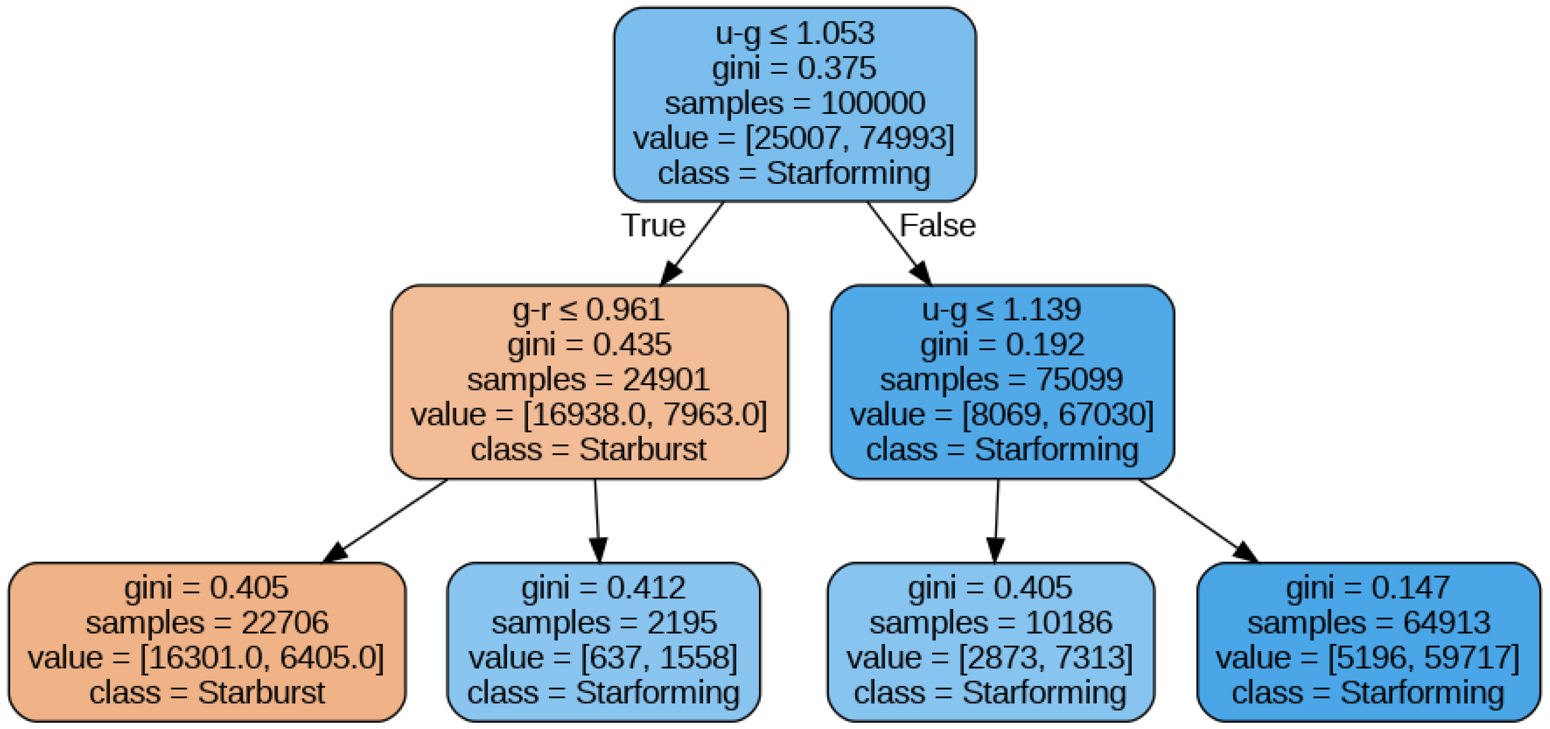
4.1.1. Gini Importance

Gini importance (GI), also known as mean decrease in impurity (MDI), assesses the importance of features in tree-based ensemble models like random forests and gradient boosted trees. Decision trees build partitions by recursively splitting nodes based on the feature and threshold that yield the greatest reduction in node impurity. The Gini importance quantifies how much the impurity decreases when a specific feature is used for splitting data at each node. Common impurity measures are the Gini impurity (for classification) or variance (for regression). The Gini impurity for a node m with K classes is calculated as

$$I_G\left(m\right)=\sum _{k=1}^K{p}_{mk}(1-p_{mk})=1-\sum _{k=1}^K{p}_{mk}^2$$

(1)

where $p_{mk}$ is the proportion of samples of class k in node m.

The importance of a feature j at a specific node m is the impurity reduction achieved by splitting on that feature at a threshold t:

$$\mathrm{\Delta }I(m,j,t)=I\left(m\right)-\left({\displaystyle \frac{N_L}{N_m}}I\left(m_L\right)+{\displaystyle \frac{N_R}{N_m}}I\left(m_R\right)\right),$$

(2)

where $N_m$, $N_L$, and $N_R$ are the number of samples in the parent and the left and right child nodes, respectively. The optimal split at the node m is determined by evaluating all available features (or a subset of them, in the case of random forests) and all possible thresholds for each of those features to maximize $\mathrm{\Delta }I$. The overall importance of feature j in a single tree T is the sum of impurity reductions at all nodes m where feature j was used for splitting, weighted by the fraction of samples reaching that node.

$$G{I}_T\left(j\right)=\sum _{m\in Nodes\left(T\right)}(N_m/N)\mathrm{\Delta }I\left(m\right).$$

(3)

For an ensemble or random forest, this is averaged over all trees.

$$G{I}_{MDI}\left(j\right)={\displaystyle \frac{1}{K}}\sum _{T=1}^{K}G{I}_T\left(j\right).$$

(4)

Features yielding larger impurity reductions across many trees are considered more important, so Gini importance can be used as a feature selection technique, where features with low Gini importance scores can be removed without significantly impacting model performance. The Gini importance is computationally efficient to compute as it is a byproduct of training. This makes it a fast and simple method for assessing feature importance. However, it is calculated on the training data which means that it can overestimate the importance of features with many possible values (high cardinality), as they have more opportunities to create splits. It may also not accurately reflect the true importance of correlated features, as it might overestimate the importance of one feature while neglecting the others. This reflects the feature’s role in the model’s internal structure rather than directly measuring its impact on predictive performance on unseen data.

4.1.2. Permutation Importance

Permutation importance (PI), also known as mean decrease in accuracy/score (MDA), is a model-agnostic technique applicable to any fitted model after training on unseen data (validation or test set). It quantifies the importance of individual input features by measuring the decrease in model performance when a feature’s values are randomly shuffled. The intuition is that if a feature is important for the model’s predictions, then scrambling its values should significantly degrade performance. The importance $I\left(j\right)$ of feature j is the difference between the baseline score and the score after permutation:

$$PI\left(j\right)=S\left(D\right)-S\left(D_j\right)$$

(5)

where S is the baseline baseline performance score (e.g., accuracy, F1-score, $R^2$, mean squared error [73]) on the validation or test dataset D, and $D_j$ is the dataset where the j-th feature column has been randomly permuted across samples. This process is often repeated multiple times with different random shuffles, and the importances are averaged for stability. A large drop $PI\left(j\right)$ indicates that the model heavily relies on feature j and that it is most important for prediction on unseen data. As this is applied on unseen data, it is considered more reliable than Gini importance and it can capture interaction effects implicitly. However, it is computationally more expensive as it requires multiple model inferences per feature and its interpretation can be complicated if input features are highly correlated, as permuting one feature may not change performance much because correlated features still contain the same information.

Feature importance measures, like Gini importance and permutation importance, are helpful in astronomical discovery and can play a role in anomaly detection. When building models to predict astronomical properties, feature importance helps to verify if the model relies on features expected to be important based on physics. For instance, if a photometric redshift model ranks specific color indices known to correlate strongly with redshift as most important, it increases confidence that the model has learned astrophysically meaningful relationships. Conversely, if a model achieves high accuracy and ranks an unexpected feature (e.g., a less commonly used color, a subtle morphological parameter) as highly important, it can prompt new scientific questions. This might suggest that this feature contains more predictive power than previously thought for that specific task or dataset, potentially leading to investigations into underlying physical reasons or revealing biases in the data. This can be a pathway to discovery by highlighting non-obvious correlations. Knowing which features are most predictive can guide astronomers in designing future surveys (e.g., prioritizing certain filters) or in refining feature extraction processes for future models. If a model performs well but relies heavily on features suspected to be related to instrumental effects or artifacts, feature importance can also flag this issue, preventing spurious scientific claims. The caveat is that feature importance primarily shows correlation and predictive power within the context of the specific model and data, not necessarily fundamental causation (Figure 1). GI and PI can be divergent; the former measures how effectively a feature is used to reduce impurity in splits in the training data, so it is reflective of the model’s construction, whereas the latter directly measures a feature’s contribution to the model’s predictive performance on unseen data. However, this information is still a valuable input for scientific reasoning and hypothesis generation. Hoyle et al. [74] found that selecting the most important photometric features and adding them to standard inputs significantly improves the accuracy and reduces catastrophic outliers in machine learning-based redshift estimations for galaxies. Gini importance has been used to show that C-class flare percentages and maximum X-ray flux are particularly critical features for solar flare forecasting [75], and permutation feature importance applied to light curve characteristics of variable stars has revealed that the importance of specific features not only depends on the classification task but also on the distance metric used [76]. Using Gini importance, [77] found that spherical overdensities, as opposed to the ellipticity and prolateness (tidal shear features), are the most important features in predicting dark matter halo masses.

4.2. Saliency-Based Methods

Deep learning models, particularly CNNs for image-based tasks and recurrent neural networks (RNNs) for sequential data, have become highly effective tools in astronomy for tasks like galaxy morphology classification, strong lens detection, or light curve analysis (e.g., [55,78,79,80]). These models, while powerful, are notoriously uninterpretable. A popular option involves generating saliency maps [81]. These methods aim to highlight which parts of the input (e.g., pixels in an image) were most influential in determining a specific output (e.g., the classification score for a particular class; see Figure 2). Techniques like integrated gradients [82] or gradient-weighted class activation mapping (Grad-CAM) [83] allow for direct comparison with known astrophysical features. In astronomy, this is especially invaluable for determining whether a model focuses on physically meaningful structures such as spiral arms, galactic bars, tidal disturbances, lensed arcs, or specific features in time series data represented as images, or are instead relying on spurious artifacts, noise patterns, or unexpected regions, potentially indicating overfitting.

In doing so, they help establish trust in the model’s predictions and reveal opportunities for scientific discovery, particularly when unexpected regions emerge as influential. They also serve a critical diagnostic function; for example, when a model produces incorrect predictions, saliency maps can expose the regions responsible, assisting in model debugging and identifying edge cases. Moreover, comparisons between models with different architectures can uncover divergent decision pathways for the same task, enriching our understanding of how model design affects interpretability.

Although often compared to attention mechanisms (Section 4.4.2), saliency methods differ in that they typically operate post hoc and offer less direct insight into internal model dynamics. They show what regions in an input affect a specific output, rather than where the model focuses on. Thus, interpreting saliency maps as full causal explanations of model behavior requires caution. Nonetheless, when integrated with astrophysical domain knowledge, saliency methods contribute not only to model validation but also to the discovery of rare or subtle phenomena that might otherwise be overlooked. Jacobs et al. [85] argue the limitation of saliency maps in a scientific context as they primarily focus on identifying important spatial regions in an input image and often lack granularity or quantitative insight into model biases and weaknesses related to other physical parameters.

4.2.1. Vanilla Saliency

The most basic saliency method computes the gradient of the model’s output score (typically the pre-activation score for the predicted class) with respect to each input pixel $x_{ij}$:

$$S_{ij}=\left|{\displaystyle \frac{\mathsf{\partial }f\left(x\right)}{\mathsf{\partial }{x}_{ij}}}\right|.$$

(6)

where $f\left(x\right)$ is the model. The magnitude of the gradient indicates sensitivity—pixels where small changes would most affect the output score are deemed important. While simple, these maps can be noisy and suffer from gradient saturation issues where the gradient can vanish or explode.

4.2.2. Guided Backpropagation or SmoothGrad

To reduce the noise present in standard gradient saliency maps, guided backpropagation [86] modifies the gradient computation by suppressing negative gradients at ReLU activation layers during the backward pass. This adjustment focuses the explanation on features that positively contribute to the model’s decision:

$${\displaystyle \frac{\mathsf{\partial }f\left(x\right)}{\mathsf{\partial }{x}_{ij}}}{|}_{guided}=\mathrm{ReLU}\left({\displaystyle \frac{\mathsf{\partial }f\left(x\right)}{\mathsf{\partial }{x}_{ij}}}\right)$$

(7)

Alternatively, SmoothGrad reduces the noise by adding noise to the input image. This results in cleaner, more focused saliency maps but can lack a clear probabilistic interpretation and and may suppress important negative evidence by design.

4.2.3. Integrated Gradients

A more theoretically robust method designed to overcome saturation issues and satisfy desirable axioms like sensitivity and completeness is integrated gradients (IGs) [82]. Instead of just using the local gradient at the input x, IG integrates the gradients along a straight-line path from a chosen baseline input $x^{\prime }$ (e.g., a black image, an average image, or an image with random noise) to the actual input x. The attribution (importance score) for the i-th input feature (pixel) $x_i$ is defined as follows:

$$I{G}_i\left(x\right)=(x^{\prime }-x){\int }_{\alpha =0}^1{\displaystyle \frac{\mathsf{\partial }f(x^{\prime }+\alpha (x-x^{\prime }))}{\mathsf{\partial }{x}_i}}d\alpha$$

(8)

In practice, this integral is typically approximated numerically. A key property is completeness: the sum of integrated gradients across all input features equals the difference between the model’s output score at the input x and the baseline $x^{\prime }$, but while providing more reliable attributions, the choice of baseline $x^{\prime }$ can significantly influence the resulting saliency map.

4.2.4. Grad-CAM (Gradient-Weighted Class Activation Mapping)

Distinct from methods that directly attribute importance to input pixels via gradients, gradient-weighted class activation mapping (Grad-CAM) [83] is specifically tailored for CNNs. It produces coarser, heatmap-style visualizations localized using the feature maps of an intermediate or deep convolutional layer (often the final one). Grad-CAM identifies image regions contributing to the prediction of a specific class c based on the activations in that layer. If $A_k$ is the k-th feature map of a chosen convolutional layer, then the weight is obtained by global average pooling the gradients,

$${\alpha }_k^c={\displaystyle \frac{1}{Z}}\sum _i\sum _j{\displaystyle \frac{\mathsf{\partial }f\left(x\right)}{\mathsf{\partial }{A}_{ij}^k}}.$$

(9)

where Z is the number of pixels in the feature map. This represents the importance of each feature map k for class c. These weights can then be used to compute a heatmap,

$$L_{Grad-CAM}^c=\mathrm{ReLU}\left(\sum _k{\alpha }_k^c{A}^k\right)$$

(10)

which highlights regions important for class c at the spatial resolution of the chosen feature map. The ReLU ensures that only features positively correlated with the class are visualized. It is typically upsampled to overlay on the original image to provide spatially coarse but semantically meaningful explanations, linking output decisions to higher-level features. Grad-CAM is especially effective in identifying higher-level structures, such as galaxy morphology or strong lensing features. However, the quality of the explanation depends on the selected convolutional layer, and different choices may lead to different interpretations. Guided GradCAM [87] combines the strengths of Grad-CAM and guided backpropagation, by performing an element-wise multiplication of their outputs. The intention is to leverage the class-discriminative localization ability of Grad-CAM as a mask for the fine-grained guided backpropagation map. This should result in a higher resolution visualization. Methods like Grad-CAM have already been widely used for interpretation of CNN models in astronomy (e.g., [57,88,89]).

While saliency methods offer intuitive visual explanations, their reliability has been increasingly questioned. Adebayo et al. [90] demonstrated that many gradient-based methods, including guided backpropagation, produce visually similar maps even when the model’s learned parameters are randomized, suggesting that these methods might be dominated by input processing such as edge detection rather than reflecting learned model knowledge. Similarly, Srinivas and Fleuret [91] argued that gradient-based explanations may primarily highlight regions causing maximal change rather than those representing meaningful semantic features used by the model. These findings highlight the importance of applying sanity checks and being cautious about over-interpreting saliency maps without rigorous validation, especially when such methods are used in scientific contexts.

4.3. Model Agnostic Methods

Model-agnostic tools like SHAP (SHapley Additive Explanations) [34] and LIME (Local Interpretable Model-Agnostic Explanations) [33] provide versatile frameworks for explaining predictions across a wide range of model types. SHAP values offer a theoretically grounded decomposition of predictions into feature contributions, while LIME fits simple surrogate models in the local neighborhood of a prediction to approximate the behavior of the full model. Both are widely used to evaluate feature relevance, detect biases, and facilitate model debugging, though they come with limitations.

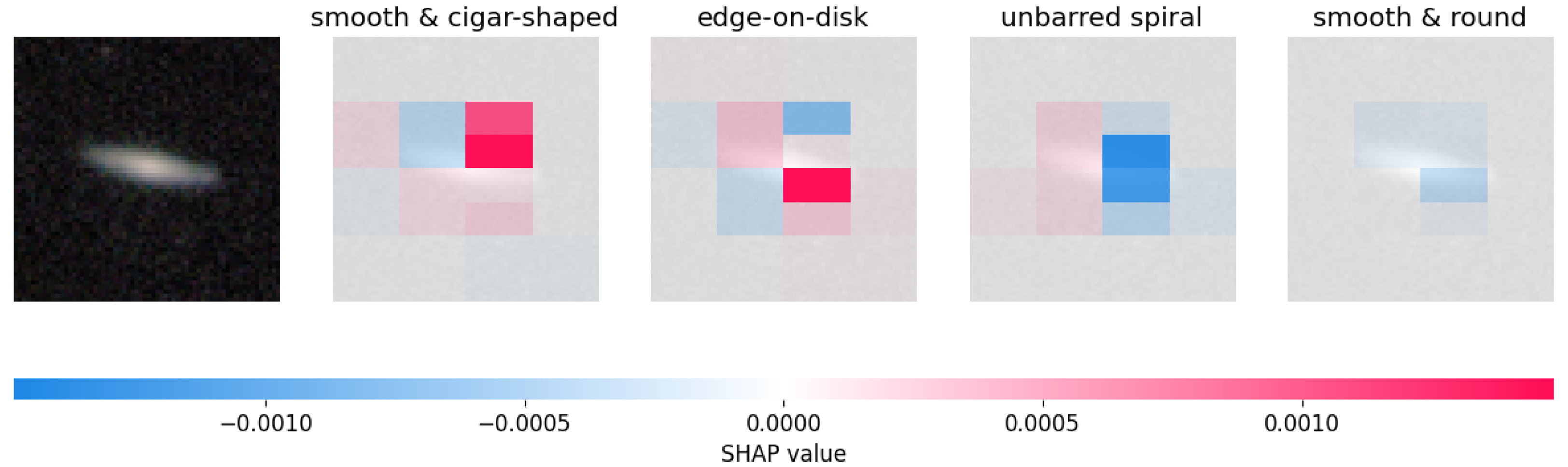
4.3.1. SHAP: SHapley Additive Explanations

SHAP values (Figure 3) are based on the concept of Shapley values from cooperative game theory [92]. Given a function f representing the model’s prediction, the goal is to assign a value ${\varphi }_i$ to each feature $x_i$ such that

$$f\left(x\right)={\varphi }_0+\sum _{i=1}^n{\varphi }_i,$$

(11)

where ${\varphi }_0$ is the expectation value (i.e., the baseline prediction when no features are present), and each ${\varphi }_i$ represents the contribution of feature i to the prediction for input x.

Formally, the Shapley value for feature i is defined as

$${\varphi }_i=\sum _{S\subseteq N\left\{i\right\}}{\displaystyle \frac{\left|S\right|!\left(\right|N|-|S|-1)!}{\left|N\right|!}}(f_x(S\cup \left\{i\right\})-f_x\left(S\right))$$

(12)

where N is the set of all the features, and $f_x\left(S\right)=E\left[f\left(X\right)\right|X_S=x_S]$ is the expected output of the model conditional on knowing the values $x_S$ for features in subset S. This expectation is often approximated using a background dataset or other techniques. $f_x(S\cup \left\{i\right\})$ is similarly defined when feature i is also known. The term $[f_x(S\cup \left\{i\right\})-f_x\left(S\right)]$ represents the marginal contribution of adding feature i to the subset S. The combinatorial term weights this contribution according to its position in all possible feature orderings. While SHAP is primarily designed for local interpretability (explaining individual predictions), it can also produce global explanations by aggregating local explanations across multiple instances, visualizing them through SHAP summary and dependence plots.

SHAP values provide feature attributions satisfying several desirable properties that contribute to their theoretical appeal. These include efficiency (the sum of feature contributions equals the difference between the prediction and the baseline), symmetry (features contributing identically receive the same attribution), the dummy property (features having no effect on the prediction receive zero attribution), and additivity (the SHAP values for combined models are the sum of the values from individual models). However, computing exact Shapley values is typically computationally intractable for models with many features. Consequently, practical SHAP implementations rely on efficient approximations or model-specific algorithms, such as the popular TreeSHAP for tree-based ensembles, to estimate these values efficiently. SHAP has been used to understand molecular abundances in star-forming regions. Heyl et al. [93] were able to quantify parameters on molecular abundances; for example, they discovered that H₂O and CO’s gas phase abundances depend strongly on the metallicity, as well as reconfirming other known relationships with abundances, and Ye et al. [94] used SHAP to identify five key absorption features in spectra for carbon star identification.

4.3.2. LIME: Local Interpretable Model-Agnostic Explanations

LIME (Figure 4) takes a different approach operating on a simple, intuitive principle to approximate the behavior of a complex, potentially non-linear model f in the local neighborhood of a specific input instance x using a simpler, inherently interpretable surrogate model g (e.g., a sparse linear model or a shallow decision tree). For a linear model, the explanation g for an instance $z^{\prime }$ (a simplified, interpretable representation of z) takes the form

$$g\left(z^{\prime }\right)=w_g{z}^{\prime },$$

(13)

where $w_g$ are the weights (feature importances) to be learned. LIME constructs a local dataset by perturbing the original input and observing the model’s response:

$$\mathcal{L}(f,g,{\pi }_x)=\sum _{z\in Z}{\pi }_x\left(z\right){(f\left(z\right)-g\left(z^{\prime }\right))}^2+{\mathrm{\Omega }}_g$$

(14)

This loss function measures how well g approximates f for the perturbed samples z weighted by their proximity ${\pi }_x$, which defines the neighborhood around x. To ensure that the explanation g remains interpretable, a complexity penalty ${\mathrm{\Omega }}_g$ is added. For linear models, this might encourage sparsity (e.g., minimizing the number of non-zero weights or using an L1-norm penalty). For decision trees, it might penalize depth. The surrogate model g is trained to minimize $\mathcal{L}$, yielding feature weights that approximate the influence of each input feature locally. Unlike SHAP, LIME does not require exhaustive enumeration of feature subsets and is computationally more efficient, but its explanations can vary depending on the sampling process and surrogate complexity. In classifying galaxy morphologies, Goh et al. [95] showed that LIME enabled the effective identification of influential regions in the image but also showed that the model utilized some unexpected image regions beyond the galaxy object itself for classification, potentially an area of bias inherent in the images.

4.4. Interpretable Models by Design

While post hoc explanations for “black-box” models, particularly deep neural networks, are widely used ultimately, they are based on approximations that can be misleading. An alternative and growing field focuses on designing model architectures that are inherently structured for transparency, facilitating direct interpretation (e.g., linear regression, decision trees). In these models, the explanations are the model itself, offering stronger foundations for trust, transparency, and fairness that is especially critical in areas where the decision stakes are high. However, it is important to remember the trade-off between interpretability and accuracy, especially in high-dimensional, non-linear tasks. Inherently interpretable models are typically more limited (e.g., simpler models), and performance accuracy is often lower on complex tasks. We now explore some of these approaches in more detail.

4.4.1. Rule-Based Methods

Feature importance techniques (like Gini or permutation importance) tell us which features the model found most influential in general. Rule-based approaches represent a class of inherently interpretable models that aim for complete transparency in their decision-making process through their structure. The most common example is the decision tree [96], where predictions are made by following a specific path of IF–THEN conditions from a root node to a leaf node, based on thresholds applied to input feature values (Figure 5).

This explicit logic chain makes it straightforward, in principle, to understand exactly how a specific prediction was derived for any given input instance. Other methods, like rule lists or algorithms such as RuleFit [97], explicitly generate sets of rules often combined with linear models.

The primary strength of these methods lies in their high interpretability and transparency. The decision logic is human-readable, making them intuitive and particularly useful in classification tasks requiring well-defined decision boundaries or where explaining the reasoning to stakeholders is paramount. They can also naturally capture interaction effects between features within a single rule path. But, despite their transparency, rule-based methods often have limited flexibility and expressive power, particularly when dealing with the complex, high-dimensional, and often noisy data typical of modern astronomical surveys where intricate non-linear relationships may exist. Very deep decision trees, while technically transparent, can become visually complex and difficult for humans to fully grasp. Furthermore, tree structures can be unstable. Small variations in the training data can lead to significantly different trees and rules. Consequently, they may achieve lower predictive accuracy compared to ensemble methods or deep learning models on many complex astronomical tasks.

While perhaps less frequently deployed for achieving state-of-the-art performance on complex raw data analysis today, rule-based logic remains conceptually valuable. Simple decision trees have been used for basic classification tasks (e.g., star/galaxy separation based on magnitude and morphology metrics (e.g., [98])) or formed components of early transient alert systems [99]. More complex rule-based classification algorithms like random forests can effectively learn the complex relationship between the initial density field conditions of dark matter particles and their final state (whether they end up in massive halos), allowing for accurate prediction of simulation outcomes without running the full simulation [100].

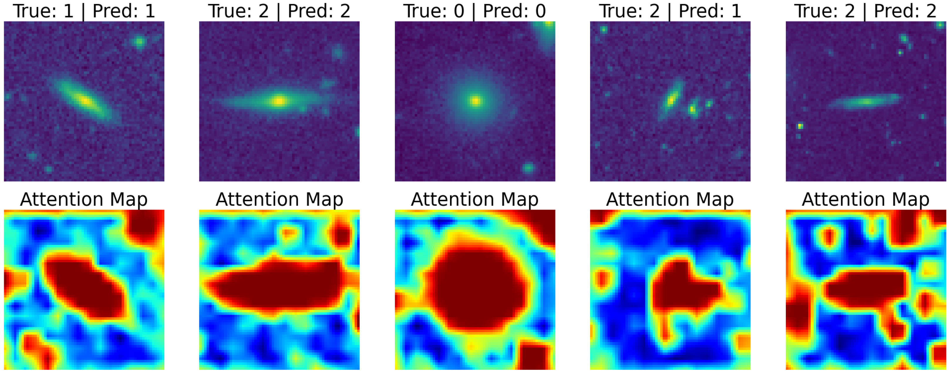
4.4.2. Attention Mechanisms

Often compared to saliency are attention mechanisms. Initially developed to improve performance in tasks like machine translation [101], they have been increasingly integrated into neural architectures [35]. They offer a natural interface for interpretability beyond simply analyzing feature rankings or explicit rules by highlighting which parts of the input (e.g., image regions, sequence elements, specific features) the model focuses on when generating an output.

The core idea behind attention is to allow a model to dynamically weigh the importance of different parts of its input data, rather than relying solely on fixed-size receptive fields (as is standard in CNNs) or compressing all prior information into a single hidden state vector (as in basic RNNs). When processing an element (e.g., predicting the next word in a sentence, classifying an image), the attention mechanism computes a set of weights called attention scores over the input elements, indicating how much attention or importance should be given to each one.

A dominant form of attention, particularly central to the influential Transformer architecture [35], is scaled dot-product attention, also known as self-attention (Figure 6). Mathematically, the self-attention mechanism computes attention scores as follows:

$$\alpha =softmax\left({\displaystyle \frac{Q·K}{\sqrt{d}}}\right)$$

(15)

With the final weighted output representation:

$$Attention(Q,K,V)=\alpha V$$

(16)

where the queries (Q), keys (K), and values (V) are vectors derived from the input embeddings. Query (Q) represents the current element or context asking for information (“What am I looking for?”). Key (K) represents identifiers or labels for the input elements (“What information does this element have?”), and value (V) represents the actual content or features of the input elements associated with the keys. The dimensionality of the key vectors d is used for scaling, and the resulting attention matrix $\alpha$ is often treated as a measure of interpretability. It can be visualized to inform use about which input tokens or spatial regions in an image the model focused on.

Self-attention computes the relevance of different parts of the input sequence to each other. But a single attention layer might only capture one type of relationship (e.g., similarity in spatial location or color in an image, or proximity in time in a light curve). To address this, multi-head attention runs several attention mechanisms in parallel (“heads”), each with its own learnable parameters, allowing the model to jointly attend to information from different representation subspaces at different positions. The outputs from all heads are concatenated and projected.

Attention mechanisms are inherently more interpretable than traditional deep learning layers, because they produce explicit, learnable weights that can be visualized and analyzed (Figure 7). These attention scores can be mapped back to domain-specific structures: pixels in an image, time points in a signal, or wavelengths in a spectrum—offering intuitive insights for scientists. Like feature importance, attention is not an anomaly detector, per se, but when a model flags a galaxy or transient as unusual, the attention map can reveal which regions of the image or spectral range triggered the anomaly, and whether the model is focusing on meaningful astrophysical structure or noise/artifacts. This grounds the anomaly score in interpretable terms. Attention maps can also help filter false positives by revealing when the model’s focus is on irrelevant regions (e.g., image borders, artifacts). However, a significant body of research argues that attention weights are not a direct or reliable explanation of model predictions [102]. Reasons include that high attention does not guarantee causality, the complex non-linear transformations after the attention layer can influence the final prediction, and the attention weights can sometimes be manipulated without significantly changing the model’s output, whilst equally significant are challenges against those claims [103]. In any case, while attention maps offer valuable insight into the model’s internal processing and where it looks, they should be interpreted with caution. They are a potentially useful diagnostic tool but not necessarily a faithful explanation of why a prediction was made. Ref. [104] used attention-gating not only to improve their classification of radio galaxies but also to help choose models that align better with how astronomers classify radio sources by eye.

4.4.3. Symbolic Regression

Symbolic regression is an interpretable machine learning technique that seeks to discover analytical expressions that best model a given dataset, without assuming a predefined functional form (like linear regression or neural networks). Unlike traditional regression methods that fit coefficients to a fixed equation, symbolic regression algorithms explore a combinatorial space of mathematical operators (e.g., +, −, ×, ÷, exp, log) and input features to construct candidate models [105]. The objective is to minimize a loss function $\mathcal{L}(y,\widehat{y})$ while simultaneously optimizing for simplicity and parsimony, often guided by multi-objective optimization:

$$\underset{f\in F}{min}(\mathcal{L}(y,f\left(x\right))+\lambda Complexity\left(f\right)),$$

(17)

where F denotes the space of symbolic expressions, and $Complexity\left(f\right)$ is a regularization term penalizing complexity.

The primary appeal of SR lies in its potential for high interpretability and transparency. The direct output is a human-readable mathematical formula, representing perhaps the ultimate form of a “white-box” model. If the discovered equation is compact, accurate, and physically plausible, it can provide profound scientific insight, potentially revealing previously unknown empirical relationships or even approximations to fundamental physical laws directly from data [106,107]. This contrasts sharply with black-box models where the learned relationships are opaque. This approach is particularly compelling in physics-informed contexts, where the recovery of closed-form expressions aligns with scientific intuition and the formulation of empirical or theoretical laws. SR can generate simple, interpretable analytical approximations for complex physical simulations or theoretical functions where a readily understandable formula is desired [108] and in astronomy, symbolic regression has been used to rediscover known physical laws from simulated data and holds promise for uncovering novel empirical scaling relations between galaxy properties, parameters describing stellar evolution, or equations governing orbital dynamics directly from observational or simulation data [109,110,111].

Despite its interpretability, SR faces several limitations. The search space is typically vast and non-convex, often requiring evolutionary algorithms (e.g., genetic programming) or more recent neural-guided approaches (e.g., deep symbolic regression) to navigate efficiently. As a result, symbolic regression can be computationally expensive, especially in high-dimensional settings where many candidate expressions must be evaluated. Additionally, symbolic models may be sensitive to noise, and the lack of strong priors can lead to overfitting or implausible expressions in data-poor regimes.

Nevertheless, SR offers a rare combination of accuracy and explicitness that makes it a valuable tool for hypothesis generation and scientific insight in astronomy. Its outputs are interpretable, closed-form equations that can be scrutinized, validated, or rejected in the light of physical principles, fostering a deeper understanding of the patterns uncovered by machine learning. Wadekar et al. [112] trained a neural network to predict neutral hydrogen content from dark matter fields. The saliency maps revealed that the neural network considered the halo’s environment, not just the halo itself, when making predictions, motivating the closer exploration of assembly bias. Using SR, they were able to parameterize a new and physically interpretable model of assembly bias.

4.4.4. Learning Interpretable Latent Representations

In some machine learning models, particularly those involving dimensionality reduction like autoencoders, the input data are transformed into a latent space. This space is a lower-dimensional, abstract representation where the original data are encoded, often in a compressed form. While this encoding is structured, it is not automatically understandable by humans unless the model is specifically designed to be so. Interpretability in latent spaces means understanding what each latent variable encodes, with, ideally, each dimension corresponding to a distinct, meaningful factor of variation (e.g., one variable controls rotation, another controls scale). This can be encouraged through the following:

• Disentanglement techniques, which aim to separate independent factors of variation in the latent representation by adding additional constraints to the loss function to encourage each latent dimension to capture an independent aspect of the data. Models like $\beta$-variational autoencoders ($\beta$-VAEs) or other disentangled VAEs perform this. The $\beta$-VAE loss is defined as

  $$L=L_{reconstruction}+\beta D_{KL}(q_{\varphi }\left(z\right|x)\left|\right|p\left(z\right))$$

  (18)

  where $L_{reconstruction}$ is the original loss, $D_{KL}(q_{\varphi }\left(z\right|x)\left|\right|p\left(z\right))$ is the Kullback–Leibler (KL) divergence that measures how much the learned latent distribution $q_{\varphi }\left(z\right|x)$ deviates from a chosen prior distribution $p\left(z\right)$ (typically a standard Gaussian), and the hyperparameter $\beta$ encourages the model to learn a latent distribution that is closer to the simple prior and, thus, promotes disentanglement.
• Conditional generation models like conditional variational autoencoders (CVAEs) condition the model on known variables like class labels. By observing how the latent space changes when conditioned on different known variables, its possible to infer how certain learned features in the latent space relate to these explicit conditions.
• Latent traversals involve systematically changing one latent variable at a time (while keeping others fixed) and observing the generated outputs. This technique can reveal what each dimension represents and whether it aligns with human-understandable concepts.
• Post hoc analysis of latent space structure: After training, dimensionality reduction techniques like principal component analysis (PCA) and clustering on the latent space can be an effective way to further explore the latent space to gain insights to what the model has learned.

An application of these principles is demonstrated by [113] who trained a variational encoder using a $\beta$-VAE loss to predict the halo mass function (HMF) by compressing it into a three-dimensional latent space. Post training, they use mutual information analysis to understand the cosmological dependence of each latent variable. Notably, one latent variable captured non-universal HMF behavior, linking it to the Universe’s recent growth history after matter–dark-energy equality, suggesting that subtle differences in the Universe’s expansion history after dark energy becomes dominant, leading to the deviations from universality.

However, learning latent variables that align with human-understandable concepts remains challenging [114]. Even disentangled latent variables might not consistently map semantic features, and for models like VAEs, the latent space is probabilistic (variables are samples from distributions). This inherent randomness can add a layer of complexity when trying to interpret the precise meaning of the encoding for individual data points.

4.4.5. Physics-Informed Neural Networks (PINNs)

Whilst not intrinsically interpretable in the same way that simpler models like linear regression or decision trees are, physics-informed neural networks (PINNs) possess characteristics that make them more interpretable than standard “black-box” neural networks. These networks incorporate knowledge of physical laws, often as partial differential equations (PDEs), into the loss function used to train the neural network [115]. This architectural bias ensures that the model predictions remain consistent with established physical principles. We can interpret their outputs in the context of these laws, and we can trust that the model’s behavior is, to some extent, governed by these principles, enhancing their transparency and trustworthiness. By encoding domain knowledge directly into the model structure, PINNs help bridge the gap between black-box neural networks and physically interpretable modeling; however, despite their promise, challenges remain in training efficiency, handling stiff PDEs, and scaling to high dimensions [116].

4.5. Prototypes and Exemplars

While many interpretability methods are benchmarked on supervised tasks due to the presence of a ground truth, understanding the outputs of unsupervised methods like clustering is also needed. Here, interpretability often shifts to understanding the defining characteristics of the discovered groups or structures and assessing their astrophysical relevance, rather than explaining a singular prediction. This can be challenging as there is no ground truth and, hence, no explanation target, and quantitative evaluation of interpretation correctness is less straightforward. An intuitive approach is then reasoning by analogy, explaining predictions by comparing new inputs to known examples from the training set. These prototype- and exemplar-based methods offer explanations by referencing representative data points from the training set, grounding a model’s decision to specific instances rather than abstract features or internal model mechanics [117]. They operate on the principle “This input is class Y because it resembles these known examples of Y”, requiring a meaningful similarity function defined either in the original feature space or a learned embedding space.

Two main variants exist. Exemplar-based methods, like k-nearest neighbors, use actual training data points, making predictions directly traceable to real observations. Prototype-based methods instead use learned or synthetic representatives (e.g., cluster centroids or learned latent prototypes) that act as archetypes for a class, summarizing groups of examples. Unsupervised learning techniques [70] are frequently used to discover or define potential prototypes or to create the feature space in which exemplars are identified. The appeal lies in their alignment with human reasoning, mirroring how astronomers interpret visual data (e.g., classifying galaxies by comparison, as in Galaxy Zoo) or time series data (e.g., comparing supernova light curves). This approach is also useful for model debugging, allowing inspection of influential examples to diagnose issues like overfitting or dataset biases.

However, limitations exist. Effectiveness hinges on the quality and interpretability of the chosen similarity metric, as proximity in high-dimensional or latent spaces may not reflect true semantic similarity. These methods typically provide only local explanations, can be computationally demanding for large datasets, and often lack feature level granularity, explaining that an input is similar but not which features drive the similarity.

Despite these challenges, prototype- and exemplar-based explanations remain valuable, particularly when intuitive, traceable interpretations grounded in real data are needed. In astronomy, where expert visual inspection is common, they help bridge the gap between complex model outputs and scientific understanding.

4.6. AI Reasoning Models

One area that is seeing significant benefits of xAI is, surprisingly, large language models (LLMs). Traditional LLMs excel at generating text and answering questions, but they often struggle with tasks requiring logical deduction or multi-step problem solving. Their adoption in scientific research is, therefore, often hindered by limitations such as a tendency for generating plausible but incorrect results and a lack of true understanding of underlying principles. The lack of transparency in how these models arrive at their conclusions makes it difficult to validate their results and build trust in their predictions, especially when applied in astronomy where verifiable logic is paramount. As LLMs become integrated into scientific workflows, from data analysis to hypothesis generation, we need to ensure that we understand how they arrive at their outputs. Methods like chain-of-thought (CoT) and question–analysis prompting guide models to reason step-by-step, improving performance on complex tasks and offering a degree of process transparency [118,119]. These techniques allow users to follow and evaluate the logic behind model outputs, helping to catch errors and build trust.

However, this surface-level reasoning can mask deeper issues. CoT outputs may appear logical but do not necessarily reflect the model’s true internal processes [120,121,122]. Caution is warranted, as CoT’s seemingly logical steps may not be faithful [123], potentially representing post hoc rationalizations, flawed logic, or pattern mimicry instead of true reasoning. Faithfulness remains difficult to measure, existing metrics are debated [124], and CoT reasoning is vulnerable to adversarial attacks [125]. This highlights a broader challenge: enhancing interpretability in AI-driven science not just through better outputs, but through better understanding of model behavior. The emergence of agentic systems like the AI Scientist-v2 [126] and AI Cosmologist [127] are moving us towards fully automated research pipelines, from hypothesis generation to code implementation and analysis, further emphasizing the rapid developments in AI and the need for transparent and trustworthy reasoning for a future in astronomy that uses AI responsibly.

5. Navigating the Future and Concluding Remarks

Artificial intelligence is rapidly advancing astronomical discovery; yet, moving forward, the successful integration of it into the core of astronomical research requires more than just predictive accuracy. The ultimate scientific value of these powerful tools hinges critically on our ability to understand, validate, and trust their outputs through interpretable and explainable methodologies.

Despite progress, the practical application of trustworthy and interpretable AI in astronomy faces substantial open challenges and limitations. A primary concern is scalability; many sophisticated xAI techniques (such as model-agnostic methods like LIME and SHAP that require multiple model evaluations, or symbolic regression with its vast search space for expressions) incur significant computational costs, making their application to the petabyte- and exabyte-scale datasets from facilities like LSST or SKA, or to increasingly complex deep learning models, a major bottleneck [128], hindering their effective use in real-time transient astronomy. Fundamental questions also persist about the faithfulness of explanation and the reliability of the training data, including whether data uncertainties are adequately considered. For instance, while visually appealing, vanilla saliency maps can be noisy and sensitive to model architecture. GradCAM can be too coarse, leading to missed fine-grained features. Likewise, attention mechanisms, despite being inherent to the model, can be misleading, potentially highlighting correlations rather than causal links. Furthermore, some saliency methods have been shown to be insensitive to model parameter and label randomization, questioning their dependency on learned parameters [37,90,129]. This issue extends to other methods: LIME explanations are highly sensitive to perturbation strategy and kernel width, and its linear approximations may capture non-linear behaviors; permutation-based feature importance can be misleading for highly correlated features; and achieving true, meaningful disentanglement in latent spaces of interpretable-by-design models like $\beta$-VAEs remains notoriously difficult. Compounding this is the lack of standardized benchmarks and evaluation metrics specifically tailored for assessing explanation quality within the astronomical context [130,131]. Even when explanations are generated, their potential complexity can make them difficult for domain scientists to interpret effectively, hindering actionable insights. Given these varied limitations, it is clear that no single xAI method offers a complete understanding. Relying on just one technique risks painting a biased picture. We, therefore, encourage the reader to employ and compare a range of interpretability methods and look for consensus. If different methods highlight similar features or patterns, confidence in the interpretation increases. It is also imperative to test explanations, for example, by observing how the model’s prediction changes when that feature is perturbed or removed. Furthermore, as different training runs can produce equally valid but non-unique networks, the robustness of explanations to such variations must be considered. Addressing this full spectrum of challenges necessitates developing more efficient, demonstrably faithful xAI methods, alongside tools and interfaces that lower the barrier for user expertise.

Beyond these technical hurdles lie important ethical considerations. While large public astronomical datasets generally pose minimal individual privacy risks compared to other fields [132], responsible data governance, including equitable access to data and tools, and transparency in methodology remain crucial. A significant ethical challenge is mitigating bias; AI models trained on historical astronomical data can inadvertently learn and perpetuate observational selection effects or existing societal biases present in data collection or labeling, potentially leading to skewed scientific conclusions. Interpretable AI methods are vital tools for detecting and potentially mitigating these biases, ensuring fairness and robustness in scientific findings. Responsible use also demands transparency from researchers regarding their use of AI and xAI methods, including acknowledging limitations. Over-reliance on complex models without adequate interpretation, or using explanations to simply reinforce preexisting beliefs, could undermine the scientific process itself. Addressing this full spectrum of technical, practical, and ethical challenges through continued research and interdisciplinary dialogue is essential for the responsible and effective advancement of AI-driven discovery in astronomy.

Despite the challenges, the future of interpretable machine learning in astronomy discovery looks promising. Significant advancements are being pursued in deep learning interpretability, moving beyond surface-level explanations towards mechanistic interpretability aiming to reverse engineer the specific algorithms learned within complex neural networks [133]. There is also exciting potential in leveraging ML for causal inference, enabling a shift from identifying correlations to understanding cause-and-effect relationships directly from astronomical data [134]. Furthermore, the synergy between physics-informed machine learning [135,136], which embeds physical laws into models, and xAI techniques promises models that are not only potentially more robust but also interpretable by design. Future directions also include developing hybrid AI systems (e.g., neural-symbolic) and domain-specific interpretability methods tailored to the unique characteristics of astronomical data (images, spectra, time series, simulations), alongside more robust techniques for evaluating the faithfulness and utility of explanations [137]. These trends collectively point towards a future where AI serves as a more transparent, reliable, and insightful partner in astronomical discovery.

Advancing trustworthy AI in astronomy fundamentally requires closer interdisciplinary collaboration and the establishment of shared best practices. Fostering joint workshops, dedicated funding initiatives supporting cross-domain teams, and developing common software libraries tailored for astronomical data can bridge the gap between AI researchers and domain scientists. Simultaneously, the community should work towards standardizing IML workflows: developing guidelines for the application and reporting of explainability methods in publications, creating astronomy-specific benchmarks to objectively evaluate different techniques, and promoting open-source sharing of models and interpretation code. Such concerted efforts will accelerate the development and responsible adoption of robust, reliable, and truly insightful interpretable machine learning tools for astronomical discovery.

This review surveyed the profound impact of artificial intelligence on astronomical discovery, demonstrating its necessity in the face of exponentially growing data. The central takeaway, however, is that predictive power alone is insufficient for scientific progress; it must be built upon a foundation of trust, which is cultivated through interpretability and explainability. Understanding how and why AI models arrive at their conclusions allows astronomers to validate findings, debug complex systems, guard against bias, and discover new scientific insights directly from the learned representations. We collated some key interpretation tools, but addressing the current limitations in xAI and embracing emerging trends towards more transparent, causal, and physically grounded models is a still an ongoing endeavor for the future of the field. Ultimately, through the adoption of best practices by prioritizing interpretability alongside predictive performance, trustworthy AI will become an indispensable and reliable partner for astronomical discovery.

References

1. Hubble, E.P. A spiral nebula as a stellar system, Messier 31. Astrophys. J. 1929, 69, 103–158. [Google Scholar] [CrossRef]
2. Benn, C.R.; Sanchez, S.F. Scientific impact of large telescopes. Publ. Astron. Soc. Pac. 2001, 113, 385. [Google Scholar] [CrossRef]
3. O’Riordan, C.; Oldham, L.; Nersesian, A.; Li, T.; Collett, T.; Sluse, D.; Altieri, B.; Clément, B.; Vasan, K.; Rhoades, S.; et al. Euclid: A complete Einstein ring in NGC 6505. Astron. Astrophys. 2025, 694, A145. [Google Scholar] [CrossRef]
4. Martinez-Delgado, D.; Stein, M.; Pawlowski, M.S.; Makarov, D.; Makarova, L.; Donatiello, G.; Lang, D. Tracing satellite planes in the Sculptor group: II. Discovery of five faint dwarf galaxies in the DESI Legacy Survey. arXiv 2024, arXiv:2405.03769. [Google Scholar]
5. MacDonald, E.A.; Donovan, E.; Nishimura, Y.; Case, N.A.; Gillies, D.M.; Gallardo-Lacourt, B.; Archer, W.E.; Spanswick, E.L.; Bourassa, N.; Connors, M.; et al. New science in plain sight: Citizen scientists lead to the discovery of optical structure in the upper atmosphere. Sci. Adv. 2018, 4, eaaq0030. [Google Scholar] [CrossRef]
6. Lintott, C.J.; Schawinski, K.; Slosar, A.; Land, K.; Bamford, S.; Thomas, D.; Raddick, M.J.; Nichol, R.C.; Szalay, A.; Andreescu, D.; et al. Galaxy Zoo: Morphologies derived from visual inspection of galaxies from the Sloan Digital Sky Survey. Mon. Not. R. Astron. Soc. 2008, 389, 1179–1189. [Google Scholar] [CrossRef]
7. York, D.G.; Adelman, J.; Anderson Jr, J.E.; Anderson, S.F.; Annis, J.; Bahcall, N.A.; Bakken, J.; Barkhouser, R.; Bastian, S.; Berman, E.; et al. The sloan digital sky survey: Technical summary. Astron. J. 2000, 120, 1579. [Google Scholar] [CrossRef]
8. Kaiser, N.; Aussel, H.; Burke, B.E.; Boesgaard, H.; Chambers, K.; Chun, M.R.; Heasley, J.N.; Hodapp, K.W.; Hunt, B.; Jedicke, R.; et al. Pan-STARRS: A large synoptic survey telescope array. In Proceedings of the Survey and Other Telescope Technologies and Discoveries; SPIE: Bellingham, WA, USA, 2002; Volume 4836, pp. 154–164. [Google Scholar]
9. Ivezić, Ž.; Kahn, S.M.; Tyson, J.A.; Abel, B.; Acosta, E.; Allsman, R.; Alonso, D.; AlSayyad, Y.; Anderson, S.F.; Andrew, J.; et al. LSST: From science drivers to reference design and anticipated data products. Astrophys. J. 2019, 873, 111. [Google Scholar] [CrossRef]
10. Dewdney, P.E.; Hall, P.J.; Schilizzi, R.T.; Lazio, T.J.L. The square kilometre array. Proc. IEEE 2009, 97, 1482–1496. [Google Scholar] [CrossRef]
11. Laureijs, R.; Amiaux, J.; Arduini, S.; Augueres, J.L.; Brinchmann, J.; Cole, R.; Cropper, M.; Dabin, C.; Duvet, L.; Ealet, A.; et al. Euclid definition study report. arXiv 2011, arXiv:1110.3193. [Google Scholar]
12. Gardner, J.P.; Mather, J.C.; Clampin, M.; Doyon, R.; Greenhouse, M.A.; Hammel, H.B.; Hutchings, J.B.; Jakobsen, P.; Lilly, S.J.; Long, K.S.; et al. The james webb space telescope. Space Sci. Rev. 2006, 123, 485–606. [Google Scholar] [CrossRef]
13. Spergel, D.; Gehrels, N.; Baltay, C.; Bennett, D.; Breckinridge, J.; Donahue, M.; Dressler, A.; Gaudi, B.; Greene, T.; Guyon, O.; et al. Wide-field infrarred survey telescope-astrophysics focused telescope assets WFIRST-AFTA 2015 report. arXiv 2015, arXiv:1503.03757. [Google Scholar]
14. Vogelsberger, M.; Marinacci, F.; Torrey, P.; Puchwein, E. Cosmological simulations of galaxy formation. Nat. Rev. Phys. 2020, 2, 42–66. [Google Scholar] [CrossRef]
15. Skoda, P.; Adam, F. Knowledge Discovery in Big Data from Astronomy and Earth Observation: AstroGeoInformatics; Elsevier: Amsterdam, The Netherlands, 2020. [Google Scholar]
16. Collaboration, E.; Böhringer, H.; Chon, G.; Cucciati, O.; Dannerbauer, H.; Bolzonella, M.; De Lucia, G.; Cappi, A.; Moscardini, L.; Giocoli, C.; et al. Euclid preparation. Astron. Astrophys. 2025, 693, A58. [Google Scholar] [CrossRef]
17. Narayan, G.; Zaidi, T.; Soraisam, M.D.; Wang, Z.; Lochner, M.; Matheson, T.; Saha, A.; Yang, S.; Zhao, Z.; Kececioglu, J.; et al. Machine-learning-based Brokers for Real-time Classification of the LSST Alert Stream. Astrophys. J. Suppl. Ser. 2018, 236, 9. [Google Scholar] [CrossRef]
18. Lieu, M.; Cheng, T.Y. Machine Learning methods in Astronomy. Astron. Comput. 2024, 47, 100830. [Google Scholar] [CrossRef]
19. Mehta, P.; Bukov, M.; Wang, C.H.; Day, A.G.; Richardson, C.; Fisher, C.K.; Schwab, D.J. A high-bias, low-variance introduction to machine learning for physicists. Phys. Rep. 2019, 810, 1–124. [Google Scholar] [CrossRef]
20. Graham, M.J.; Kulkarni, S.; Bellm, E.C.; Adams, S.M.; Barbarino, C.; Blagorodnova, N.; Bodewits, D.; Bolin, B.; Brady, P.R.; Cenko, S.B.; et al. The zwicky transient facility: Science objectives. Publ. Astron. Soc. Pac. 2019, 131, 078001. [Google Scholar] [CrossRef]
21. Masci, F.J.; Laher, R.R.; Rusholme, B.; Shupe, D.L.; Groom, S.; Surace, J.; Jackson, E.; Monkewitz, S.; Beck, R.; Flynn, D.; et al. The zwicky transient facility: Data processing, products, and archive. Publ. Astron. Soc. Pac. 2018, 131, 018003. [Google Scholar] [CrossRef]
22. Mahabal, A.; Rebbapragada, U.; Walters, R.; Masci, F.J.; Blagorodnova, N.; van Roestel, J.; Ye, Q.Z.; Biswas, R.; Burdge, K.; Chang, C.K.; et al. Machine learning for the zwicky transient facility. Publ. Astron. Soc. Pac. 2019, 131, 038002. [Google Scholar] [CrossRef]
23. Metzger, B.D.; Berger, E. What is the most promising electromagnetic counterpart of a neutron star binary merger? Astrophys. J. 2012, 746, 48. [Google Scholar] [CrossRef]
24. Jia, P.; Jia, Q.; Jiang, T.; Yang, Z. A simulation framework for telescope array and its application in distributed reinforcement learning-based scheduling of telescope arrays. Astron. Comput. 2023, 44, 100732. [Google Scholar] [CrossRef]
25. Adadi, A.; Berrada, M. Peeking inside the black-box: A survey on explainable artificial intelligence (XAI). IEEE Access 2018, 6, 52138–52160. [Google Scholar] [CrossRef]
26. Kamath, U.; Liu, J. Explainable Artificial Intelligence: An Introduction to Interpretable Machine Learning; Springer Nature: Berlin/Heidelberg, Germany, 2021. [Google Scholar]
27. Ćiprijanović, A.; Kafkes, D.; Snyder, G.; Sánchez, F.J.; Perdue, G.N.; Pedro, K.; Nord, B.; Madireddy, S.; Wild, S.M. DeepAdversaries: Examining the robustness of deep learning models for galaxy morphology classification. Mach. Learn. Sci. Technol. 2022, 3, 035007. [Google Scholar] [CrossRef]
28. Walmsley, J. Artificial intelligence and the value of transparency. AI Soc. 2021, 36, 585–595. [Google Scholar] [CrossRef]
29. Montavon, G.; Samek, W.; Müller, K.R. Methods for interpreting and understanding deep neural networks. Digit. Signal Process. 2018, 73, 1–15. [Google Scholar] [CrossRef]
30. Zhang, Y.; Tiňo, P.; Leonardis, A.; Tang, K. A survey on neural network interpretability. IEEE Trans. Emerg. Top. Comput. Intell. 2021, 5, 726–742. [Google Scholar] [CrossRef]
31. Gunning, D.; Stefik, M.; Choi, J.; Miller, T.; Stumpf, S.; Yang, G.Z. XAI—Explainable artificial intelligence. Sci. Robot. 2019, 4, eaay7120. [Google Scholar] [CrossRef]
32. Arrieta, A.B.; Díaz-Rodríguez, N.; Del Ser, J.; Bennetot, A.; Tabik, S.; Barbado, A.; García, S.; Gil-López, S.; Molina, D.; Benjamins, R.; et al. Explainable Artificial Intelligence (XAI): Concepts, taxonomies, opportunities and challenges toward responsible AI. Inf. Fusion 2020, 58, 82–115. [Google Scholar] [CrossRef]
33. Lundberg, S.M.; Lee, S.I. A unified approach to interpreting model predictions. In Proceedings of the Advances in Neural Information Processing Systems 30 (NIPS 2017), Long Beach, CA, USA, 4–9 December 2017. [Google Scholar]
34. Ribeiro, M.T.; Singh, S.; Guestrin, C. “Why should i trust you?” Explaining the predictions of any classifier. In Proceedings of the 22nd ACM SIGKDD International Conference on Knowledge Discovery and Data Mining, San Francisco, CA, USA, 13–17 August 2016; pp. 1135–1144. [Google Scholar]
35. Vaswani, A.; Shazeer, N.; Parmar, N.; Uszkoreit, J.; Jones, L.; Gomez, A.N.; Kaiser, Ł.; Polosukhin, I. Attention is all you need. In Proceedings of the Advances in Neural Information Processing Systems 30 (NIPS 2017), Long Beach, CA, USA, 4–9 December 2017. [Google Scholar]
36. Huppenkothen, D.; Ntampaka, M.; Ho, M.; Fouesneau, M.; Nord, B.; Peek, J.E.; Walmsley, M.; Wu, J.F.; Avestruz, C.; Buck, T.; et al. Constructing impactful machine learning research for astronomy: Best practices for researchers and reviewers. arXiv 2023, arXiv:2310.12528. [Google Scholar]
37. Rudin, C. Stop explaining black box machine learning models for high stakes decisions and use interpretable models instead. Nat. Mach. Intell. 2019, 1, 206–215. [Google Scholar] [CrossRef] [PubMed]
38. Rudin, C.; Chen, C.; Chen, Z.; Huang, H.; Semenova, L.; Zhong, C. Interpretable machine learning: Fundamental principles and 10 grand challenges. Stat. Surv. 2022, 16, 1–85. [Google Scholar] [CrossRef]
39. Ntampaka, M.; Vikhlinin, A. The importance of being interpretable: Toward an understandable machine learning encoder for galaxy cluster cosmology. Astrophys. J. 2022, 926, 45. [Google Scholar] [CrossRef]
40. Schneider, P.; Ehlers, J.; Falco, E.E.; Schneider, P.; Ehlers, J.; Falco, E.E. Gravitational Lenses as Astrophysical Tools; Springer: Berlin/Heidelberg, Germany, 1992. [Google Scholar]
41. Treu, T. Strong lensing by galaxies. Annu. Rev. Astron. Astrophys. 2010, 48, 87–125. [Google Scholar] [CrossRef]
42. Collett, T.E.; Oldham, L.J.; Smith, R.J.; Auger, M.W.; Westfall, K.B.; Bacon, D.; Nichol, R.C.; Masters, K.L.; Koyama, K.; van den Bosch, R. A precise extragalactic test of General Relativity. Science 2018, 360, 1342–1346. [Google Scholar] [CrossRef] [PubMed]
43. Walsh, D.; Carswell, R.F.; Weymann, R.J. 0957+ 561 A, B: Twin quasistellar objects or gravitational lens? Nature 1979, 279, 381–384. [Google Scholar] [CrossRef]
44. Metcalf, R.B.; Meneghetti, M.; Avestruz, C.; Bellagamba, F.; Bom, C.R.; Bertin, E.; Cabanac, R.; Courbin, F.; Davies, A.; Decencière, E.; et al. The strong gravitational lens finding challenge. Astron. Astrophys. 2019, 625, A119. [Google Scholar] [CrossRef]
45. Cortes, C.; Vapnik, V. Support-vector networks. Mach. Learn. 1995, 20, 273–297. [Google Scholar] [CrossRef]
46. de Jong, J.T.; Verdoes Kleijn, G.A.; Kuijken, K.H.; Valentijn, E.A.; KiDS; Consortiums, A.W. The kilo-degree survey. Exp. Astron. 2013, 35, 25–44. [Google Scholar] [CrossRef]
47. Hartley, P.; Flamary, R.; Jackson, N.; Tagore, A.; Metcalf, R. Support vector machine classification of strong gravitational lenses. Mon. Not. R. Astron. Soc. 2017, 471, 3378–3397. [Google Scholar] [CrossRef]
48. Jacobs, C.; Glazebrook, K.; Collett, T.; More, A.; McCarthy, C. Finding strong lenses in CFHTLS using convolutional neural networks. Mon. Not. R. Astron. Soc. 2017, 471, 167–181. [Google Scholar] [CrossRef]
49. Lieu, M.; Conversi, L.; Altieri, B.; Carry, B. Detecting Solar system objects with convolutional neural networks. Mon. Not. R. Astron. Soc. 2019, 485, 5831–5842. [Google Scholar] [CrossRef]
50. Huang, X.; Baltasar, S.; Ratier-Werbin, N. DESI Strong Lens Foundry I: HST Observations and Modeling with GIGA-Lens. arXiv 2025, arXiv:2502.03455. [Google Scholar]
51. Lines, N.; Collett, T.; Walmsley, M.; Rojas, K.; Li, T.; Leuzzi, L.; Manjón-García, A.; Vincken, S.; Wilde, J.; Holloway, P.; et al. Euclid Quick Data Release (Q1). The Strong Lensing Discovery Engine C-Finding lenses with machine learning. arXiv 2025, arXiv:2503.15326. [Google Scholar]
52. Wilde, J.; Serjeant, S.; Bromley, J.M.; Dickinson, H.; Koopmans, L.V.; Metcalf, R.B. Detecting gravitational lenses using machine learning: Exploring interpretability and sensitivity to rare lensing configurations. Mon. Not. R. Astron. Soc. 2022, 512, 3464–3479. [Google Scholar] [CrossRef]
53. Applebaum, K.; Zhang, D. Classifying galaxy images through support vector machines. In Proceedings of the 2015 IEEE International Conference on Information Reuse and Integration, San Francisco, CA, USA, 13–15 August 2015; pp. 357–363. [Google Scholar]
54. Reza, M. Galaxy morphology classification using automated machine learning. Astron. Comput. 2021, 37, 100492. [Google Scholar] [CrossRef]
55. Dieleman, S.; Willett, K.W.; Dambre, J. Rotation-invariant convolutional neural networks for galaxy morphology prediction. Mon. Not. R. Astron. Soc. 2015, 450, 1441–1459. [Google Scholar] [CrossRef]
56. Domínguez Sánchez, H.; Huertas-Company, M.; Bernardi, M.; Tuccillo, D.; Fischer, J. Improving galaxy morphologies for SDSS with Deep Learning. Mon. Not. R. Astron. Soc. 2018, 476, 3661–3676. [Google Scholar] [CrossRef]
57. Bhambra, P.; Joachimi, B.; Lahav, O. Explaining deep learning of galaxy morphology with saliency mapping. Mon. Not. R. Astron. Soc. 2022, 511, 5032–5041. [Google Scholar] [CrossRef]
58. Muthukrishna, D.; Narayan, G.; Mandel, K.S.; Biswas, R.; Hložek, R. RAPID: Early classification of explosive transients using deep learning. Publ. Astron. Soc. Pac. 2019, 131, 118002. [Google Scholar] [CrossRef]
59. Villar, V.A.; Cranmer, M.; Berger, E.; Contardo, G.; Ho, S.; Hosseinzadeh, G.; Lin, J.Y.Y. A deep-learning approach for live anomaly detection of extragalactic transients. Astrophys. J. Suppl. Ser. 2021, 255, 24. [Google Scholar] [CrossRef]
60. Denker, J.; LeCun, Y. Transforming Neural-Net Output Levels to Probability Distributions. In Proceedings of the Advances in Neural Information Processing Systems; Lippmann, R., Moody, J., Touretzky, D., Eds.; Morgan-Kaufmann: San Francisco, CA, USA, 1990; Volume 3. [Google Scholar]
61. Ishida, E.E. Machine learning and the future of supernova cosmology. Nat. Astron. 2019, 3, 680–682. [Google Scholar] [CrossRef]
62. Lochner, M.; McEwen, J.D.; Peiris, H.V.; Lahav, O.; Winter, M.K. Photometric supernova classification with machine learning. Astrophys. J. Suppl. Ser. 2016, 225, 31. [Google Scholar] [CrossRef]
63. Zhang, C.; Wang, C.; Hobbs, G.; Russell, C.; Li, D.; Zhang, S.B.; Dai, S.; Wu, J.W.; Pan, Z.C.; Zhu, W.W.; et al. Applying saliency-map analysis in searches for pulsars and fast radio bursts. Astron. Astrophys. 2020, 642, A26. [Google Scholar] [CrossRef]
64. Kravtsov, A.V.; Borgani, S. Formation of galaxy clusters. Annu. Rev. Astron. Astrophys. 2012, 50, 353–409. [Google Scholar] [CrossRef]
65. Ntampaka, M.; ZuHone, J.; Eisenstein, D.; Nagai, D.; Vikhlinin, A.; Hernquist, L.; Marinacci, F.; Nelson, D.; Pakmor, R.; Pillepich, A.; et al. A deep learning approach to galaxy cluster x-ray masses. Astrophys. J. 2019, 876, 82. [Google Scholar] [CrossRef]
66. Mordvintsev, A.; Olah, C.; Tyka, M. Deepdream-a code example for visualizing neural networks. Google Res. 2015, 2, 67. [Google Scholar]
67. Collaboration, G.; Prusti, T.; de Bruijne, J.; Brown, A.; Vallenari, A.; Babusiaux, C.; Bailer-Jones, C.; Bastian, U.; Biermann, M.; Evans, D.; et al. The Gaia mission. Astron. Astrophys. 2016, 595, A1. [Google Scholar] [CrossRef]
68. Marchetti, T.; Rossi, E.; Kordopatis, G.; Brown, A.; Rimoldi, A.; Starkenburg, E.; Youakim, K.; Ashley, R. An artificial neural network to discover hypervelocity stars: Candidates in Gaia DR1/TGAS. Mon. Not. R. Astron. Soc. 2017, 470, 1388–1403. [Google Scholar] [CrossRef]
69. Van Groeningen, M.; Castro-Ginard, A.; Brown, A.; Casamiquela, L.; Jordi, C. A machine-learning-based tool for open cluster membership determination in Gaia DR3. Astron. Astrophys. 2023, 675, A68. [Google Scholar] [CrossRef]
70. Fotopoulou, S. A review of unsupervised learning in astronomy. Astron. Comput. 2024, 48, 100851. [Google Scholar] [CrossRef]
71. Malhan, K.; Ibata, R.A. STREAMFINDER—I. A new algorithm for detecting stellar streams. Mon. Not. R. Astron. Soc. 2018, 477, 4063–4076. [Google Scholar] [CrossRef]
72. Koppelman, H.H.; Helmi, A.; Massari, D.; Price-Whelan, A.M.; Starkenburg, T.K. Multiple retrograde substructures in the Galactic halo: A shattered view of Galactic history. Astron. Astrophys. 2019, 631, L9. [Google Scholar] [CrossRef]
73. Müller, A.C.; Guido, S. Introduction to Machine Learning with Python: A Guide for Data Scientists; O’Reilly Media, Inc.: Sebastopol, CA, USA, 2016. [Google Scholar]
74. Hoyle, B.; Rau, M.M.; Zitlau, R.; Seitz, S.; Weller, J. Feature importance for machine learning redshifts applied to SDSS galaxies. Mon. Not. R. Astron. Soc. 2015, 449, 1275–1283. [Google Scholar] [CrossRef]
75. Ribeiro, F.; Gradvohl, A.L.S. Machine learning techniques applied to solar flares forecasting. Astron. Comput. 2021, 35, 100468. [Google Scholar] [CrossRef]
76. Chaini, S.; Mahabal, A.; Kembhavi, A.; Bianco, F.B. Light curve classification with DistClassiPy: A new distance-based classifier. Astron. Comput. 2024, 48, 100850. [Google Scholar] [CrossRef]
77. Lucie-Smith, L.; Peiris, H.V.; Pontzen, A. An interpretable machine-learning framework for dark matter halo formation. Mon. Not. R. Astron. Soc. 2019, 490, 331–342. [Google Scholar] [CrossRef]
78. Davies, A.; Serjeant, S.; Bromley, J.M. Using convolutional neural networks to identify gravitational lenses in astronomical images. Mon. Not. R. Astron. Soc. 2019, 487, 5263–5271. [Google Scholar] [CrossRef]
79. Kosiba, M.; Lieu, M.; Altieri, B.; Clerc, N.; Faccioli, L.; Kendrew, S.; Valtchanov, I.; Sadibekova, T.; Pierre, M.; Hroch, F.; et al. Multiwavelength classification of X-ray selected galaxy cluster candidates using convolutional neural networks. Mon. Not. R. Astron. Soc. 2020, 496, 4141–4153. [Google Scholar] [CrossRef]
80. Jerse, G.; Marcucci, A. Deep Learning LSTM-based approaches for 10.7 cm solar radio flux forecasting up to 45-days. Astron. Comput. 2024, 46, 100786. [Google Scholar] [CrossRef]
81. Simonyan, K.; Vedaldi, A.; Zisserman, A. Deep inside convolutional networks: Visualising image classification models and saliency maps. arXiv 2013, arXiv:1312.6034. [Google Scholar]
82. Sundararajan, M.; Taly, A.; Yan, Q. Axiomatic attribution for deep networks. In Proceedings of the International Conference on Machine Learning, PMLR, Sydney, Australia, 6–11 August 2017; pp. 3319–3328. [Google Scholar]
83. Selvaraju, R.R.; Cogswell, M.; Das, A.; Vedantam, R.; Parikh, D.; Batra, D. Grad-cam: Visual explanations from deep networks via gradient-based localization. In Proceedings of the IEEE International Conference on Computer Vision, Venice, Italy, 22–29 October 2017; pp. 618–626. [Google Scholar]
84. Walmsley, M.; Lintott, C.; Géron, T.; Kruk, S.; Krawczyk, C.; Willett, K.W.; Bamford, S.; Kelvin, L.S.; Fortson, L.; Gal, Y.; et al. Galaxy Zoo DECaLS: Detailed visual morphology measurements from volunteers and deep learning for 314 000 galaxies. Mon. Not. R. Astron. Soc. 2022, 509, 3966–3988. [Google Scholar] [CrossRef]
85. Jacobs, C.; Glazebrook, K.; Qin, A.K.; Collett, T. Exploring the interpretability of deep neural networks used for gravitational lens finding with a sensitivity probe. Astron. Comput. 2022, 38, 100535. [Google Scholar] [CrossRef]
86. Springenberg, J.T.; Dosovitskiy, A.; Brox, T.; Riedmiller, M. Striving for simplicity: The all convolutional net. arXiv 2014, arXiv:1412.6806. [Google Scholar]
87. Selvaraju, R.R.; Das, A.; Vedantam, R.; Cogswell, M.; Parikh, D.; Batra, D. Grad-CAM: Why did you say that? arXiv 2016, arXiv:1611.07450. [Google Scholar]
88. Tanoglidis, D.; Ćiprijanović, A.; Drlica-Wagner, A. DeepShadows: Separating low surface brightness galaxies from artifacts using deep learning. Astron. Comput. 2021, 35, 100469. [Google Scholar] [CrossRef]
89. Shirasuna, V.Y.; Gradvohl, A.L.S. An optimized training approach for meteor detection with an attention mechanism to improve robustness on limited data. Astron. Comput. 2023, 45, 100753. [Google Scholar] [CrossRef]
90. Adebayo, J.; Gilmer, J.; Muelly, M.; Goodfellow, I.; Hardt, M.; Kim, B. Sanity checks for saliency maps. In Proceedings of the Advances in Neural Information Processing Systems 31 (NeurIPS 2018), Montréal, QC, Canada, 3–8 December 2018. [Google Scholar]
91. Srinivas, S.; Fleuret, F. Rethinking the role of gradient-based attribution methods for model interpretability. arXiv 2020, arXiv:2006.09128. [Google Scholar]
92. Shapley, L.S. Stochastic games. Proc. Natl. Acad. Sci. USA 1953, 39, 1095–1100. [Google Scholar] [CrossRef]
93. Heyl, J.; Butterworth, J.; Viti, S. Understanding molecular abundances in star-forming regions using interpretable machine learning. Mon. Not. R. Astron. Soc. 2023, 526, 404–422. [Google Scholar] [CrossRef]
94. Ye, S.; Cui, W.Y.; Li, Y.B.; Luo, A.L.; Jones, R.H. Deep learning interpretable analysis for carbon star identification in Gaia DR3. Astron. Astrophys. 2024, 697, A107. [Google Scholar] [CrossRef]
95. Goh, K.M.; Lim, D.H.Y.; Sham, Z.D.; Prakash, K.B. An Interpretable Galaxy Morphology Classification Approach using Modified SqueezeNet and Local Interpretable Model-Agnostic Explanation. Res. Astron. Astrophys. 2025, 25, 065018. [Google Scholar] [CrossRef]
96. Breiman, L.; Friedman, J.; Olshen, R.A.; Stone, C.J. Classification and Regression Trees; Routledge: London, UK, 2017. [Google Scholar]
97. Friedman, J.H.; Popescu, B.E. Predictive Learning via Rule Ensembles. Ann. Appl. Stat. 2008, 2, 916–954. [Google Scholar] [CrossRef]
98. Odewahn, S.; De Carvalho, R.; Gal, R.; Djorgovski, S.; Brunner, R.; Mahabal, A.; Lopes, P.; Moreira, J.K.; Stalder, B. The Digitized Second Palomar Observatory Sky Survey (DPOSS). III. Star-Galaxy Separation. Astron. J. 2004, 128, 3092. [Google Scholar] [CrossRef]
99. Bailey, S.; Aragon, C.; Romano, R.; Thomas, R.C.; Weaver, B.A.; Wong, D. How to find more supernovae with less work: Object classification techniques for difference imaging. Astrophys. J. 2007, 665, 1246. [Google Scholar] [CrossRef]
100. Chacón, J.; Vázquez, J.A.; Almaraz, E. Classification algorithms applied to structure formation simulations. Astron. Comput. 2022, 38, 100527. [Google Scholar] [CrossRef]
101. Bahdanau, D.; Cho, K.; Bengio, Y. Neural Machine Translation by Jointly Learning to Align and Translate. arXiv 2016, arXiv:1409.0473. [Google Scholar]
102. Jain, S.; Wallace, B.C. Attention is not explanation. arXiv 2019, arXiv:1902.10186. [Google Scholar]
103. Wiegreffe, S.; Pinter, Y. Attention is not not explanation. arXiv 2019, arXiv:1908.04626. [Google Scholar]
104. Bowles, M.; Scaife, A.M.; Porter, F.; Tang, H.; Bastien, D.J. Attention-gating for improved radio galaxy classification. Mon. Not. R. Astron. Soc. 2021, 501, 4579–4595. [Google Scholar] [CrossRef]
105. Koza, J.R. Genetic programming as a means for programming computers by natural selection. Stat. Comput. 1994, 4, 87–112. [Google Scholar] [CrossRef]
106. Schmidt, M.; Lipson, H. Distilling free-form natural laws from experimental data. Science 2009, 324, 81–85. [Google Scholar] [CrossRef] [PubMed]
107. Cranmer, M. Interpretable machine learning for science with PySR and SymbolicRegression.jl. arXiv 2023, arXiv:2305.01582. [Google Scholar]
108. Udrescu, S.M.; Tegmark, M. AI Feynman: A physics-inspired method for symbolic regression. Sci. Adv. 2020, 6, eaay2631. [Google Scholar] [CrossRef] [PubMed]
109. Cranmer, M.; Sanchez Gonzalez, A.; Battaglia, P.; Xu, R.; Cranmer, K.; Spergel, D.; Ho, S. Discovering symbolic models from deep learning with inductive biases. In Proceedings of the Advances in Neural Information Processing Systems 33 (NeurIPS 2020), Virtual, 6–12 December 2020; pp. 17429–17442. [Google Scholar]
110. Jin, Z.; Davis, B.L. Discovering Black Hole Mass Scaling Relations with Symbolic Regression. arXiv 2023, arXiv:2310.19406. [Google Scholar]
111. Sousa-Neto, A.; Bengaly, C.; González, J.E.; Alcaniz, J. No evidence for dynamical dark energy from DESI and SN data: A symbolic regression analysis. arXiv 2025, arXiv:2502.10506. [Google Scholar]
112. Wadekar, D.; Villaescusa-Navarro, F.; Ho, S.; Perreault-Levasseur, L. Modeling assembly bias with machine learning and symbolic regression. arXiv 2020, arXiv:2012.00111. [Google Scholar]
113. Guo, N.; Lucie-Smith, L.; Peiris, H.V.; Pontzen, A.; Piras, D. Deep learning insights into non-universality in the halo mass function. Mon. Not. R. Astron. Soc. 2024, 532, 4141–4156. [Google Scholar] [CrossRef]
114. Klys, J.; Snell, J.; Zemel, R. Learning latent subspaces in variational autoencoders. In Proceedings of the Advances in Neural Information Processing Systems 31 (NeurIPS 2018), Montréal, QC, Canada, 3–8 December 2018. [Google Scholar]
115. Raissi, M.; Perdikaris, P.; Karniadakis, G.E. Physics-informed neural networks: A deep learning framework for solving forward and inverse problems involving nonlinear partial differential equations. J. Comput. Phys. 2019, 378, 686–707. [Google Scholar] [CrossRef]
116. Wang, S.; Teng, Y.; Perdikaris, P. Understanding and mitigating gradient flow pathologies in physics-informed neural networks. SIAM J. Sci. Comput. 2021, 43, A3055–A3081. [Google Scholar] [CrossRef]
117. Caruana, R.; Kangarloo, H.; Dionisio, J.D.; Sinha, U.; Johnson, D. Case-based explanation of non-case-based learning methods. In Proceedings of the AMIA Symposium, Washington, DC, USA, 6–10 November 1999; p. 212. [Google Scholar]
118. Wei, J.; Wang, X.; Schuurmans, D.; Bosma, M.; Ichter, B.; Xia, F.; Chi, E.; Le, Q.V.; Zhou, D. Chain-of-thought prompting elicits reasoning in large language models. In Proceedings of the Advances in Neural Information Processing Systems 35 (NeurIPS 2022), New Orleans, LA, USA, 28 November–9 December 2022; pp. 24824–24837. [Google Scholar]
119. Yugeswardeenoo, D.; Zhu, K.; O’Brien, S. Question-analysis prompting improves LLM performance in reasoning tasks. arXiv 2024, arXiv:2407.03624. [Google Scholar]
120. Turpin, M.; Michael, J.; Perez, E.; Bowman, S. Language models don’t always say what they think: Unfaithful explanations in chain-of-thought prompting. In Proceedings of the Advances in Neural Information Processing Systems 36 (NeurIPS 2023), New Orleans, LA, USA, 10–16 December 2023; pp. 74952–74965. [Google Scholar]
121. Li, J.; Cao, P.; Chen, Y.; Liu, K.; Zhao, J. Towards faithful chain-of-thought: Large language models are bridging reasoners. arXiv 2024, arXiv:2405.18915. [Google Scholar]
122. Arcuschin, I.; Janiak, J.; Krzyzanowski, R.; Rajamanoharan, S.; Nanda, N.; Conmy, A. Chain-of-thought reasoning in the wild is not always faithful. arXiv 2025, arXiv:2503.08679. [Google Scholar]
123. Lanham, T.; Chen, A.; Radhakrishnan, A.; Steiner, B.; Denison, C.; Hernandez, D.; Li, D.; Durmus, E.; Hubinger, E.; Kernion, J.; et al. Measuring faithfulness in chain-of-thought reasoning. arXiv 2023, arXiv:2307.13702. [Google Scholar]
124. Bentham, O.; Stringham, N.; Marasović, A. Chain-of-thought unfaithfulness as disguised accuracy. arXiv 2024, arXiv:2402.14897. [Google Scholar]
125. Wang, Z.; Han, Z.; Chen, S.; Xue, F.; Ding, Z.; Xiao, X.; Tresp, V.; Torr, P.; Gu, J. Stop Reasoning! When Multimodal LLM with Chain-of-Thought Reasoning Meets Adversarial Image. arXiv 2024, arXiv:2402.14899. [Google Scholar]
126. Yamada, Y.; Lange, R.T.; Lu, C.; Hu, S.; Lu, C.; Foerster, J.; Clune, J.; Ha, D. The AI Scientist-v2: Workshop-Level Automated Scientific Discovery via Agentic Tree Search. arXiv 2025, arXiv:2504.08066. [Google Scholar]
127. Moss, A. The AI Cosmologist I: An Agentic System for Automated Data Analysis. arXiv 2025, arXiv:2504.03424. [Google Scholar]
128. Fluke, C.J.; Jacobs, C. Surveying the reach and maturity of machine learning and artificial intelligence in astronomy. WIREs Data Min. Knowl. Discov. 2020, 10, e1349. [Google Scholar] [CrossRef]
129. Khakzar, A.; Baselizadeh, S.; Navab, N. Rethinking positive aggregation and propagation of gradients in gradient-based saliency methods. arXiv 2020, arXiv:2012.00362. [Google Scholar]
130. Zhang, Y.; Gu, S.; Song, J.; Pan, B.; Bai, G.; Zhao, L. XAI benchmark for visual explanation. arXiv 2023, arXiv:2310.08537. [Google Scholar]
131. Moiseev, I.; Balabaeva, K.; Kovalchuk, S. Open and Extensible Benchmark for Explainable Artificial Intelligence Methods. Algorithms 2025, 18, 85. [Google Scholar] [CrossRef]
132. Information Commissioner’s Office. Guidance on AI and Data Protection; Information Commissioner’s Office: Cheshire, UK, 2023; Available online: https://ico.org.uk/for-organisations/uk-gdpr-guidance-and-resources/artificial-intelligence/guidance-on-ai-and-data-protection/ (accessed on 23 April 2025).
133. Bereska, L.; Gavves, E. Mechanistic Interpretability for AI Safety—A Review. arXiv 2024, arXiv:2404.14082. [Google Scholar]
134. Bluck, A.F.L.; Maiolino, R.; Brownson, S.; Conselice, C.J.; Ellison, S.L.; Piotrowska, J.M.; Thorp, M.D. The quenching of galaxies, bulges, and disks since cosmic noon. A machine learning approach for identifying causality in astronomical data. Astron. Astrophys. 2022, 659, A160. [Google Scholar] [CrossRef]
135. Moschou, S.; Hicks, E.; Parekh, R.; Mathew, D.; Majumdar, S.; Vlahakis, N. Physics-informed neural networks for modeling astrophysical shocks. Mach. Learn. Sci. Technol. 2023, 4, 035032. [Google Scholar] [CrossRef]
136. Ni, S.; Qiu, Y.; Chen, Y.; Song, Z.; Chen, H.; Jiang, X.; Quan, D.; Chen, H. Application of Physics-Informed Neural Networks in Removing Telescope Beam Effects. arXiv 2024, arXiv:2409.05718. [Google Scholar]
137. Mengaldo, G. Explain the Black Box for the Sake of Science: The Scientific Method in the Era of Generative Artificial Intelligence. arXiv 2025, arXiv:2406.10557. [Google Scholar]
Figure 1. A visual comparison of Gini importance and permutation importance for a set of astronomical features used to classify star burst vs. star forming galaxies in the Sloan Digital Sky Survey (SDSS) DR18 data using a random forest model. Here, Gini seems to favor the “u-g” feature as the most important by a large margin, whilst the PI score suggests the contrary. Nonetheless, PI is not able to identify a single-feature dominance. This highlights how different methods can yield different interpretations.
Universe 11 00187 g001
Figure 2. A comparison of saliency methods applied to a CNN trained on the Galaxy MNIST image dataset [84] to classify various morphologies of galaxies (“smooth and round”, “smooth and cigar-shaped”, “edge-on-disk”, “unbarred spiral”). The (top row) shows the input images, and subsequent rows display different saliency map visualizations: vanilla saliency (second row), guided backpropagation (third row), and Grad-CAM (bottom row). These methods highlight the image regions most influential in the model’s classification, offering insights into whether the CNN focuses on astrophysically relevant features or potential artifacts. While vanilla saliency maps provide a noisy interpretation of a pixel-level importance, GradCAM maps, derived from the last convolutional layer, are too coarse, losing the fine-grained structure, e.g., the individual surrounding galaxies. Guided backpropagation provides an intermediatry of the two.
Universe 11 00187 g002
Figure 3. SHAP applied to a CNN model trained to classify galaxy morphologies. The example shows the explanation of a correctly predicted smooth-cigar-shaped galaxy. Here, superpixels with positive SHAP values (red) contribute positively towards the prediction. Blue contribute negatively. We use the partition explainer, which does not assume that features are independent from each other. The SHAP explanation suggests that the focus is on the center of the image, with the disk contributing negatively towards the spiral or round classes.
Universe 11 00187 g003
Figure 4. LIME explanation of a correctly predicted smooth-cigar-shaped galaxy by a CNN classifier model. Green corresponds to superpixels that positively contribute to the prediction, and red corresponds to superpixels that negatively contribute. This highlights that the LIME interpretation is that the classification focuses on the image as a whole rather than any particular region.
Universe 11 00187 g004
Figure 5. The structure of a decision tree classifier applied to classify and star-forming galaxies in the Sloan Digital Sky Survey (SDSS) DR18. Each internal node displays the feature threshold (e.g., color “u-g ≤ 1.053” at the root), the Gini impurity, the number of samples reaching that node, the distribution of samples across classes (value), and the majority class at that point. For instance, the root node starts with 100,000 samples and splits them based on the “u-g” color. If the condition is “True”, samples proceed to the left child (24,901 samples, majority class “Non-Star-forming”) and if “False”, they go to the right child (75,099 samples, majority class “Star-forming”). The tree continues to split samples, aiming to create purer leaf nodes that represent the final classifications. By observing feature importance and visualizing the decision tree, we gain insights into how the model classifies galaxies based on the chosen features and their ranges. The first split on “u-g” implies that this color magnitude plays a significant role in the classification.
Universe 11 00187 g005
Figure 6. Scaled dot-product attention mechanism.
Universe 11 00187 g006
Figure 7. Attention maps of a CNN with attention model trained on the Galaxy MNIST image dataset. The (top row) shows the input galaxy images with the true and predicted classes. The (bottom row) shows the corresponding attention maps with red indicating high attention. While the attention maps highlight visible galaxy structures, they can also focus on regions less obvious to humans, such as fainter outskirts or surrounding galaxies. For instance, neighboring galaxies may be highlighted if they are involved in mergers (affecting morphology) or if they are indicative of environmental density, as galaxy morphology often correlates with environment (e.g., ellipticals in clusters, spirals in the field). These maps indicate computationally influential regions that may not perfectly align with human-perceived salient astrophysical features and are worth further investigation.
Universe 11 00187 g007