Abstract
TXS 0506+056 is a blazar associated with neutrino events. The study on its variation mechanics and periodicity analysis is meaningful to understand other BL Lac objects. The local cross-correlation function (LCCF) analysis presents a 3 correlation in both the -ray versus optical and optical versus radio light curves. The time lag analysis suggests that the optical and -ray band share the same emission region, located upstream of the radio band in the jet. We use both the weighted wavelet Z-transform and generalized Lomb–Scargle methods to analyze the periodicity. We find two plausible quasi-periodic oscillations (QPOs) at days and days for the light curve of the optical band. For the -ray band, we find that the spectrum varies with the softer when brighter (SWB) trend, which could be explained naturally if a stable very high energy component exists. For the optical band, TXS 0506+056 exhibits a harder when brighter (HWB) trend. We discover a trend transition from HWB to SWB in the X-ray band, which could be modeled by the shift in peak frequency assuming that the X-ray emission is composed of the synchrotron and the inverse Compton (IC) components. The flux correlations of -ray and optical bands behave anomalously during the period of neutrino events, indicating that there are possible other hadronic components associated with neutrino.
1. Introduction
Blazars are a subset of radio-loud active galactic nuclei (AGNs) that have collimated relativistic jets aligned at small angles (<) with Earth’s line of sight [1]. The relativistic boosting of the jet, which dominates the blazar emission, extends across the full electromagnetic spectrum (from radio to -ray). Blazars are characterized by rapid variations, high polarization, and high luminosities in multiwavelengths. Blazars are subdivided into two classes based on the line features, including flat-spectrum radio quasars (FSRQs; [2,3]) and BL Lacertae objects (BL Lacs; [1]). BL Lac objects are further categorized into three types based on their synchrotron peak frequencies: high-synchrotron-peaked (HBL; Hz), intermediate-synchrotron-peaked (IBL; Hz Hz), and low-synchrotron-peaked BL Lac objects (LBL; Hz).
The spectral energy distributions (SEDs) of blazars exhibit two bumps. The first one spans from radio to UV/X-ray, while the other one is located at high energies ranging from keV X-ray to GeV -ray. The low-energy bump normally is attributed to the synchrotron radiation from relativistic electrons, while the radiation of the high-energy hump is complicated. In the most popular leptonic model, the high-energy hump is generated from the inverse Compton (IC) scattering of photons. In this process, the photons can be either produced by primary electrons in the jet, known as the synchrotron self Compton (SSC) process [4], or the photons from outside the jet (BLR, torus, accretion disc, etc.), namely, the external Compton (EC) process [5]. Moreover, the hadronic model also provides a plausible explanation for the high-energy hump [4,6,7].
TXS 0506+056 was less known before 2017, when the extreme high-energy neutrino was detected by IceCube, associated with a -ray flare at the 3 level. The neutrino event is the strongest evidence for the simultaneous electromagnetic and neutrino emission from an AGN till now. Thus, TXS 0506+056 is the most plausible first high-energy neutrino source [8]. The neutrino emission from this target may be linked to a supermassive binary black hole (SMBBH) central engine. In this scenario, the jet precession could produce periodic emission [9]. The classification of TXS 0506+056 is still an open question. It was classified as a BL lac object [10], primarily based on the missing broad emission lines in the optical spectroscopic data. On the other hand, it is classified as an FSRQ according to its radio spectra [11]. Padovani et al. [12] proposed that TXS 0506+056 is an FSRQ with hidden broad lines and a standard accretion disc. This particular source stands out among blazars due to its unusual high luminosity and high synchrotron peak [12]. Its synchrotron peak frequency is approximately located at Hz (oscillating between IBL and HBL) and the peak luminosity is about (typical for FSRQs).
In this work, we study the spatial distribution of multi-band emission regions and investigate comprehensive variation phenomena for this target. The paper is organized as follows. In Section 2, we collect the multiwavelength data and plot the light curves. In Section 3, we perform the local cross-correlation function (LCCF) to calculate time lags between different bands. In Section 4, we perform the periodicity analysis of optical and radio bands. In Section 5, we discuss spectral variability, including the -ray photon index (PI), color index (CI), optical spectral index, and X-ray hardness ratio (HR). In Section 6, we analyze the flux correlations between -ray and optical bands. We further propose a theoretical framework to comprehensively explain these phenomena and reveal their variation mechanism. Finally, the conclusion is given in Section 7.
2. Data Collection
We collect multi-wavelength data of TXS 0506+056 from publicly available data archives, including the -ray data from the Fermi Large Area Telescope (LAT) Light-curve Repository (LCR) [13], the X-ray data from Swift [14], the optical data from the All-Sky Automated Survey for Supernovae (ASAS-SN) [15], the Katzman Automatic Imaging Telescope (KAIT) [16], the Zwicky Transient Facility (ZTF) [17,18], and the radio 15 GHz data from the Owen Valley Radio Observatory (OVRO) [19].
2.1. γ-Ray Observation: Fermi-LAT
LCR is publicly accessible, continually updating the library 1of -ray light curves for 1525 sources deemed variable in the 4FGL-DR2 catalog [20]. In this work, more than 15 yrs (from 8 August 2008 to 31 December 2023) of -ray data with 3 days bin were downloaded. Photons are selected from a circular region of interest (ROI) of radius , and the photon energy interval is 0.1∼100 GeV. Detailed data processing procedures are described by Abdollahi et al. [13]. The data were analyzed with the standard LAT Fermitools (version 1.0.5) with P8R3_SOURCE_V2 instrument response functions (IRFs) [21,22]. The standard template for galactic diffuse emission and isotropic -ray background emission are, namely, gll_iem_v07 and iso_P8R3_SOURCE_V3_v1, respectively. In the 4FGL catalogue, TXS0506+06 is named as ‘4FGL J0509.4+0542’, which has a time-averaged log-parabola (LP) spectrum . To ensure the quality of data, we reserve the data with test statistic (TS; [23]) ⩾10. We also download the -ray photon index (PI).
2.2. X-Ray Observations: Swift XRT
The Swift mission [24] is equipped with an X-ray telescope (XRT) [25], which is designed mainly to measure the fluxes, spectra, and light curves of GRBs2. We collect the count rates of the target in different energy bands (including 0.3–2.0 keV soft X-ray, 2.0–10 keV hard X-ray, and 0.3–10 keV) and the hardness ratio (HR). We use the latest calibration database CALDB and response files provided in HEASOFT (version 6.32) to process the data through the xrtpipeline task. At the center of the source, we extract source spectra and background spectra from a circle (radius = ) and an annulus region (inner radius = , outer radius=), respectively. The X-ray spectral analysis is performed with XSPEC [26], employing an absorbed power-law model with the Tuebingen–Boulder interstellar absorption (TBabs) and adopting galactic neutral hydrogen column density [27,28].
2.3. Optical Observation: KAIT, ZTF, ASSA-SN
The optical data from KAIT cover a period from 13 September 2011 to 18 January 2024 with a total of 265 data points. The observations are performed without specific filters. Roughly, the measured magnitudes correspond to the R band with zero points of 3080 Jy [16]. ZTF, utilizing the Palomar 48-inch Schmidt Telescope, is a fully-automated wide-field optical time-domain survey aimed at a systematic exploration of the northern sky [17,18]. ZTF photometry is reported in the AB magnitude system, wherein the photometric zero point corresponds to a reference flux density of 3631 Jy [17]. For this target, we collect the photometric data at the g band and r band from modified Julian day (MJD) 58,204 to MJD 60,246 (27 March 2018 to 29 October 2023) with 287 data points in total. To ensure the quality of the observation data, we choose data with catflags score = 0. Ultimately, we transformed the above magnitude data into fluxes. Furthermore, we also download the ASAS-SN optical data of the V band (from MJD 56,226 to MJD 58,450) and the g band (from MJD 58,002 to MJD 60,420). There are a total of 1043 and 3540 data points from the V band and g band, respectively. ASAS-SN3 is the first to routinely survey the entire visible sky, reaching a depth of about 17 mag [29]. The V band and g band photometry is measured using an aperture radius of and is calibrated against the APASS catalog [30].
2.4. Radio Observation: OVRO
The 15 GHz data (from 9 January 2008 to 24 July 2018) were taken from the OVRO 40 m monitoring program4. The target has been monitored with about a 30-day cadence. The methods used to measure flux densities are described by Richards et al. [19].
2.5. Light Curves
The multiwavelength light curves of TXS 0506+056 are plotted in Figure 1. It shows clear variability at all bands. Acciari et al. [31] have plotted multiwavelength light curves from MJD 58,000 to 58,550, while our light curves cover the time range from MJD 54,500 to MJD 60,500. In combination with a previous study, the most violent flare of the -ray during MJD 57,900 to MJD 58,100 is associated with the neutrino event (IceCube-170922A) detected by the IceCube neutrino observatory [32]. The Fermi LAT detected such a long-lasting (about six months) flare for this target, and the observations show several short-term (on a time scale of days to one week) flares, which is different from the long-term flare in the 2017. The OVRO flux density increased rapidly since 2017 November, but the data are not available after MJD 58,323. Hovatta, T. et al. [33] noted that the neutrino arrival time is correlated with the flare in the radio band of this source. Additionally, at the time of neutrino emission, the fluxes of optical bands also rose to a higher level.
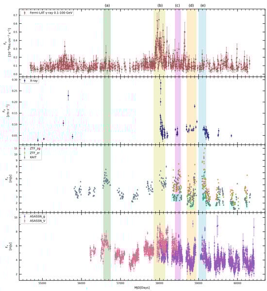
Figure 1.
From top to bottom, the panels exhibit the light curves of -ray of 0.1–100 GeV, X-ray of 0.3–10 keV, optical from KAIT and optical r band and g band from ZTF, optical V band and g band from ASSA-SN, and radio 15 GHz, respectively. Different background colors also represent different periods. The green zone represents period (a) from MJD 56,560 to MJD 56,750, the yellow zone represents period (b) from MJD 57,850 to MJD 58,150, the pink zone represents period (c) from MJD 58,400 to MJD 58,550, the orange zone represents period (d) from MJD 58,700 to MJD 58,950, and the blue zone denotes period (e) from MJD 59,050 to MJD 59,200.
The light curve of OVRO exhibited in the bottom panel of Figure 1 has a general long-term trend due to the superposition of multiple short-term flares. So we use a function of a fifth-degree polynomial as a baseline to depict it. In Section 3, we use the data of radio minus baseline to perform the correlation analysis between radio and other wavelengths to minimize the stacking effect of radio knots.
In order to investigate the variation behavior at different timescales, we select five periods based on the activity states of the optical band. Different periods exhibit different flux states, so that we could study the variation characteristics of this target comprehensively. Epoch (a) represents a medium size flare, epoch (b) shows the most luminous flare, epoch (c) represents the quiescent state with a tiny flare (the peaked flux only doubles the flux at quescent state) at -ray band, epoch (d) represents a stable state, and epoch (e) represents the decaying phase of the flare.
3. Correlation Analysis
3.1. Analysis Methods
Investigating the correlation of multiwavelength is important to study locations in the emission region [34]. Discrete correlation function (DCF; [35]) is one of the most commonly used methods to calculate the correlation of unevenly sampled light curves. However, Max-Moerbeck et al. [36] have mentioned that the value of the DCF can exceed the range of , which is not well limited. Welsh [37] proposed the LCCF method by using only the overlapping samplings to calculate the average and standard deviations. This restricts the correlation values bounded to , as a consequence of the Cauchy–Schwarz inequality. The LCCF is defined as
where and denote the quantities observed at and , N counts pairs where ( is the lag bin), and are averaged values for data in N pairs, and and are the standard deviations, correspondingly.
Additionally, the previous studies have revealed that the LCCF is more efficient than the DCF in picking up the correlation signals [36]. Thus, we use the LCCF to study correlations between light curves at different bands. To estimate the significance of the time lag, we applied the Monte Carlo (MC) method. Our MC simulation procedure refers to both Cohen et al. [38] and Max-Moerbeck et al. [36]. First, we simulate artificial light curves with a time bin of 1 day by the method described in [39] (TK95). For TXS 0506+056, the slopes of the power spectral density (PSD) of -ray, KAIT merged r band of ZTF, V band of ASAS-SN, and radio light curves are , , , and , respectively. Secondly, we computed LCCFs between simulated light curves and observed light curves at each lag bin to obtain the correlation distribution. Due to correlation coefficients for each lag time, 0.01% precision can be achieved for the significance estimation. We obtain the , , and confidence levels corresponding to the , , and chance probabilities.
If a correlation peak exceeds the level, we consider it as significant. We calculate the location of the peak of LCCF () and the centroid lag around the peak of the LCCF () of the significant peaks. is defined as , where is the correlation coefficient satisfying > 0.8 LCCF () [40]. The error ranges of both and are calculated by using the FR/RSS method [41].
3.2. Time Lag and Relative Distance
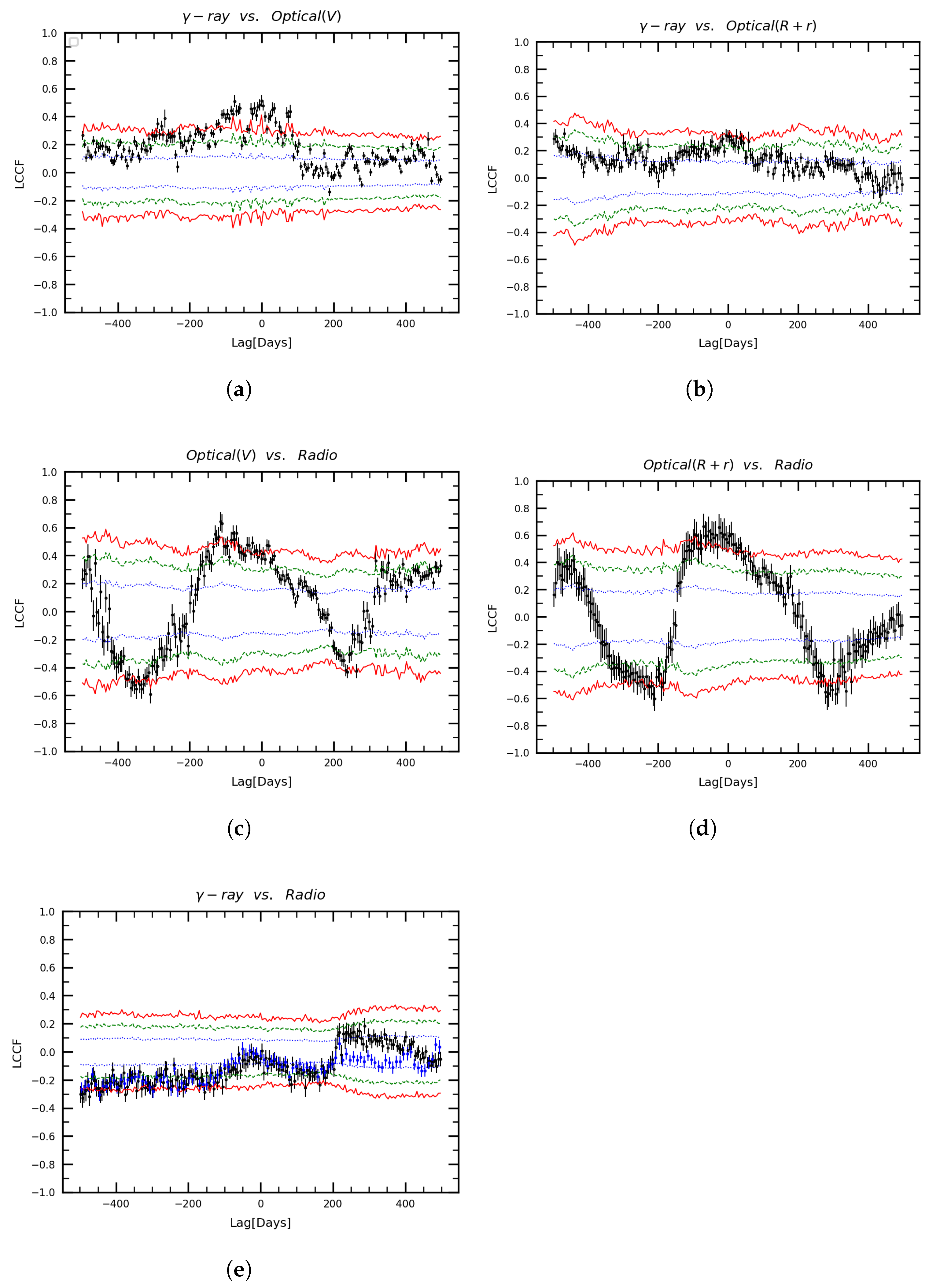
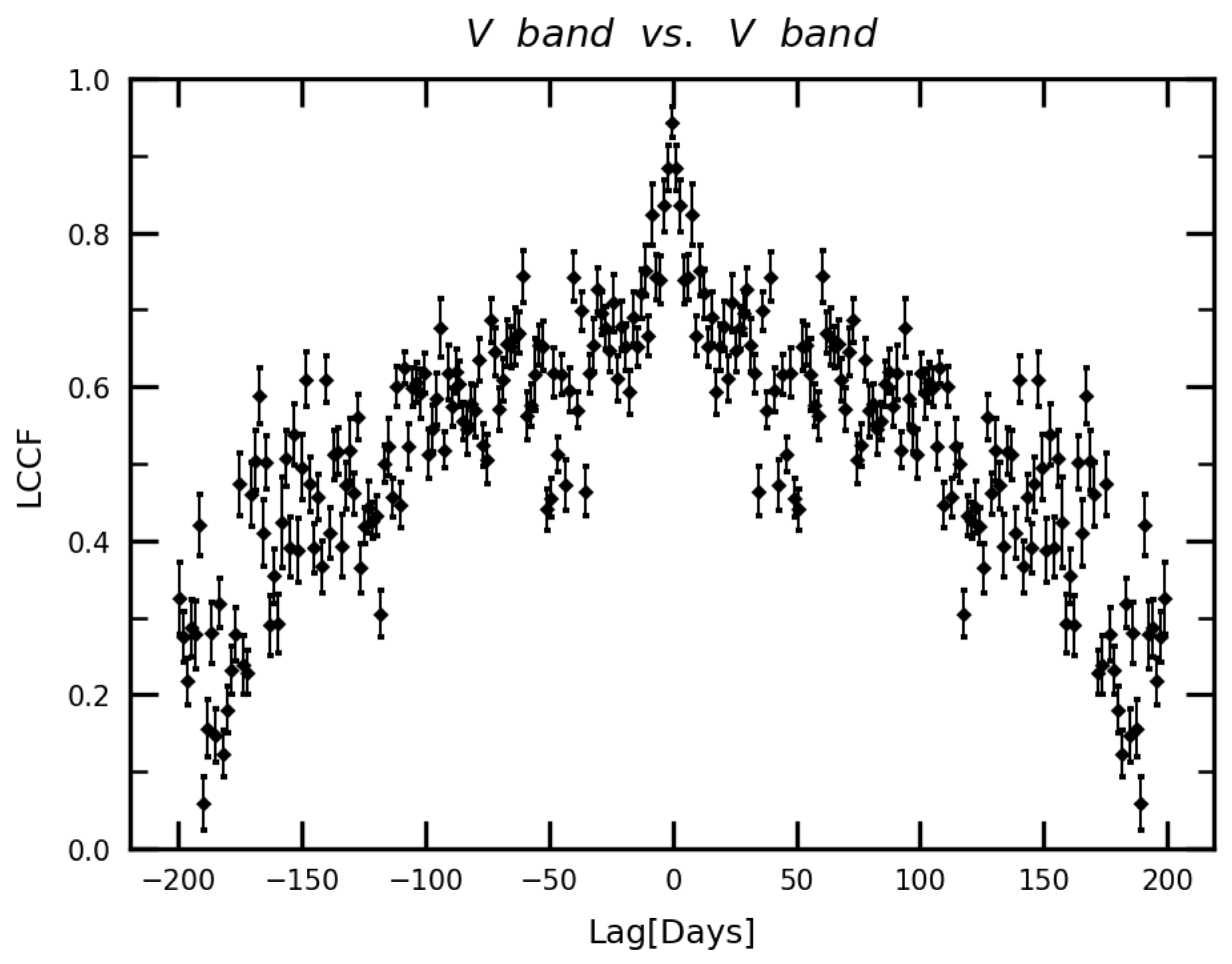
Based on the above methods, we compute the LCCF among the multiwavelength light curves, and the results are plotted in Table 1. To avoid spurious signals caused by the long-term trend of the OVRO light curve, we do not consider radio data after MJD 58,000. In Figure 2a,c,d, the most significant peaks of LCCFs are beyond the 3 significance level. As shown in Figure 2e, a peak appears at about 250 days, with the significance only achieving the 1.5 level. The signal is most probably spurious, which appears mainly because some flares of radio may have led the uncorrelated gamma-ray flare by about 200 days. After we ignore two -ray flares, the LCCF peak is significantly reduced, as evident by the blue dots in the panel. Figure 2a,b shows that the time lags of the -ray versus optical V band and band are approximately zero within uncertainty. This suggests that the emission of -ray and optical bands is most probably from the same region. There are some irregular small peaks around zero day, which is probably caused by the very short-term flares at the V band light curve. The self-LCCF of the ASAS-SN V band is plotted in Figure 3. We observe that the main peak at zero lag does not show a smooth profile but has many small peaks stacking on either side of it. The case is similar to that in Figure 2a. So it indicates that the small peaks around zero day are related to the variability at short time scales. Figure 2c and Figure 2d show the correlation between the optical V and bands versus radio band, respectively. It is notable that the correlation between the radio and band has the LCCF peak exceeding 3 level. Furthermore, the LCCF peaks of the optical V and radio case are beyond the 3 level. However, the centroid time lags of these two cases have discrepancies of about 50 days. Considering the flux errors and data quality, we tend to believe that the lag signal of optical versus radio is more reliable than the optical V-band versus radio case. The short-term scale fluctuations produce the spurious signals, which bias the centroid lag in Figure 2c. Considering that both V and r bands are at optical bands, their emission regions should be the same.

Table 1.
Time Lags and Relative Distances.
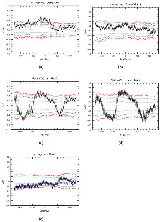
Figure 2.
The LCCF analysis results between different wavebands are plotted. The results are denoted by black dots. In panel (e), the blue dots represented the result of -ray light curve deleting two main peaks. Significance levels of 1, 2, and 3 are depicted by the blue dotted line, green dashed line, and red solid line, respectively.

Figure 3.
The self-LCCF of ASAS-SN V band.
The results of time lags are summarized in Table 1.
Utilizing the time lags, we can calculate the relative distance between different emission regions according to the following formula:
where is the apparent velocity in unit of c, is the time lag between the different bands calculated above, denotes the viewing angle between jet axis and observing line of sight, and z is the redshift. For this source, the jet parameters are measured by the MOJAVE project [42]. Its redshift [43]. The apparent velocities have been measured for five features. Jet parameters are derived from variations in radio fluxes and knot features in images, and can vary within a range for different knot observations. Here, we take the fastest feature with [44]. According to the function , we obtain that the viewing angle is for . The larger will lead to smaller . We will adopt to derive the distance, which is a modest estimation for the distance.
The results of , , and are demonstrated in Table 1. We conclude that the -ray emitting region is the same as the V and band emitting region and are upstream of the radio emitting region.
4. Periodicity Analysis
In this work, we used two periodicity analysis methods including the generalized Lomb–Scargle (GLS) [45] and the weighted wavelet Z-transform (WWZ) to study the QPO signals [46].
4.1. The Weighted Wavelet Z-Transform
Fourier transform is an important method for periodicity analysis. It can transform the signal from the time domain to the frequency domain [47]. The wavelet transform is suitable to detect transient periodic fluctuations. However, for the uneven sampled time series, it is affected more by the irregularities of the number and sampling interval. Based on the Morlet wavelet [48], the weighted wavelet Z-transform (WWZ) was proposed by Foster [46].
where the parameter is the normalized weight defined as , and is the measurement error. is the effective number, is the weighted variation of the data, and is the weighted variation of the model function.
In order to show the quasi-periodic oscillation (QPO) and their significance in a more intuitive way, we normalized the WWZ power in each frequency bin. We simulate light curves by adopting the power spectral density (PSD) and the probability distribution function (PDF) from the observed light curve. Then, we study the distribution of power and obtain the significance levels [47].
4.2. Periodicity
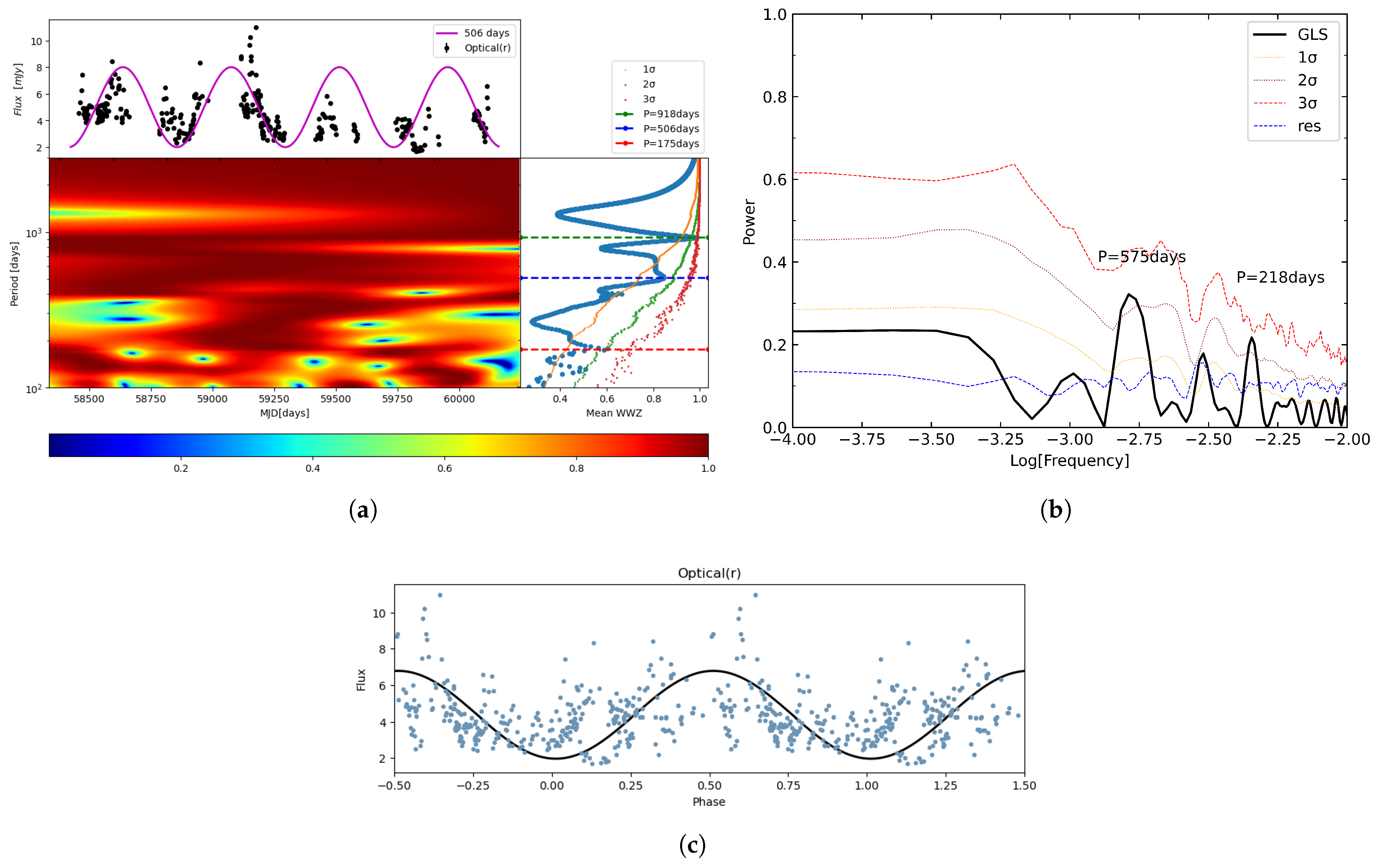
The periodicity analysis result of TXS 0506+056 is plotted in Figure 4. Figure 4a is the result of WWZ analysis of ZTF r-band, which includes three parts. The black dots in the upper left plot represent the light curve of the r-band. The purple solid line represents the fitting result of the sine function with a period of 506 days. The graph in the lower left represents the WWZ periodogram. In the lower right of the panel, the blue line represents the curve of WWZ power. The orange, green, and red dotted lines represent the 1, 2, and 3 confidence levels, respectively. The red, blue, and green dotted horizontal lines represent the QPO signals; the corresponding QPO are 175, 506, and 918 days, respectively. Figure 4c represents the result of phase folding of optical data with a period of 506 days.
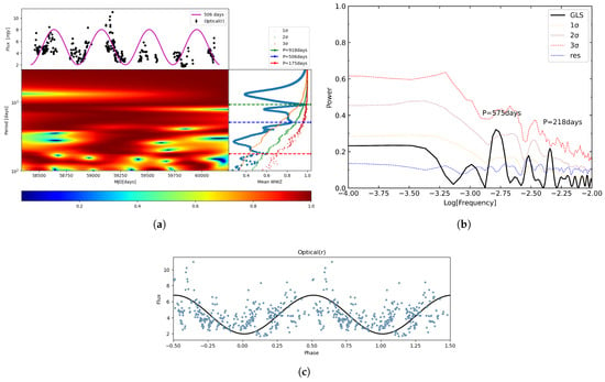
Figure 4.
WWZ and GLS analysis for periodicity. Panel (a) shows the WWZ results, Panel (b) shows the GLS results, and Panel (c) show the phase-fold result. The blue dotted line in the GLS plot is used to check sampling effects.
QPO signal at 918 days has a nominal significance of 3. However, the time range (MJD 58,338 to MJD 60,247) covers only about two cycles. So the QPO of 918 days is not reliable at this stage. Long-term monitoring data are necessary to test this signal. The significance of the QPOs at 175 days and 506 days are over 2 and 1, respectively. The QPO at 506 days seems to exist throughout the observation, while the QPO at 175 days gradually appears and then decays during the observation. We use the full-width-half-maximum (FWHM) to represent the uncertainty of the periods. The results of QPOs in the r band are days and days.
We plot the GLS of ZTF r-band data in Figure 4b. The plot indicates that there are two QPOs at and days with level. With an error, these two QPO signals agree with the QPO results from the WWZ method. The significance of GLS is estimated by the MC procedure. We simulated artificial light curves with even samplings (one day bin). The simulated light curves have the same power spectral density (PSD) and probability distribution function (PDF) as the observed light curve. Then, we perform the GLS for the subsets of simulated light curves, which are filtered with the observing sampling. The significance levels are obtained from the GLS distribution of the random data. By the MC procedure, we can also obtain the residuals of the GLS to demonstrate the spurious signals caused by the sampling effect. We subtract the averaged GLS of the uneven observing sampling data sets from that of the even sampling data sets to obtain the residuals. If there is a peak in the residuals, the corresponding QPO is most likely due to the sampling effect. As indicated in Figure 4b, the GLS peaks at 575 and 201 days have no evident corresponding residual peaks. Thus, the sampling effects can be excluded for these two QPOs. The result of QPOs of this target can support the idea proposed by de Bruijn et al. [9], and the SMBBH may have the hadronic process that produces the neutrino emission.
5. Spectral Variability
The variability exhibited by blazars is a characteristic that merits further investigation. The one-zone leptonic model cannot reproduce the high energy emission of BL Lac objects. For instance, Roychowdhury et al. [49] found that the broad GeV and TeV emission of AP Librae can be explained by the IC process with cosmic microwave background (CMB) photons at kpc scale and with photons from dust disk, respectively. Aharonian et al. [50] found that the high energy and very high energy (VHE) gamma-ray photons show different variation behaviors, suggesting the distinct emission region for these two bands. Here, we use the two-component model and try to explain the behavior of the -ray PI, X-ray HR, optical spectral index, and CI. For most BL Lacs, bumps in the SED can be described with a log-parabola spectrum [51]. In the jet-comoving frame, the log-parabolic function is given by
where b is the curvature index, is the intrinsic frequency, is the intrinsic flux at , and is the intrinsic peak frequency corresponding to the maximum of the SED. Due to the Doppler enhancement, the observed flux can be denoted as , and the observed peak frequency is denoted as , where is the Doppler factor and m is the Doppler factor index. m takes 3 for a jet composed of blobs [1]. Equation (4) can be rewritten in the following form
In the SED of blazars, the low-frequency bump is attributed to synchrotron radiation, and the high-frequency bump in the leptonic model is attributed to the IC radiation. We can express the flux by utilizing the superposition of synchrotron, the SSC, and the EC components. The fluxes for the three components are given by
For the synchrotron process, where B is the magnetic field, and is the Lorentz factor for major electrons. For the SSC process, . For the EC process, , where is the bulk Lorentz factor of the jet and is the frequency of the external radiation field. Thus, we can derive and if is the dominant factor.
5.1. γ-Ray Photon Index
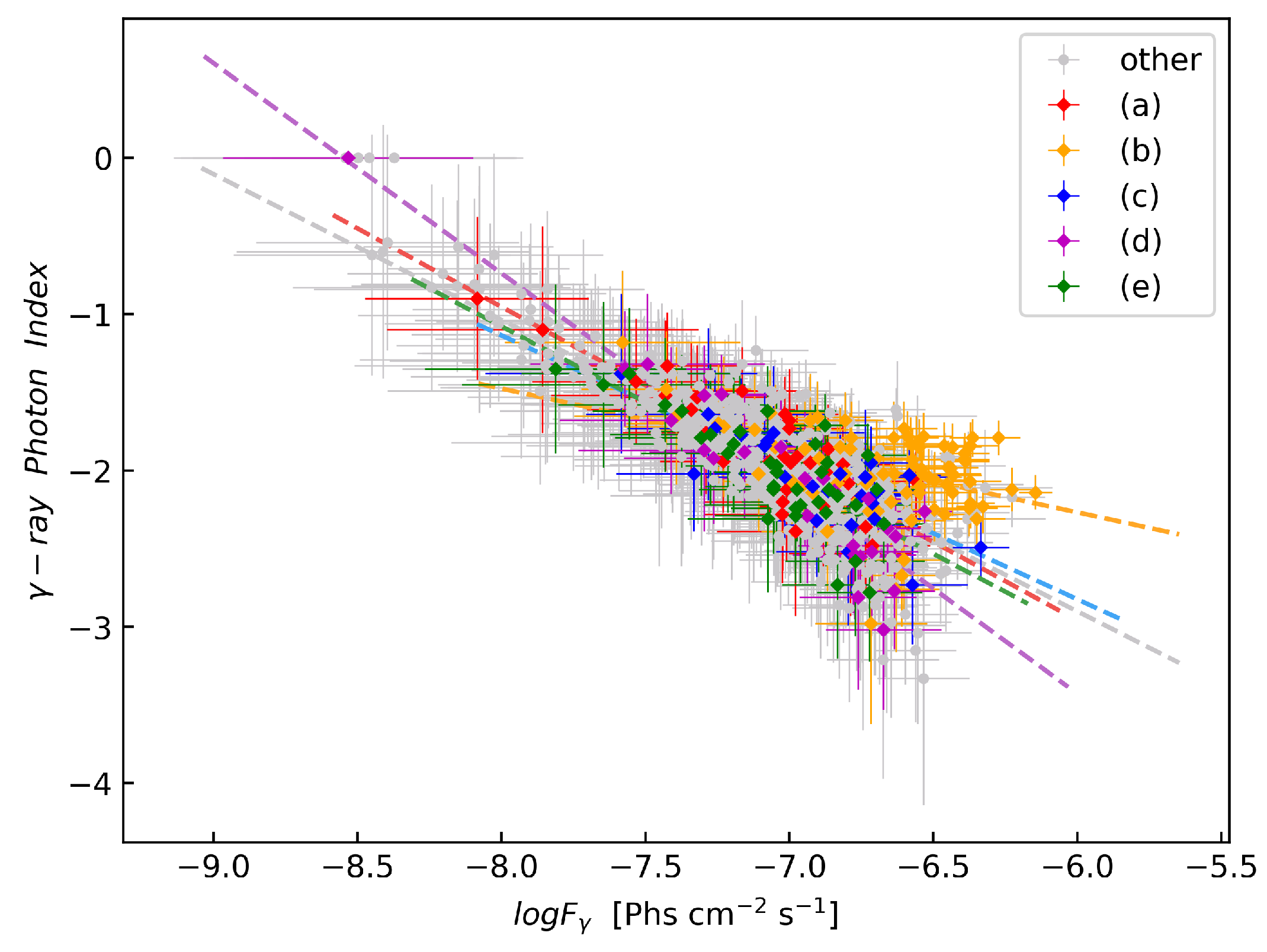
Figure 5 demonstrates the -ray PI versus . We fitted data in all periods via the linear function and performed a correlation study between the PI and the flux by using the Pearson’s coefficient r. The results of the correlation study are reported in Table 2. The last column of the table reports the p-value. In linear regression, if p < 0.05, we consider the linear correlation to be significant.
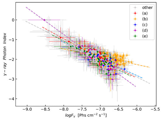
Figure 5.
-ray PI versus is plotted. The symbols corresponding to the epochs are indicated in the upper left legend. Linear fits for PI versus at different epochs are represented by dashed lines.
Table 2.
Linear fitting results of photon index versus logarithmic flux of -ray.
This target presents a softer spectrum during enhanced flux states, namely, a softer when brighter (SWB) trend, which is consistent with Acciari et al. [31]. Epochs (a), (c), (d), and (e) exhibit significant anticorrelations between the photon flux and the PI, since and p-value . Based on the log-parabola function, Wang and Jiang [52] derived the spectral variability slope (k) in the shock-in-jet model
According to the energy range of the Fermi-LAT, which is 0.1–300 GeV, we set to be Hz, which is the most typical frequency of Fermi-LAT. For this target, we take the ranging from to Hz. Chen [53] have studied the curvature index of IC bumps for 48 blazars, where b ranged from 0.032 to 0.48. Taking the range of both b and into Equation (7), we obtain that . So, with only one emission component, Equation (7) cannot explain the SWB behavior of -ray spectral variability. Thus, the one-zone emission model is unable to explain the SWB trend, and the two-component model is a feasible solution. From this point of view, the radiation from BL Lacs may result from the superposition of multiple non-thermal components within the jet. This scenario can also explain the low polarization degrees of BL Lacs [54,55]. The mechanism of the SWB trend at the -ray band for blazars is still an open question [56].
5.2. CI and Optical Spectral Index
Chromatic behavior is also an important manifestation of the spectral variability. Investigating correlations between the CI and the magnitude is useful to study the nature of the micro-variations [57,58,59]. The previous studies on samples of blazars have revealed that the bluer when brighter (BWB) trend is common in BL Lacs, while most FSRQs show a redder when brighter (RWB) trend [60,61,62,63,64]. The underlying physical mechanisms responsible for these trends are related to the emission processes within the jets and the background components like the accretion disc around the central supermassive black hole.
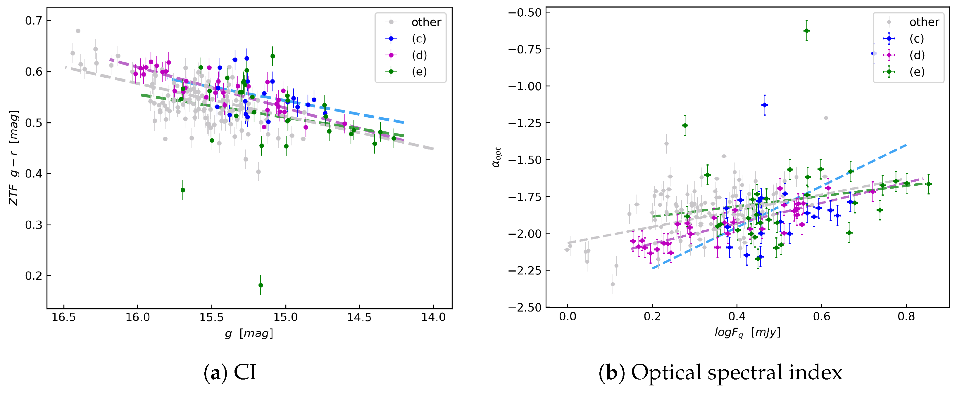
In this work, we pair the magnitudes in the g band and r band with a time bin of less than 1 day and calculate the CI (). The CI () versus g magnitude was shown in Figure 6a. The linear fitting result is demonstrated in Table 3. All epochs show negative correlation between CI and , implying the BWB trend. Especially in epoch (d), the correlation is strong with . A BWB trend may be attributed to shock-in-jet processes, i.e., the shock within the jet accelerates relativistic electrons, leading to the increase in the high-energy electrons. For radiation, the CI tends to be bluer as the jet becomes brighter [65].
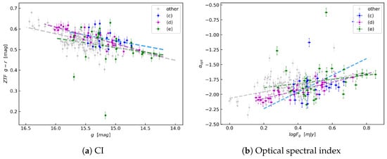
Figure 6.
(a) versus g band magnitude of ZTF. Linear fits for the color indices versus magnitudes are represented by dashed lines. (b) The optical spectral index versus . Linear fits of (c), (d) and (e) are represented by dashed line.
Table 3.
Linear Fitting Results of versus and versus .
The variation in spectral index can reveal the variation mechanism in the quantitative manner. Normally, the optical spectrum can be described by a simple power law
where is the spectral index, and A represents the flux amplitude. We can obtain from the CI via
The optical spectral index versus was plotted in Figure 6b. Compared to the SWB tendency in -ray band, the optical variation shows a harder when brighter (HWB) trend. We performed the linear fitting to study the variation behaviors and the results are listed in Table 3.
To figure out whether the variation is dominated by extrinsic factor (the Doppler factor ) or intrinsic factor (the intrinsic peak frequency ), Wang and Jiang [52] studied the slope of spectral index versus flux by utilizing the log-parabolic model. According to Equation (5), the spectral index can be obtained by
Thus, the spectral index depends on the curvature parameter b, Doppler factor , and intrinsic peak frequency . For further simplification, we take an empirical relation of [52]. The function of log relying on can be derived as
where C is a constant independent of . In the case of the variation modulated by and , the slopes are respectively derived as
They concluded that if the jet component dominates the variation, the process will show a HWB trend whether the variation is modulated by or . TXS 0506+056 is an intermediate synchrotron-peaked blazar, the synchrotron peak frequency Hz. We take , , and Hz; the range of b is , and the range of is . Then, we calculate that the ranges of and are and , respectively. Thus, the BWB variation trend of all epochs can be explained by the modulation of . Only the epoch (e) could also be explained by the variation in Doppler factor. The shock in the jet accelerates the relativistic electron, causing the intrinsic synchrotron peak frequency to shift to higher energy [52].
5.3. X-Ray HR
The correlation between X-ray HR and flux can also help us to understand the spectral variability in the blazar. The X-ray emission may originate from the synchrotron radiation or the IC process. By analyzing the HR behavior, these two radiation mechanisms can be distinguished. Figure 7 shows the X-ray HR versus the logarithmic X-ray flux (0.3–10 keV). In epoch (b), the slope is (Pearson’s r = , p-value = ), indicating a moderate SWB trend. During epoch (c), the slope is (Pearson’s r = , p-value = 0.434), exhibiting a weak SWB behavior. During epoch (d), the slope is , (Pearson’s r = , p-value = 0.098). This epoch exhibits another moderate SWB behavior. During epoch (e), the slope is (Pearson’s r = , p-value = 0.822), indicating an achromatic behavior at the end of the flare.
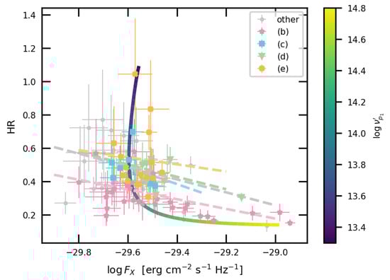
Figure 7.
The plot of X-ray HR versus . Linear fits for these correlations are represented by dashed lines. The theoretical curve of the log-parabolic model is depicted by the solid curve, and the log [Hz] varies from 13.3 to 14.8, denoted by the right color bar. For synchrotron and SSC, the curvatures are and , and the intrinsic fluxes are and .
The X-ray HR is defined as
where corresponds to hard X-ray flux in the energy range of 2∼10 keV, and corresponds to soft X-ray flux in the energy range of 0.3∼2 keV. We use the frequency corresponding to the average value of energy ranges to calculate the fluxes, so , . The average frequency of the total X-ray flux (0.3–10 keV) is . We can obtain by using the rate multiplying the flux-to-rate factor erg cm−2s−1/counts s−1.
We assume that the hard and soft X-ray emission includes both the synchrotron and SSC components, so the observed flux can be expressed by . These two fluxes can be represented by Equation (6). By varying the intrinsic peak frequency , the X-ray HR variation is modeled with a solid line in Figure 7, which is consistent with the overall trend of observed data points. The transition trend could be explained by the fact that the synchrotron component dominance transforms to the SSC component dominance in X-ray. The hardness ratio is higher when the SSC component dominates the X-ray band, while the HR is lower when the synchrotron component dominates. Thus, we can draw the conclusion that the X-ray emission is superposed by the synchrotron and SSC components. The variation mechanism is due to the shift of the synchrotron peak frequency , which is common in the shock-in-jet model. The synchrotron plus EC case can also fit the overall trend of HR with physical parameters. We cannot distinguish these two components at this step.
6. The Flux Correlation Between -Ray and Optical Bands
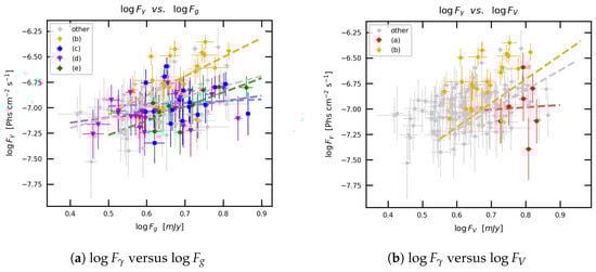
To figure out the emission mechanism at optical and -ray bands, we performed a correlation analysis between observed fluxes of multiwavelength bands. We pair light curves into two groups: -ray and optical V band and -ray and optical g band. We pair the -ray data with optical fluxes with a time uncertainty of 1 day and plot the logarithms of -ray fluxes against logarithms of V and g band fluxes. We perform a linear fitting to the logarithms flux data. Detailed results are demonstrated in Table 4.
Table 4.
Linear fitting results of flux correlation in Figure 8.
The observed fluxes of the synchrotron, SSC, and EC are related to three parameters, i.e., the particle number density , the magnetic field strength B, and the Doppler factor [66].
If the variation of B dominates, the slope in the plot is expected to be 1 for the SSC process. There should be no correlation between optical r band and -ray band for the EC process. Thus, the behavior of epoch (a) and (c) can be explain by the EC process with B dominance. Another possible scenario is that a component dominating the -ray emission during these epochs is not associated with the synchrotron component. However, in other epochs, this component diminishes or even disappears. When the Doppler factor dominates the variation, the SSC process predicts a slope of , and the EC process predicts a slope of . The optical band radiation is generated by the synchrotron, while -ray photons are produced by SSC or EC in the lepton model. For this target, the possible ranges of slopes for the SSC and EC processes are and . Thus, the -ray emission of epochs (d) is dominated by the SSC component, while epoch (e) is dominated by the SSC or EC process. The slope of epoch (b) is obviously higher. Considering the high-energy neutrino emission associated with the -ray flare was detected in epoch (b), the increase in the slope may be caused by the hadronic model. However, the physical mechanism behind it is still an open question.
7. Conclusions
In this work, we conducted a comprehensive multiwavelength analysis of the blazar TXS 0506+056. We collected the multiwavelength light curves of this target, including -ray, X-ray, optical band, and 15 GHz radio. We perform a correlation analysis using the LCCF method, calculating time lags and relative distance among different emission regions. We focused on the spectral variability behaviors at multiwavelength and proposed a theoretical model to explain the variation mechanism behind it. The principal findings of this work are summarized as follows:
- Using the LCCF, we found that the correlation between -ray versus optical and optical versus radio band are beyond the 3 level. We calculated time lags between different wavebands. The result of relative distance suggests that the -rays and optical band roughly share the same emission regions, both located upstream of the radio band.
- Using both the WWZ and GLS methods, we analyzed the QPOs in the optical r bands. We found two weak QPOs at days and days from the WWZ method. The GLS results are consistent with the WWZ results within the error range. These findings support that the QPO are possibly due to the jet precession driven by a SMBBH.
- We conducted an analysis of the spectral index variations across the multiwavelength. The -ray PI exhibits a SWB behavior, and the optical spectral index shows a HWB trend. This could be explained that the optical emissions are mainly of synchrotron radiation, while the -ray emissions may originate from multiple components. The trend of X-ray HR shows a transition. It could be explained that the X-ray emission is composed of synchrotron and IC components, and the trend transition is due to the the shift in peak frequency.
- For this target, by analyzing the flux correlations, we obtain that the -ray emission is dominated by different processes at different epochs. The EC process with B dominance and a component not associated with the synchrotron component can both explain the non-correlation between the -ray and optical fluxes. During the flare associated with the neutrino event, there are excess -ray emissions compared with flares at other epochs. This suggests that the extra hadronic process also contributes to the -ray radiation.
Author Contributions
Writing—original draft preparation, X.M.; writing—review and editing, Y.J. All authors have read and agreed to the published version of the manuscript.
Funding
This research received no external funding.
Data Availability Statement
This research has made use of data from the OVRO 40-m monitoring program [19]. This monitoring program has been supported by NSF grants AST-0808050 and AST-1109911, and is currently supported by NSF grant AST-2407603 and AST-2407604. It has also been supported by NASA grants NNX08AW31G, NNX11A043G, and NNX14AQ89G.
Conflicts of Interest
The authors declare no conflicts of interest.
Notes
| 1 | https://fermi.gsfc.nasa.gov/ssc/ (accessed on 11 May 2024) |
| 2 | http://www.swift.psu.edu/monitoring (accessed on 11 May 2024) |
| 3 | https://asas-sn.osu.edu/(accessed on 11 May 2024) |
| 4 | http://www.astro.caltech.edu/ovroblazars/(accessed on 1 September 2018) |
References
- Urry, C.M.; Padovani, P. Unified schemes for radio-loud active galactic nuclei. Publ. Astron. Soc. Pac. 1995, 107, 803. [Google Scholar] [CrossRef]
- Stickel, M.; Fried, J.W.; Kuehr, H.; Padovani, P.; Urry, C.M. The complete sample of 1 Jansky BL Lacertae objects. I. Summary properties. Astrophys. J. 1991, 374, 431. [Google Scholar] [CrossRef]
- Weymann, R.J.; Morris, S.L.; Foltz, C.B.; Hewett, P.C. Comparisons of the Emission-Line and Continuum Properties of Broad Absorption Line and Normal Quasi-stellar Objects. Astrophys. J. 1991, 373, 23–53. [Google Scholar] [CrossRef]
- Böttcher, M.; Reimer, A.; Sweeney, K.; Prakash, A. Leptonic and hadronic modeling offermi-detected blazars. Astrophys. J. 2013, 768, 54. [Google Scholar] [CrossRef]
- Sikora, M.; Begelman, M.C.; Rees, M.J. Comptonization of diffuse ambient radiation by a relativistic jet: The source of gamma rays from blazars? Astrophys. J. 1994, 421, 153. [Google Scholar] [CrossRef]
- Mannheim, K. The proton blazar. Astron. Astrophys. 1993, 269, 67–76. [Google Scholar] [CrossRef]
- Cerruti, M.; Zech, A.; Boisson, C.; Inoue, S. A hadronic origin for ultra-high-frequency-peaked BL Lac objects. Mon. Not. R. Astron. Soc. 2015, 448, 910–927. [Google Scholar] [CrossRef]
- Padovani, P.; Giommi, P.; Resconi, E.; Glauch, T.; Arsioli, B.; Sahakyan, N.; Huber, M. Dissecting the region around IceCube-170922A: The blazar TXS 0506+056 as the first cosmic neutrino source. Mon. Not. R. Astron. Soc. 2018, 480, 192–203. [Google Scholar] [CrossRef]
- De Bruijn, O.; Bartos, I.; Biermann, P.L.; Tjus, J.B. Recurrent Neutrino Emission from Supermassive Black Hole Mergers. Astrophys. J. Lett. 2020, 905, L13. [Google Scholar] [CrossRef]
- Véron-Cetty, M.P.; Véron, P. A catalogue of quasars and active nuclei: 12th edition. Astron. Astrophys. 2006, 455, 773–777. [Google Scholar] [CrossRef]
- Healey, S.E.; Romani, R.W.; Taylor, G.B.; Sadler, E.M.; Ricci, R.; Murphy, T.; Ulvestad, J.S.; Winn, J.N. CRATES: An All-Sky Survey of Flat-Spectrum Radio Sources. Astrophys. J. Suppl. Ser. 2007, 171, 61–71. [Google Scholar] [CrossRef]
- Padovani, P.; Oikonomou, F.; Petropoulou, M.; Giommi, P.; Resconi, E. TXS 0506+056, the first cosmic neutrino source, is not a BL Lac. Mon. Not. R. Astron. Soc. Lett. 2019, 484, L104–L108. [Google Scholar] [CrossRef]
- Abdollahi, S.; Ajello, M.; Baldini, L.; Ballet, J.; Bastieri, D.; Becerra Gonzalez, J.; Bellazzini, R.; Berretta, A.; Bissaldi, E.; Bonino, R.; et al. The Fermi-LAT Lightcurve Repository. Astrophys. J. Suppl. Ser. 2023, 265, 31. [Google Scholar] [CrossRef]
- Stroh, M.C.; Falcone, A.D. Swift X-ray telescope monitoring of fermi-lat gamma-ray sources of interest. Astrophys. J. Suppl. Ser. 2013, 207, 28. [Google Scholar] [CrossRef]
- Shappee, B.J.; Prieto, J.L.; Grupe, D.; Kochanek, C.S.; Stanek, K.Z.; Rosa, G.D.; Mathur, S.; Zu, Y.; Peterson, B.M.; Pogge, R.W.; et al. The man behind the curtain: X-rays drive the UV through nir variability in the 2013 active galactic nucleus outburst in ngc 2617. Astrophys. J. 2014, 788, 48. [Google Scholar] [CrossRef]
- Li, W.; Filippenko, A.V.; Chornock, R.; Jha, S. The Katzman Automatic Imaging Telescope Gamma-Ray Burst Alert System, and Observations of GRB 020813. Publ. Astron. Soc. Pac. 2003, 115, 844. [Google Scholar] [CrossRef]
- Masci, F.J.; Laher, R.R.; Rusholme, B.; Shupe, D.L.; Groom, S.; Surace, J.; Jackson, E.; Monkewitz, S.; Beck, R.; Flynn, D.; et al. The Zwicky Transient Facility: Data Processing, Products, and Archive. Publ. Astron. Soc. Pac. 2018, 131, 018003. [Google Scholar] [CrossRef]
- Bellm, E.C.; Kulkarni, S.R.; Graham, M.J.; Dekany, R.; Smith, R.M.; Riddle, R.; Masci, F.J.; Helou, G.; Prince, T.A.; Adams, S.M.; et al. The Zwicky Transient Facility: System Overview, Performance, and First Results. Publ. Astron. Soc. Pac. 2018, 131, 018002. [Google Scholar] [CrossRef]
- Richards, J.L.; Max-Moerbeck, W.; Pavlidou, V.; King, O.G.; Pearson, T.J.; Readhead, A.C.S.; Reeves, R.; Shepherd, M.C.; Stevenson, M.A.; Weintraub, L.C.; et al. Blazars in the Fermi Era: The OVRO 40 m Telescope Monitoring Program. Astrophys. J. Suppl. Ser. 2011, 194, 29. [Google Scholar] [CrossRef]
- Ballet, J.; Burnett, T.H.; Digel, S.W.; Lott, B. Fermi Large Area Telescope Fourth Source Catalog Data Release 2. arXiv 2020. [Google Scholar] [CrossRef]
- Atwood, W.; Albert, A.; Baldini, L.; Tinivella, M.; Bregeon, J.; Pesce-Rollins, M.; Sgrò, C.; Bruel, P.; Charles, E.; Drlica-Wagner, A.; et al. Pass 8: Toward the Full Realization of the Fermi-LAT Scientific Potential. arXiv 2013. [Google Scholar] [CrossRef]
- Bruel, P.; Burnett, T.H.; Digel, S.W.; Johannesson, G.; Omodei, N.; Wood, M. Fermi-LAT improved Pass~8 event selection. arXiv 2018. [Google Scholar] [CrossRef]
- Mattox, J.R.; Bertsch, D.L.; Chiang, J.; Dingus, B.L.; Digel, S.; Esposito, J.; Fierro, J.M.; Hartman, R.C.; Hunter, S.D.; Kanbach, G.; et al. The Likelihood Analysis of EGRET Data. Astrophys. J. 1996, 461, 396. [Google Scholar] [CrossRef]
- Gehrels, N.; Chincarini, G.; Giommi, P.; Mason, K.O.; Nousek, J.A.; Wells, A.A.; White, N.E.; Barthelmy, S.D.; Burrows, D.N.; Cominsky, L.R.; et al. The Swift Gamma-Ray Burst Mission. Astrophys. J. 2004, 611, 1005–1020. [Google Scholar] [CrossRef]
- Burrows, D.N.; Hill, J.E.; Nousek, J.A.; Kennea, J.A.; Wells, A.; Osborne, J.P.; Abbey, A.F.; Beardmore, A.; Mukerjee, K.; Short, A.D.T.; et al. The Swift X-Ray Telescope. Space Sci. Rev. 2005, 120, 165–195. [Google Scholar] [CrossRef]
- Arnaud, K.A. XSPEC: The First Ten Years. In Astronomical Data Analysis Software and Systems V; ASP Conference Series; Jacoby, G.H., Barnes, J., Eds.; Astronomical Society of the Pacific: San Francisco, CA, USA, 1996; Volume 101, p. 17. Available online: https://adsabs.harvard.edu/full/1996ASPC..101...17A (accessed on 19 June 2025).
- Kalberla, P.M.W.; Burton, W.B.; Hartmann, D.; Arnal, E.M.; Bajaja, E.; Morras, R.; Pöppel, W.G.L. The Leiden/Argentine/Bonn (LAB) Survey of Galactic HI. Final data release of the combined LDS and IAR surveys with improved stray-radiation corrections. Astron. Astrophys. 2005, 440, 775–782. [Google Scholar] [CrossRef]
- HI4PI Collaboration; Ben Bekhti, N.; Flöer, L.; Keller, R.; Kerp, J.; Lenz, D.; Winkel, B.; Bailin, J.; Calabretta, M.R.; Dedes, L.; et al. HI4PI: A full-sky H I survey based on EBHIS and GASS. Astron. Astrophys. 2016, 594, A116. [Google Scholar] [CrossRef]
- Kochanek, C.S.; Shappee, B.J.; Stanek, K.Z.; Holoien, T.W.S.; Thompson, T.A.; Prieto, J.L.; Dong, S.; Shields, J.V.; Will, D.; Britt, C.; et al. The All-Sky Automated Survey for Supernovae (ASAS-SN) Light Curve Server v1.0. Publ. Astron. Soc. Pac. 2017, 129, 104502. [Google Scholar] [CrossRef]
- Yuk, H.; Dai, X.; Jayasinghe, T.; Fu, H.; Mishra, H.D.; Kochanek, C.S.; Shappee, B.J.; Stanek, K. Variability Selected Active Galactic Nuclei from ASAS-SN Survey: Constraining the Low Luminosity AGN Population. Astrophys. J. 2022, 930, 110. [Google Scholar] [CrossRef]
- Acciari, V.A.; Aniello, T.; Ansoldi, S.; Antonelli, L.A.; Arbet Engels, A.; Artero, M.; Asano, K.; Baack, D.; Babić, A.; Baquero, A.; et al. Investigating the Blazar TXS 0506+056 through Sharp Multiwavelength Eyes During 2017–2019. Astrophys. J. 2022, 927, 197. [Google Scholar] [CrossRef]
- IceCube Collaboration; Achterberg, A.; Ackermann, M.; Adams, J.; Ahrens, J.; Andeen, K.; Atlee, D.W.; Baccus, J.; Bahcall, J.N.; Bai, X.; et al. First year performance of the IceCube neutrino telescope. Astropart. Phys. 2006, 26, 155–173. [Google Scholar] [CrossRef]
- Hovatta, T.; Lindfors, E.; Kiehlmann, S.; Max-Moerbeck, W.; Hodges, M.; Liodakis, I.; Lähteemäki, A.; Pearson, T.J.; Readhead, A.C.S.; Reeves, R.A.; et al. Association of IceCube neutrinos with radio sources observed at Owens Valley and Metsähovi Radio Observatories. Astron. Astrophys. 2021, 650, A83. [Google Scholar] [CrossRef]
- Wang, Y.F.; Jiang, Y.G. A Comprehensive Study on the Variation Phenomena of AO 0235+164. Astrophys. J. 2020, 902, 41. [Google Scholar] [CrossRef]
- Edelson, R.A.; Krolik, J.H. The Discrete Correlation Function: A New Method for Analyzing Unevenly Sampled Variability Data. Astrophys. J. 1988, 333, 646. [Google Scholar] [CrossRef]
- Max-Moerbeck, W.; Richards, J.L.; Hovatta, T.; Pavlidou, V.; Pearson, T.J.; Readhead, A.C.S. A method for the estimation of the significance of cross-correlations in unevenly sampled red-noise time series. Mon. Not. R. Astron. Soc. 2014, 445, 437–459. [Google Scholar] [CrossRef]
- Welsh, W.F. On the Reliability of Cross-Correlation Function Lag Determinations in Active Galactic Nuclei. Publ. Astron. Soc. Pac. 1999, 111, 1347–1366. [Google Scholar] [CrossRef]
- Cohen, D.P.; Romani, R.W.; Filippenko, A.V.; Cenko, S.B.; Lott, B.; Zheng, W.; Li, W. Temporal correlations between optical and gamma-ray activity in blazars. Astrophys. J. 2014, 797, 137. [Google Scholar] [CrossRef]
- Timmer, J.; König, M. On generating power law noise. Astron. Astrophys. 1995, 300, 707. [Google Scholar]
- Shao, X.; Jiang, Y.; Chen, X. Curvature-induced polarization and spectral index behavior for PKS 1502+106. Astrophys. J. 2019, 884, 15. [Google Scholar] [CrossRef]
- Peterson, B.; Wanders, I.; Horne, K.; Collier, S.; Alexander, T.; Kaspi, S.; Maoz, D. On Uncertainties in Cross-Correlation Lags and the Reality of Wavelength-dependent Continuum Lags in Active Galactic Nuclei. Publ. Astron. Soc. Pac. 1998, 110, 660–670. [Google Scholar] [CrossRef]
- Pushkarev, A.B.; Hovatta, T.; Kovalev, Y.Y.; Lister, M.L.; Lobanov, A.P.; Savolainen, T.; Zensus, J.A. MOJAVE: Monitoring of Jets in Active galactic nuclei with VLBA Experiments: IX. Nuclear opacity. Astron. Astrophys. 2012, 545, A113. [Google Scholar] [CrossRef]
- Paiano, S.; Falomo, R.; Treves, A.; Scarpa, R. The Redshift of the BL Lac Object TXS 0506+056. Astrophys. J. Lett. 2018, 854, L32. [Google Scholar] [CrossRef]
- Lister, M.L.; Homan, D.C.; Kellermann, K.I.; Kovalev, Y.Y.; Pushkarev, A.B.; Ros, E.; Savolainen, T. Monitoring of Jets in Active Galactic Nuclei with VLBA Experiments. XVIII. Kinematics and Inner Jet Evolution of Bright Radio-loud Active Galaxies. Astrophys. J. 2021, 923, 30. [Google Scholar] [CrossRef]
- Zechmeister, M.; Kürster, M. The generalised Lomb-Scargle periodogram-a new formalism for the floating-mean and Keplerian periodograms. Astron. Astrophys. 2009, 496, 577–584. [Google Scholar] [CrossRef]
- Foster, G. Wavelets for period analysis of unevenly sampled time series. Astron. J. 1996, 112, 1709–1729. [Google Scholar] [CrossRef]
- Chen, Z.H.; Jiang, Y. Quasi-periodic oscillation analysis for a sample of blazars at the optical band. Astron. Astrophys. 2024, 689, A35. [Google Scholar] [CrossRef]
- Grossmann, A.; Morlet, J. Decomposition of hardy functions into square integrable wavelets of constant shape. Siam J. Math. Anal. 1984, 15, 723–736. [Google Scholar] [CrossRef]
- Roychowdhury, A.; Meyer, E.T.; Georganopoulos, M.; Breiding, P.; Petropoulou, M. Circumnuclear Dust in AP Librae and the source of its VHE emission. Astrophys. J. 2022, 924, 57. [Google Scholar] [CrossRef]
- Aharonian, F.; Benkhali, F.A.; Aschersleben, J.; Ashkar, H.; Backes, M.; Martins, V.B.; Barnard, J.; Batzofin, R.; Becherini, Y.; Berge, D.; et al. The vanishing of the primary emission region in PKS 1510–089. Astrophys. J. Lett. 2023, 952, L38. [Google Scholar] [CrossRef]
- Tramacere, A.; Giommi, P.; Massaro, E.; Perri, M.; Nesci, R.; Colafrancesco, S.; Tagliaferri, G.; Chincarini, G.; Falcone, A.; Burrows, D.N.; et al. SWIFT observations of TeV BL Lacertae objects. Astron. Astrophys. 2007, 467, 501–508. [Google Scholar] [CrossRef]
- Wang, C.Z.; Jiang, Y.G. Revealing the Variation Mechanism of ON 231 via the Two-component Shock-in-jet Model. Astrophys. J. 2024, 966, 65. [Google Scholar] [CrossRef]
- Chen, L. Curvature of the spectral energy distributions of blazars. Astrophys. J. 2014, 788, 179. [Google Scholar] [CrossRef]
- Kiehlmann, S.; Blinov, D.; Liodakis, I.; Pavlidou, V.; Readhead, A.; Angelakis, E.; Casadio, C.; Hovatta, T.; Kylafis, N.; Mahabal, A.; et al. The time-dependent distribution of optical polarization angle changes in blazars. Mon. Not. R. Astron. Soc. 2021, 507, 225–243. [Google Scholar] [CrossRef]
- Blinov, D.; Kiehlmann, S.; Pavlidou, V.; Panopoulou, G.; Skalidis, R.; Angelakis, E.; Casadio, C.; Einoder, E.; Hovatta, T.; Kokolakis, K.; et al. RoboPol: AGN polarimetric monitoring data. Mon. Not. R. Astron. Soc. 2021, 501, 3715–3726. [Google Scholar] [CrossRef]
- Deng, J.; Jiang, Y. The Spectral Variation Behavior of Fermi-LAT Blazars. Astrophys. J. 2025, 983, 128. [Google Scholar] [CrossRef]
- Gu, M.F.; Ai, Y. The optical variability of flat-spectrum radio quasars in the SDSS stripe 82 region. Astron. Astrophys. 2011, 528, A95. [Google Scholar] [CrossRef]
- Max-Moerbeck, W.; Hovatta, T.; Richards, J.L.; King, O.G.; Pearson, T.J.; Readhead, A.C.S.; Reeves, R.; Shepherd, M.C.; Stevenson, M.A.; Angelakis, E.; et al. Time correlation between the radio and gamma-ray activity in blazars and the production site of the gamma-ray emission. Mon. Not. R. Astron. Soc. 2014, 445, 428–436. [Google Scholar] [CrossRef]
- Xiong, D.; Zhang, H.; Zhang, X.; Yi, T.; Bai, J.; Wang, F.; Liu, H.; Zheng, Y. Multi-color optical monitoring of MRK 501 from 2010 to 2015. Astrophys. J. Suppl. Ser. 2016, 222, 24. [Google Scholar] [CrossRef]
- Vagnetti, F.; Trevese, D.; Nesci, R. Spectral Slope Variability of BL Lac Objects in the Optical Band. Astrophys. J. 2008, 590, 123. [Google Scholar] [CrossRef]
- Kudryavtseva, N.A.; Gabuzda, D.C.; Aller, M.F.; Aller, H.D. A new method for estimating frequency-dependent core shifts in active galactic nucleus jets. Mon. Not. R. Astron. Soc. 2011, 415, 1631–1637. [Google Scholar] [CrossRef]
- Ikejiri, Y.; Uemura, M.; Sasada, M.; Ito, R.; Yamanaka, M.; Sakimoto, K.; Arai, A.; Fukazawa, Y.; Ohsugi, T.; Kawabata, K.S.; et al. Photopolarimetric Monitoring of Blazars in the Optical and Near-Infrared Bands with the Kanata Telescope. I. Correlations between Flux, Color, and Polarization. Publ. Astron. Soc. Jpn. 2011, 63, 639–675. [Google Scholar] [CrossRef]
- Bonning, E.; Megan Urry, C.; Bailyn, C.; Buxton, M.; Chatterjee, R.; Coppi, P.; Fossati, G.; Isler, J.; Maraschi, L. Smarts optical and infrared monitoring of 12 gamma-ray bright blazars. Astrophys. J. 2012, 756, 13. [Google Scholar] [CrossRef]
- Wierzcholska, A.; Ostrowski, M.; Stawarz, Ł.; Wagner, S.; Hauser, M. Longterm optical monitoring of bright BL Lacertae objects with ATOM: Spectral variability and multiwavelength correlations. Astron. Astrophys. 2014, 573, A69. [Google Scholar] [CrossRef]
- Zibecchi, L.; Andruchow, I.; Marchesini, E.J.; Cellone, S.A.; Combi, J.A. Optical monitoring in southern blazars. Analysis of variability and spectral colour behaviours. Mon. Not. R. Astron. Soc. 2024, 535, 3262–3282. [Google Scholar] [CrossRef]
- Chatterjee, R.; Bailyn, C.D.; Bonning, E.W.; Buxton, M.; Coppi, P.; Fossati, G.; Isler, J.; Maraschi, L.; Urry, C.M. Similarity of the Optical-Infrared and γ-Ray Time Variability of Fermi Blazars. Astrophys. J. 2012, 749, 191. [Google Scholar] [CrossRef]


Disclaimer/Publisher’s Note: The statements, opinions and data contained in all publications are solely those of the individual author(s) and contributor(s) and not of MDPI and/or the editor(s). MDPI and/or the editor(s) disclaim responsibility for any injury to people or property resulting from any ideas, methods, instructions or products referred to in the content. |
© 2025 by the authors. Licensee MDPI, Basel, Switzerland. This article is an open access article distributed under the terms and conditions of the Creative Commons Attribution (CC BY) license (https://creativecommons.org/licenses/by/4.0/).