
From Barthel–Randers–Kropina Geometries to the Accelerating Universe: A Brief Review of Recent Advances in Finslerian Cosmology

 ,
,  ,
,
Abstract
1. Introduction—Early History and Modern Developments
- In the first step, the basic physical/empirical entities are postulated, such as the timelike worldlines for freely falling massive particles, the lightlike worldlines of light rays, and radar echoes between massive particle worldlines. These empirical elements provide enough structure to define a system of coordinates and allow for the construction of a differentiable structure on the spacetime set M, turning it into a smooth manifold.
- The conformal structure is established by requiring that, at each point in spacetime, the set of all possible directions (i.e., tangent vectors) splits into two components when the directions corresponding to massless (lightlike) trajectories are removed. This splitting reflects the causal distinction between future and past. Additionally, in a sufficiently small neighborhood V around the worldline of a massive particle, for any point not lying on the particle’s path, the function that maps p to the product of the radar emission time and reception time , i.e., , must be at least twice differentiable.
- Imposing that through each point in spacetime, and for each timelike direction, there exists one unique timelike (massive) trajectory passing through that point, which results in a projective structure. Each of these trajectories must admit a parametrization such that, in local coordinates near the point, the motion satisfies . This expresses the fact that particles move along straight lines in free fall.
- In the final step, compatibility between the conformal and projective structures is required. In particular, light rays must be special cases of particle geodesics in the limit of zero mass. This determines the metric up to a conformal factor, which leads to a Weyl structure. Through some technical steps, eliminating the second clock effect leads to a Lorentzian structure, i.e., a pseudo-Riemannian manifold.
2. Fundamentals of Finsler Geometry
- (i)
- is on .
- (ii)
- is positively 1-homogeneous: , for all and .
- (iii)
- For each , the Hessian matrix (29) is positive definite on .
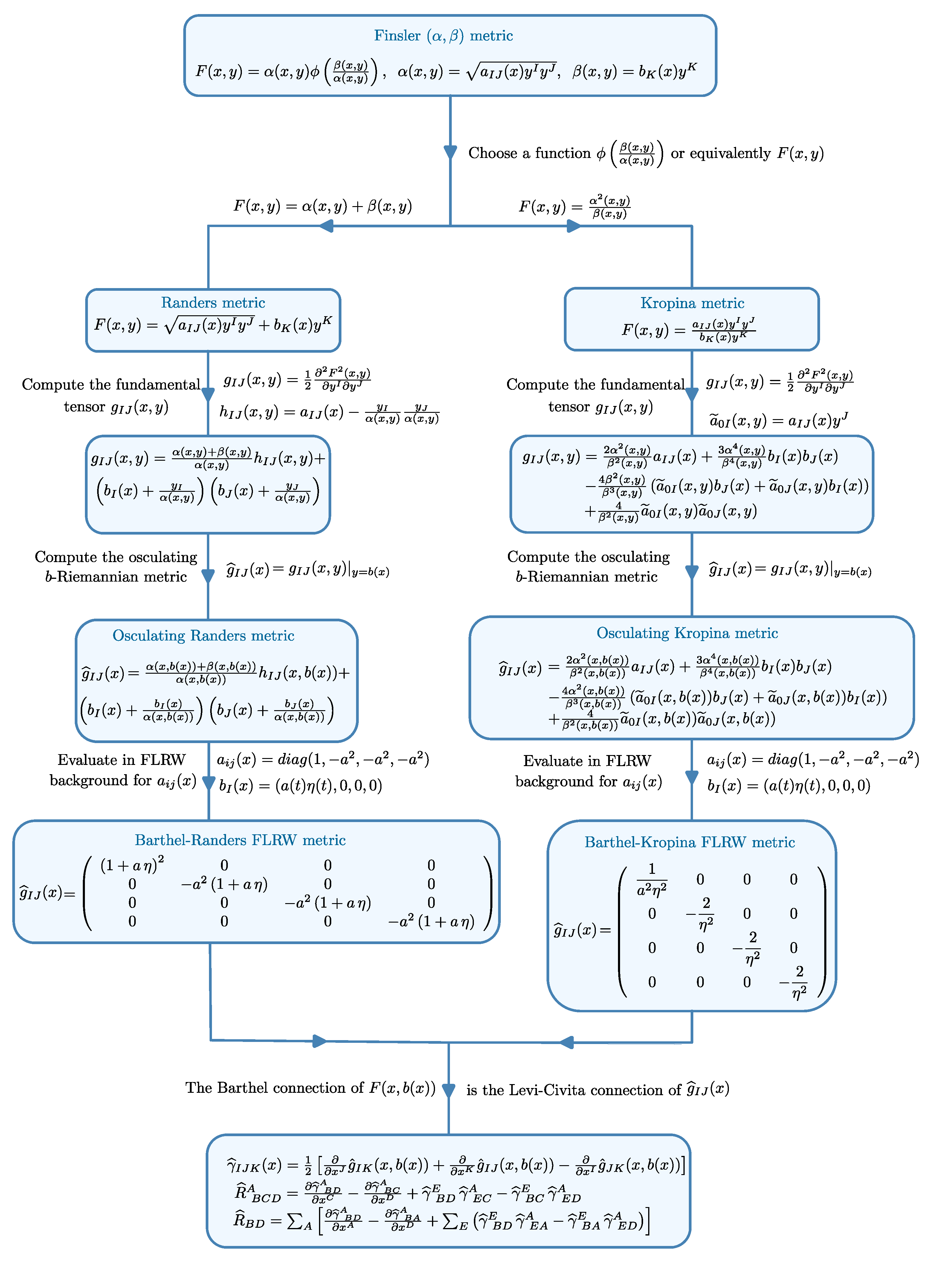
3. Osculating -Type Cosmological Models
3.1. Mathematical Foundations of the Finslerian Cosmologies
3.1.1. Kropina and Geometries
3.1.2. The Barthel Connection
3.1.3. The Y-Osculating Riemann Geometry
- The case of the metrics.
- The curvature tensor.
3.2. Building Cosmological Models in Geometries
- The Universe is homogeneous and isotropic.
- The Riemannian metric is the FLRW metric.
- The Finsler metric depends on only.
- The 1-form b has vanishing space-like components.
- Matter moves along the Hubble flow.
- The matter content of the Universe is a perfect fluid.
- Geometric quantities.
- (iii)
- (iv)
- ;
- (v)
- ;
- (vi)
- Gravitational field equations.
- Flowchart of the algorithmic construction of osculating Barthel-type Finslerian gravitational theories.
3.3. Barthel–Randers Cosmology
- The energy conservation equation.
3.4. Barthel–Kropina Cosmology
- Energy balance equation.
- The general relativistic limit.
3.5. Conformal Barthel–Kropina Cosmology
- The generalized Friedmann equations.
3.6. Thermodynamic Interpretation of the Cosmologies
3.6.1. Irreversible Thermodynamics and Matter Creation
- Particle balance equations.
- The entropy flux.
- The creation pressure.
3.6.2. Application: Particle Creation in Barthel–Randers Cosmology
- Creation pressure in Barthel–Randers cosmology.
- The particle creation rate.
- The matter temperature.
3.6.3. Creation of Exotic Matter
4. Cosmological Implications of Barthel–Randers and Barthel–Kropina Models
4.1. Specific Cosmological Models
- Linear model: .
- Logarithmic model: .
- Exponential model: .
4.2. Methodology and Datasets
- Cosmic Chronometers: In this study, we use the Hubble measurements extracted based on the differential age approach. This technique leverages passively evolving massive galaxies, which formed at redshifts around , enabling a direct and model-independent determination of the Hubble parameter using the relationship . This method significantly reduces the reliance on astrophysical assumptions [163]. For our analysis, we use 15 Hubble measurements selected from the 31 Hubble measurements, which cover a redshift range from [164,165,166]. We use the likelihood function provided by Moresco in his GitLab repository3 which uses the full covariance matrix, accounting for both statistical and systematic uncertainties [167,168].
- Type Ia Supernova: We also use the Pantheon+ dataset without the SHOES calibration, which consists of 1701 light curves from 1550 Type Ia Supernovae (SNe Ia) covering a redshift range of [169]. To analyze this data, we adopt the likelihood function described in [170], which incorporates the total covariance matrix, , which includes both statistical () and systematic () uncertainties [171]. The likelihood function is given by where represents the residual vector, defined as the difference between the observed and theoretical distance moduli: , where . Here, is the inverse of the total covariance matrix. The model-predicted distance modulus is calculated as where the luminosity distance in a flat FLRW Universe is given by Here, c is the speed of light, and is the Hubble parameter. This formulation highlights the degeneracy between the nuisance parameter and the Hubble constant .
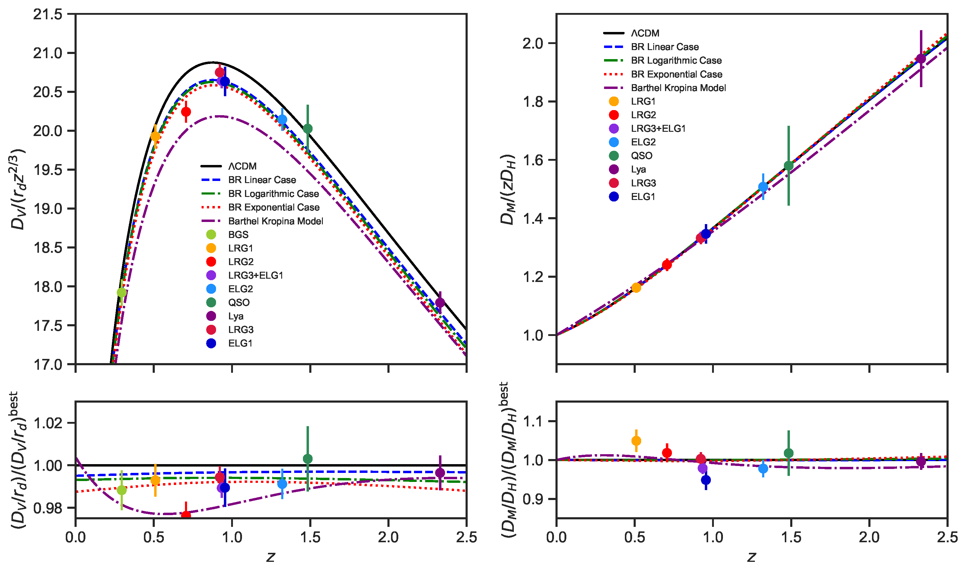
- Baryon Acoustic Oscillation: In our analysis, we also include the 13 recent Baryon Acoustic Oscillation (BAO) measurements from the Dark Energy Spectroscopic Instrument (DESI) Data Release 2 (DR2) [172]. These measurements cover a redshift range of . They were obtained from observations of the Bright Galaxy Sample (BGS), Luminous Red Galaxies (LRG1, LRG2, LRG3), Emission Line Galaxies (ELG1 and ELG2), Quasars (QSO), and Lyman- tracers4. The measurements are reported using three distance indicators: the Hubble distance , the comoving angular diameter distance , and the volume-averaged distance . To compare these with cosmological models, we compute the ratios , , and , where represents the sound horizon at the drag epoch, occurring around redshift . In a flat CDM model, Mpc [72]. However, in this study, we treat as a free parameter, allowing late-time observations to constrain the corresponding model parameters [173,174,175,176,177]. The chi-squared statistic for the BAO measurements is given by where and denote the vectors of theoretical predictions and observed measurements, respectively, and is the associated covariance matrix5.
Convergence Test
- Gelman–Rubin Statistic
- Convergence of Chains and Trace Plots
5. Comparing Barthel–Randers, Barthel–Kropina and CDM Models
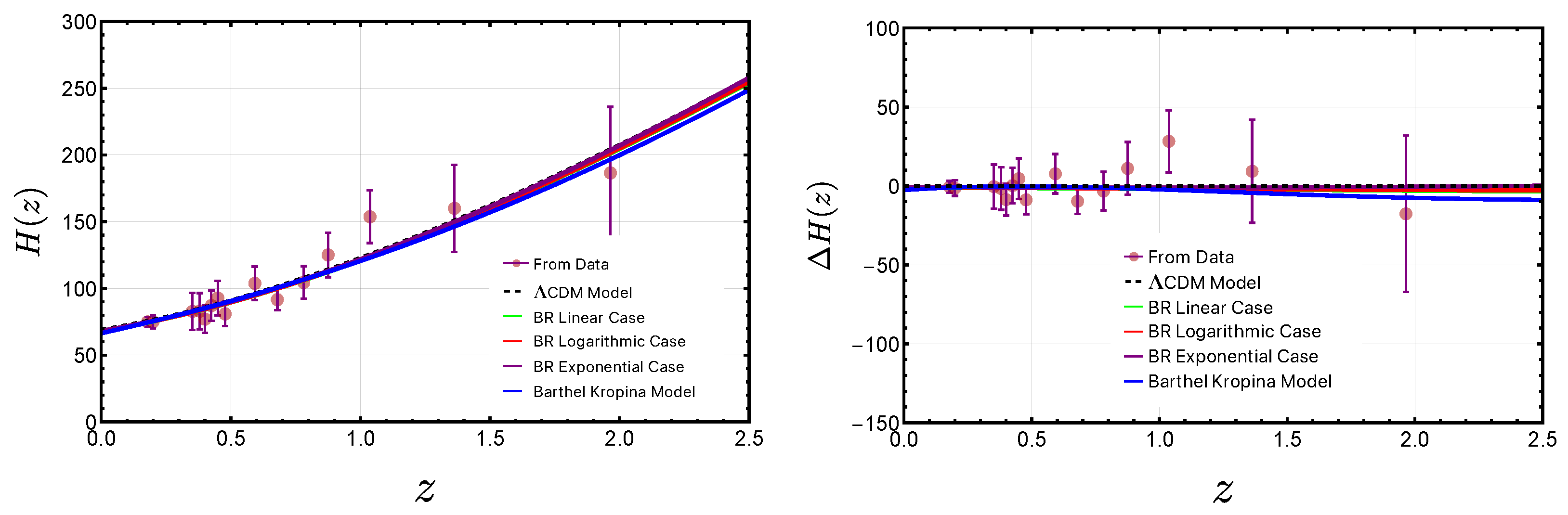
5.1. Evolution of the Hubble Parameter, Hubble Residual, and BAO Distance Scales
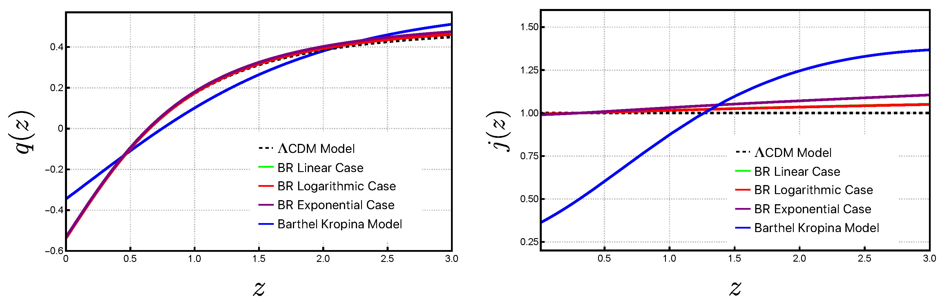
5.2. Cosmographic Analysis of Barthel–Randers and Barthel–Kropina Models
Deceleration Parameter and Jerk Parameter
5.3. Statistical Assessment of Barthel–Randers and Barthel–Kropina Models
5.4. Goodness of Fit
5.4.1. Model Comparison Using AIC and BIC
5.4.2. Relative Comparison: AIC and BIC
- : Comparable support.
- : Considerably less support.
- : Strongly disfavored.
- : Weak evidence against the model.
- : Moderate evidence against the model.
- : Strong evidence against the model.
5.4.3. p-Value Statistics
6. Summary and Discussion of the Results
6.1. MCMC and Convergence Results
6.2. Hubble Parameter, Hubble Residual, and BAO Distance Scale Results
6.3. Cosmographic Results
6.4. Statistical Results
7. Discussion and Final Remarks
Author Contributions
Funding
Data Availability Statement
Acknowledgments
Conflicts of Interest
| 1 | https://emcee.readthedocs.io/en/stable/ (accessed on 14 June 2025) |
| 2 | https://getdist.readthedocs.io/en/latest/plot_gallery.html (accessed on 14 June 2025) |
| 3 | https://gitlab.com/mmoresco/CCcovariance (accessed on 14 June 2025) |
| 4 | https://github.com/CobayaSampler/bao_data (accessed on 14 June 2025) |
| 5 | https://github.com/CobayaSampler/bao_data/blob/master/desi_bao_dr2/desi_gaussian_bao_ALL_GCcomb_cov.txt (accessed on 14 June 2025) |
References
- Weyl, H. Gravitation und Elektrizität. In Sitzungsberichte der Königlich Preussischen Akademie der Wissenschaften zu Berlin, 1918th ed.; Königlich Preussische Akademie: Berlin, Germany, 1918; pp. 465–480. [Google Scholar]
- Weyl, H. Space, Time, Matter; Dover Publications: New York, NY, USA, 1952. [Google Scholar]
- Finsler, P. Über Kurven und Flächen in Allgemeinen Räumen. Ph.D. Thesis, University of Göttingen, Göttingen, Germany, 1918. [Google Scholar]
- Einstein, A. Die Feldgleichungen der Gravitation. In Sitzungsberichte der Königlich Preussischen Akademie der Wissenschaften zu Berlin, 1915th ed.; Königlich Preussische Akademie: Berlin, Germany, 1915; pp. 844–847. [Google Scholar]
- Einstein, A. Die Grundlage der allgemeinen Relativitätstheorie. Ann. Phys. 1916, 49, 769–822. [Google Scholar] [CrossRef]
- Hilbert, D. Die Grundlagen der Physik. Nachrichten Ges. Wiss. Göttingen Math.-Phys. Kl. 1915, 1915, 395–408. [Google Scholar]
- Scholz, E. The Unexpected Resurgence of Weyl Geometry in late 20th-Century Physics. In Beyond Einstein: Perspectives on Geometry, Gravitation, and Cosmology in the Twentieth Century; Rowe, D.E., Sauer, T., Walter, S.A., Eds.; Springer: New York, NY, USA, 2018; pp. 261–360. [Google Scholar]
- Riemann, B. Über die Hypothesen, welche der Geometrie zu Grunde liegen. Abh. KöNiglichen Ges. Wiss. GöTtingen 1868, 13, 133–150. [Google Scholar]
- Chern, S.S. Finsler Geometry Is Just Riemannian Geometry without the Quadratic Restriction. Not. Am. Math. Soc. 1996, 43, 959–963. [Google Scholar]
- Rund, H. The Differential Geometry of Finsler Spaces; Springer: Berlin, Germany, 1959. [Google Scholar]
- Bejancu, A. Finsler Geometry and Applications; Ellis Horwood: New York, NY, USA, 1990. [Google Scholar]
- Bao, D.; Chern, S.-S.; Shen, Z. An Introduction to Riemann-Finsler Geometry; Springer: New York, NY, USA, 2000. [Google Scholar]
- Shen, Y.-B.; Shen, Z. Introduction to Modern Finsler Geometry; World Scientific: Singapore, 2016. [Google Scholar]
- Will, C.M. The Confrontation between General Relativity and Experiment. Living Rev. Relativ. 2014, 17, 4. [Google Scholar] [CrossRef]
- Abbott, B.P. et al. [LIGO Scientific Collaboration and Virgo Collaboration] Observation of GravitationalWaves from a Binary Black Hole Merger. Phys. Rev. Lett. 2016, 116, 061102. [Google Scholar]
- Abbott, R. et al. [LIGO Scientific Collaboration and Virgo Collaboration] GW190814: GravitationalWaves from the Coalescence of a 23 Solar Mass Black Hole with a 2.6 Solar Mass Compact Object. Astrophys. J. Lett. 2020, 896, L44. [Google Scholar] [CrossRef]
- Cartan, É. Sur les variétés à connexion affine et la théorie de la relativité généralisée. Ann. L’École Norm. Supérieure 1924, 41, 1–25. [Google Scholar] [CrossRef]
- Cartan, É. Sur les variétés à connexion affine et la théorie de la relativité généralisée. Ann. L’École Norm. Supérieure 1925, 42, 17–88. [Google Scholar] [CrossRef]
- Weitzenböck, R. Invariantentheorie; Noordhoff: Groningen, The Netherlands, 1923. [Google Scholar]
- Ehlers, J.; Pirani, F.A.E.; Schild, A. The Geometry of Free Fall and Light Propagation. Gen. Relativ. Gravit. 2012, 44, 1587. [Google Scholar] [CrossRef]
- Linnemann, N.; Read, J. Constructive Axiomatics in Spacetime Physics Part I: Walkthrough to the Ehlers-Pirani-Schild Axiomatisation. arXiv 2021, arXiv:2112.14063. [Google Scholar]
- Adlam, E.; Linnemann, N.; Read, J. Constructive Axiomatics in Spacetime Physics Part II: Constructive Axiomatics in Context. arXiv 2022, arXiv:2211.05672. [Google Scholar]
- Adlam, E.; Linnemann, N.; Read, J. Constructive Axiomatics in Spacetime Physics Part III: A Constructive Axiomatic Approach to Quantum Spacetime. arXiv 2022, arXiv:2208.07249. [Google Scholar]
- Pfeifer, C. Finsler Spacetime Geometry in Physics. Int. J. Geom. Methods Mod. Phys. 2019, 16 (Suppl. S2), 1941004. [Google Scholar] [CrossRef]
- Randers, G. On an Asymmetrical Metric in the Four-Space of General Relativity. Phys. Rev. 1941, 59, 195. [Google Scholar] [CrossRef]
- Ingarden, R. On the Geometrically Absolute Optical Representation in the Electron Microscope. Trav. Société Sci. Lettres WrocłAw Série B 1957, 45, 3. [Google Scholar]
- Miron, R. The Geometry of Ingarden Spaces. Rep. Math. Phys. 2004, 54, 131. [Google Scholar] [CrossRef]
- Tavernelli, I. On the Geometrization of Quantum Mechanics. Ann. Phys. 2016, 371, 239. [Google Scholar] [CrossRef]
- Tavernelli, I. On the Self-Interference in Electron Scattering: Copenhagen, Bohmian and Geometrical Interpretations of Quantum Mechanics. Ann. Phys. 2018, 393, 447. [Google Scholar] [CrossRef]
- Liang, S.-D.; Sabau, S.V.; Harko, T. Finslerian Geometrization of Quantum Mechanics in the Hydrodynamical Representation. Phys. Rev. D 2019, 100, 105012. [Google Scholar] [CrossRef]
- Tavernelli, I. Gravitational Quantum Dynamics: A Geometrical Perspective. Found. Phys. 2021, 51, 46. [Google Scholar] [CrossRef]
- Hohmann, M.; Pfeifer, C.; Voicu, N. The Kinetic Gas Universe. Eur. Phys. J. C 2020, 80, 809. [Google Scholar] [CrossRef]
- Pfeifer, C.; Voicu, N.; Friedl-Szász, A.; Popovici-Popescu, E. From Kinetic Gases to an Exponentially Expanding Universe. arXiv 2025, arXiv:2504.08062. [Google Scholar]
- Rätzel, D.; Rivera, S.; Schuller, F.P. Geometry of Physical Dispersion Relations. Phys. Rev. D 2011, 83, 044047. [Google Scholar] [CrossRef]
- Duval, C. Finsler Spinoptics. Commun. Math. Phys. 2008, 283, 701–727. [Google Scholar] [CrossRef]
- Schreck, M. Classical Lagrangians and Finsler Structures for the Nonminimal Fermion Sector of the Standard-Model Extension. Phys. Rev. D 2016, 93, 105017. [Google Scholar] [CrossRef]
- Edwards, B.R.; Kostelecký, V.A. Riemann–Finsler Geometry and Lorentz-Violating Scalar Fields. Phys. Lett. B 2018, 786, 319–326. [Google Scholar] [CrossRef]
- Horváth, J.I. A Geometrical Model for the Unified Theory of Physical Fields. Phys. Rev. 1950, 80, 901. [Google Scholar] [CrossRef]
- Horváth, J.I.; Moór, A. Entwicklung einer einheitlichen Feldtheorie begründet auf die Finslersche Geometrie. Z. Für Phys. 1952, 131, 548. [Google Scholar] [CrossRef]
- Takano, Y. Gravitational Field in Finsler Spaces. Lett. Nuovo Cimento 1974, 10, 747. [Google Scholar] [CrossRef]
- Takano, Y. Variation Principle in Finsler Spaces. Lett. Nuovo Cimento 1974, 11, 486. [Google Scholar] [CrossRef]
- Asanov, G.S. A Finslerian Extension of General Relativity. Found. Phys. 1981, 11, 137. [Google Scholar] [CrossRef]
- Asanov, G.S. Finsler Geometry, Relativity and Gauge Theories; D. Reidel: Dordrecht, The Netherlands, 1985. [Google Scholar]
- Asanov, G.S. Finslerian Solution for Static Spherically Symmetric Gravitational Field. Fortschritte Phys. 1991, 39, 185. [Google Scholar] [CrossRef]
- Asanov, G.S. Finslerian Extension of Schwarzschild Metric. Fortschritte Phys. 1992, 40, 667. [Google Scholar] [CrossRef]
- Malligawad, M.; Narasimhamurthy, S.K.; Nekouee, Z.; Yashwanth, B.R. Shadow analysis and light deflection in charged Finslerian Kiselev black holes under spherical accretion. Ann. Phys. 2025, 477, 70005. [Google Scholar] [CrossRef]
- Nekouee, Z.; Narasimhamurthy, S.K.; Yashwanth, B.R.; Sanjay, T. Exploring null geodesic of Finslerian hairy black hole. Class. Quantum Gravity 2025, 42, 045002. [Google Scholar] [CrossRef]
- Yashwanth, B.R.; Narasimhamurthy, S.K.; Nekouee, Z.; Malligawad, M. Geodesics of Finsler Hayward Black Hole Surrounded by Quintessence. Eur. Phys. J. C 2025, 84, 1276. [Google Scholar] [CrossRef]
- Malligawad, M.; Narasimhamurthy, S.K.; Nekouee, Z. Exploring the quintessential influence on shadows of black holes in Finsler-Hayward geometry. Phys. Lett. B 2024, 856, 138963. [Google Scholar] [CrossRef]
- Yashwanth, B.R.; Narasimhamurthy, S.K.; Nekouee, Z. Generalized Finslerian Wormhole Models in f(R,T) Gravity. Particles 2024, 7, 747–767. [Google Scholar] [CrossRef]
- Nekouee, Z.; Narasimhamurthy, S.K.; Pacif, S.K.J. Black Hole Solutions with Constant Ricci Scalar in a Model of Finsler Gravity. J. Cosmol. Astropart. Phys. 2024, 2024, 061. [Google Scholar] [CrossRef]
- Malligawad, M.; Narasimhamurthy, S.K.; Nekouee, Z.; Kumbar, M.Y. Finslerian wormhole solution in the framework of modified gravity. Phys. Scr. 2024, 99, 045206. [Google Scholar] [CrossRef]
- Sanjay, T.; Narasimhamurthy, S.K.; Nekouee, Z.; Manjunatha, H.M. Traversable wormhole model in Finslerian geometry. Pramana—J. Phys. 2024, 98, 16. [Google Scholar] [CrossRef]
- Nekouee, Z.; Narasimhamurthy, S.K. Thermodynamic product formulae for Finslerian Kiselev black hole. Eur. Phys. J. C 2023, 83, 723. [Google Scholar] [CrossRef]
- Manjunath, M.; Narasimhamurthy, S.K.; Nekouee, Z.; Yashwanth, B.R.; Mallikarjun, Y.K. Finsler geometry insights into wormhole traversability and physical properties. Indian J. Phys. 2025. [Google Scholar] [CrossRef]
- Miron, R.; Anastasiei, M. Vector Bundles, Lagrange Spaces, and Applications to the Theory of Relativity; Editura Academiei Române: Bucharest, Romania, 1987. (In Romanian) [Google Scholar]
- Ikeda, S. Advanced Studies in Applied Geometry; Seizansha: Sagamihara, Japan, 1995. [Google Scholar]
- Rutz, S.F. A Finsler Generalisation of Einstein’s Vacuum Field Equations. Gen. Relativ. Gravit. 1993, 25, 1139. [Google Scholar] [CrossRef]
- Li, X.; Chang, Z. Towards a gravitation theory in Berwald–Finsler space. Chin. Phys. C 2010, 34, 28. [Google Scholar]
- Hohmann, M.; Pfeifer, C.; Voicu, N. Finsler Gravity Action from Variational Completion. Phys. Rev. D 2019, 100, 064035. [Google Scholar] [CrossRef]
- Riess, A.G. et al. [Supernova Search Team] Observational Evidence from Supernovae for an Accelerating Universe and a Cosmological Constant. Astron. J. 1998, 116, 1009. [Google Scholar] [CrossRef]
- Perlmutter, S. et al. [Supernova Cosmology Project] Measurements of Ω and Λ from 42 High-Redshift Supernovae. Astrophys. J. 1999, 517, 565. [Google Scholar] [CrossRef]
- Knop, R.A.; Aldering, G.; Amanullah, R.; Astier, P.; Blanc, G.; Burns, M.S.; Conley, A.; Deustua, S.E.; Doi, M.; Ellis, R.; et al. New Constraints on ΩM, ΩΛ, and w from an Independent Set of Eleven High-Redshift Supernovae Observed with HST. Astrophys. J. 2003, 598, 102. [Google Scholar] [CrossRef]
- Amanullah, R.; Lidman, C.; Rubin, D.; Aldering, G.; Astier, P.; Barbary, K.; Burns, M.S.; Conley, A.; Dawson, K.S.; Deustua, S.E.; et al. Spectra and Hubble space telescope Light Curves of Six Type Ia Supernovae at 0.511 < z < 1.12 and the Union2 Compilation. Astrophys. J. 2010, 716, 712. [Google Scholar]
- Weinberg, D.H.; Mortonson, M.J.; Eisenstein, D.J.; Hirata, C.; Riess, A.G.; Rozo, E. Observational Probes of Cosmic Acceleration. Phys. Rep. 2013, 530, 87. [Google Scholar]
- Einstein, A. Kosmologische Betrachtungen zur Allgemeinen Relativitätstheorie; Sitzungsberichte der Königlich Preußischen Akademie der Wissenschaften: Berlin, Germany, 1917. [Google Scholar]
- Weinberg, S. The Cosmological Constant Problem. Rev. Mod. Phys. 1989, 61, 1. [Google Scholar] [CrossRef]
- Salucci, P.; Turini, N.; Di Paolo, C. Paradigms and Scenarios for the Dark Matter Phenomenon. Universe 2020, 6, 118. [Google Scholar] [CrossRef]
- Alam, S. et al. [BOSS Collaboration] The Clustering of Galaxies in the Completed SDSS-III Baryon Oscillation Spectroscopic Survey: Cosmological Analysis of the DR12 Galaxy Sample. Mon. Not. R. Astron. Soc. 2017, 470, 2617. [Google Scholar] [CrossRef]
- Abbott, T.M.C. et al. [DES Collaboration] Dark Energy Survey Year 1 Results: Cosmological Constraints from Galaxy Clustering and Weak Lensing. Phys. Rev. D 2018, 98, 043526. [Google Scholar] [CrossRef]
- Tanabashi, M. et al. [Particle Data Group] Review of Particle Physics. Phys. Rev. D 2018, 98, 030001. [Google Scholar] [CrossRef]
- Aghanim, N. et al. [Planck Collaboration] Planck 2018 Results. VI. Cosmological Parameters. Astron. Astrophys. 2020, 641, A6. [Google Scholar] [CrossRef]
- Martel, H.; Shapiro, P.R.; Weinberg, S. Likely Values of the Cosmological Constant. Astrophys. J. 1998, 492, 29. [Google Scholar] [CrossRef]
- Weinberg, S. The Cosmological Constant Problems. In Sources and Detection of Dark Matter and Dark Energy in the Universe; Cline, D.B., Ed.; Springer: Berlin, Germany, 2001; p. 18. [Google Scholar]
- Lake, M.J. Why space could be quantised on a different scale to matter. SciPost Phys. Proc. 2021, 4, 014. [Google Scholar] [CrossRef]
- Riess, A.G.; Casertano, S.; Yuan, W.; Macri, L.M.; Scolnic, D. Large Magellanic Cloud Cepheid Standards Provide Foundation for the Determination of the Hubble Constant and Stronger Evidence for Physics Beyond LCDM. Astrophys. J. 2019, 876, 85. [Google Scholar] [CrossRef]
- Huang, C.D.; Riess, A.G.; Yuan, W.; Macri, L.M.; Zakamska, N.L.; Casertano, S.; Whitelock, P.A.; Hoffmann, S.L.; Filippenko, A.V.; Scolnic, D. Hubble Space Telescope Observations of Mira Variables in the SN Ia Host NGC 1559: An Alternative Candle to Measure the Hubble Constant. Astrophys. J. 2020, 889, 5. [Google Scholar] [CrossRef]
- Pesce, D.W.; Braatz, J.A.; Reid, M.J.; Riess, A.G.; Scolnic, D.; Condon, J.J.; Gao, F.; Henkel, C.; Impellizzeri, C.M.V.; Kuo, C.Y.; et al. The Megamaser Cosmology Project. XIII. Combined Hubble Constant Constraints. Astrophys. J. Lett. 2020, 891, L1. [Google Scholar] [CrossRef]
- Harko, T.; Lobo, F.S.N. Beyond Einstein’s General Relativity: Hybrid Metric-Palatini Gravity and Curvature-Matter Couplings. Int. J. Mod. Phys. D 2020, 29, 2030008. [Google Scholar] [CrossRef]
- Haghani, Z.; Harko, T.; Sepangi, H.R.; Shahidi, S. Weyl-Cartan-Weitzenböck Gravity as a Generalization of Teleparallel Gravity. J. Cosmol. Astropart. Phys. 2012, 10, 061. [Google Scholar] [CrossRef]
- Haghani, Z.; Harko, T.; Sepangi, H.R.; Shahidi, S. Weyl-Cartan-Weitzenböck Gravity through Lagrange Multiplier. Phys. Rev. D 2013, 88, 044024. [Google Scholar] [CrossRef]
- Nester, J.M.; Yo, H.-J. Symmetric Teleparallel General Relativity. Chin. J. Phys. 1999, 37, 113. [Google Scholar]
- Beltrán Jiménez, J.; Heisenberg, L.; Koivisto, T. Coincident General Relativity. Phys. Rev. D 2018, 98, 044048. [Google Scholar] [CrossRef]
- D’Agostino, R.; Luongo, O. Growth of Matter Perturbations in Nonminimal Teleparallel Dark Energy. Phys. Rev. D 2018, 98, 124013. [Google Scholar] [CrossRef]
- Fontanini, M.; Huguet, E.; Le Delliou, M. Teleparallel gravity equivalent of general relativity as a gauge theory: Translation or Cartan connection? Phys. Rev. D 2019, 99, 064006. [Google Scholar] [CrossRef]
- Koivisto, T.; Tsimperis, G. The Spectrum of Teleparallel Gravity. Universe 2019, 5, 80. [Google Scholar] [CrossRef]
- Pereira, J.G.; Obukhov, Y.N. Gauge Structure of Teleparallel Gravity. Universe 2019, 5, 139. [Google Scholar] [CrossRef]
- Blixt, D.; Hohmann, M.; Pfeifer, C. On the Gauge Fixing in the Hamiltonian Analysis of General Teleparallel Theories. Universe 2019, 5, 143. [Google Scholar] [CrossRef]
- Coley, A.A.; van den Hoogen, R.J.; McNutt, D.D. Symmetry and Equivalence in Teleparallel Gravity. J. Math. Phys. 2020, 61, 072503. [Google Scholar] [CrossRef]
- Haghani, Z.; Khosravi, N.; Shahidi, S. The Weyl–Cartan Gauss–Bonnet Gravity. Class. Quantum Gravity 2015, 32, 215016. [Google Scholar] [CrossRef]
- Sotiriou, T.P.; Faraoni, V. f(R) Theories of Gravity. Rev. Mod. Phys. 2010, 82, 451. [Google Scholar] [CrossRef]
- De Felice, A.; Tsujikawa, S. f(R) Theories. Living Rev. Relativ. 2010, 13, 3. [Google Scholar] [CrossRef]
- Cai, Y.F.; Capozziello, S.; De Laurentis, M.; Saridakis, E.N. f(T) Teleparallel Gravity and Cosmology. Rep. Prog. Phys. 2016, 79, 106901. [Google Scholar] [CrossRef]
- Nojiri, S.; Odintsov, S.D.; Oikonomou, V.K. Modified Gravity Theories on a Nutshell: Inflation, Bounce and Late-Time Evolution. Phys. Rep. 2017, 692, 1. [Google Scholar] [CrossRef]
- Odintsov, S.D.; Oikonomou, V.K.; Giannakoudi, I.; Fronimos, F.P.; Lymperiadou, E.C. Recent Advances in Inflation. Symmetry 2023, 15, 1701. [Google Scholar] [CrossRef]
- Basilakos, S.; Stavrinos, P. Cosmological Equivalence between the Finsler–Randers spacetime and the DGP Gravity Model. Phys. Rev. D 2013, 87, 043506. [Google Scholar] [CrossRef]
- Exirifard, Q. Randers geometry as MOND/dark matter. J. Cosmol. Astropart. Phys. 2015, 11, 026. [Google Scholar] [CrossRef]
- Silva, J.E.G.; Maluf, R.V.; Almeida, C.A.S. A nonlinear dynamics for the scalar field in Randers spacetime. Phys. Lett. B 2017, 766, 263. [Google Scholar] [CrossRef]
- Papagiannopoulos, G.; Basilakos, S.; Paliathanasis, A.; Savvidou, S.; Stavrinos, P.C. Finsler–Randers cosmology: Dynamical analysis and growth of matter perturbations. Class. Quantum Gravity 2017, 34, 225008. [Google Scholar] [CrossRef]
- Papagiannopoulos, G.; Basilakos, S.; Paliathanasis, A.; Pan, S.; Stavrinos, P. Dynamics in varying vacuum Finsler–Randers cosmology. Eur. Phys. J. C 2020, 80, 816. [Google Scholar] [CrossRef]
- Raushan, R.; Chaubey, S. Finsler–Randers cosmology in the framework of a particle creation mechanism: A dynamical systems perspective. Eur. Phys. J. Plus 2020, 135, 228. [Google Scholar] [CrossRef]
- Triantafyllopoulos, A.; Basilakos, S.; Kapsabelis, E.; Stavrinos, P.C. Schwarzschild-like solutions in Finsler-Randers gravity. Eur. Phys. J. C 2020, 80, 1200. [Google Scholar] [CrossRef]
- Kapsabelis, E.; Triantafyllopoulos, A.; Basilakos, S.; Stavrinos, P.C. Applications of the Schwarzschild-Finsler-Randers model. Eur. Phys. J. C 2021, 81, 990. [Google Scholar] [CrossRef]
- Kapsabelis, E.; Kevrekidis, P.G.; Stavrinos, P.C.; Triantafyllopoulos, A. Schwarzschild–Finsler–Randers spacetime: Geodesics, dynamical analysis and deflection angle. Eur. Phys. J. C 2022, 82, 1098. [Google Scholar] [CrossRef]
- Nekouee, Z.; Narasimhamurthy, S.K.; Manjunatha, H.M.; Srivastava, S.K. Finsler–Randers model for anisotropic constant-roll inflation. Eur. Phys. J. Plus 2022, 137, 1388. [Google Scholar] [CrossRef]
- Feng, W.; Yang, W.; Jiang, B.; Wang, Y.; Han, T.; Wu, Y. Theoretical analysis on the Barrow holographic dark energy in the Finsler–Randers cosmology. Int. J. Mod. Phys. D 2023, 32, 2350029. [Google Scholar] [CrossRef]
- Das, P.D.; Debnath, U. Possible existence of traversable wormhole in Finsler–Randers geometry. Eur. Phys. J. C 2023, 83, 821. [Google Scholar] [CrossRef]
- Triantafyllopoulos, A.; Kapsabelis, E.; Stavrinos, P.C. Raychaudhuri Equations, Tidal Forces, and the Weak-Field Limit in Schwarzshild–Finsler–Randers Spacetime. Universe 2024, 10, 26. [Google Scholar] [CrossRef]
- Kapsabelis, E.; Saridakis, E.N.; Stavrinos, P.C. Finsler–Randers–Sasaki gravity and cosmology. Eur. Phys. J. C 2024, 84, 538. [Google Scholar] [CrossRef]
- Praveen, J.; Narasimhamurthy, S.K.; Yashwanth, B.R. Exploring compact stellar structures in Finsler–Randers geometry with the Barthel connection. Eur. Phys. J. C 2024, 84, 597. [Google Scholar] [CrossRef]
- Liu, J.; Wang, R.; Gao, F. Nonlinear Dynamics in Variable-Vacuum Finsler–Randers Cosmology with Triple Interacting Fluids. Universe 2024, 10, 302. [Google Scholar] [CrossRef]
- Nekouee, Z.; Narasimhamurthy, S.K.; Pourhassan, B.; Pacif, S.K.J. A phenomenological approach to the dark energy models in the Finsler–Randers framework. Ann. Phys. 2024, 470, 169787. [Google Scholar] [CrossRef]
- Nekouee, Z.; Chaudhary, H.; Narasimhamurthy, S.K.; Pacif, S.K.J.; Malligawad, M. Cosmological tests of the dark energy models in Finsler-Randers Space-time. J. High Energy Astrophys. 2024, 44, 19. [Google Scholar] [CrossRef]
- Praveen, J.; Narasimhamurthy, S.K. Matter bounce cosmology within Finsler-Randers geometry: A comprehensive study of anisotropic influences. J. High Energy Astrophys. 2024, 44, 300. [Google Scholar] [CrossRef]
- Yashwanth, B.R.; Narasimhamurthy, S.K.; Praveen, J.; Malligawad, M. The influence of density models on wormhole formation in Finsler–Barthel–Randers geometry. Eur. Phys. J. C 2024, 84, 1272. [Google Scholar] [CrossRef]
- Praveen, J.; Narasimhamurthy, S.K. The role of Finsler-Randers geometry in shaping anisotropic metrics and thermodynamic properties in black holes theory. New Astron. 2025, 119, 102404. [Google Scholar] [CrossRef]
- Ikeda, S.; Saridakis, E.N.; Stavrinos, P.C.; Triantafyllopoulos, A. Cosmology of Lorentz Fiber-Bundle Induced Scalar-Tensor Theories. Phys. Rev. D 2019, 100, 124035. [Google Scholar] [CrossRef]
- Fuster, A.; Pabst, C.; Pfeifer, C. Berwald Spacetimes and Very Special Relativity. Phys. Rev. D 2018, 98, 084062. [Google Scholar] [CrossRef]
- Hohmann, M.; Pfeifer, C.; Voicu, N. Cosmological Finsler Spacetimes. Universe 2020, 6, 65. [Google Scholar] [CrossRef]
- Hama, R.; Harko, T.; Sabau, S.V.; Shahidi, S. Cosmological Evolution and Dark Energy in Osculating Barthel–Randers Geometry. Eur. Phys. J. C 2021, 81, 742. [Google Scholar] [CrossRef]
- Hama, R.; Rattanasak, R.; Harko, T.; Sabau, S.V. Dark Energy and Accelerating Cosmological Evolution from Osculating Barthel–Kropina Geometry. Eur. Phys. J. C 2022, 82, 385. [Google Scholar] [CrossRef]
- Bouali, A.; Chaudhary, H.; Hama, R.; Harko, T.; Sabau, S.V.; San Martín, M. Cosmological Tests of the Osculating Barthel–Kropina Dark Energy Model. Eur. Phys. J. C 2023, 83, 121. [Google Scholar] [CrossRef]
- Hama, R.; Harko, T.; Sabau, S.V. Conformal Gravitational Theories in Barthel–Kropina-Type Finslerian Geometry and Their Cosmological Implications. Eur. Phys. J. C 2023, 83, 1030. [Google Scholar] [CrossRef]
- Tavakol, R.K.; Van den Bergh, N. Finsler Spaces and the Underlying Geometry of spacetime. Phys. Lett. A 1985, 112, 23. [Google Scholar] [CrossRef]
- Tavakol, R.K. Geometry of Spacetime and Finsler Geometry. Int. J. Mod. Phys. A 2009, 24, 1678. [Google Scholar] [CrossRef]
- Miron, R.; Hrimiuc, D.; Shimada, H.; Sabau, S.V. The Geometry of Hamilton and Lagrange Spaces; Kluwer Academic Publishers: Dordrecht, The Netherlands, 2001. [Google Scholar]
- Javaloyes, M.A.; Sánchez, M. On the Definition and Examples of Finsler Metrics. Ann. Sc. Norm. Super. Pisa Cl. Sci. 2014, 13, 813. [Google Scholar] [CrossRef] [PubMed]
- Yoshikawa, R.; Sabau, S.V. Kropina Metrics and Zermelo Navigation on Riemannian Manifolds. Geom. Dedicata 2014, 171, 119. [Google Scholar] [CrossRef]
- Kropina, V.K. On Projective Finsler Spaces with a Metric of Special Form. Nauchnye Dokl. Vyss. Shkoly Fiz.-Mat. Nauk. 1959, 2, 38. [Google Scholar]
- Kropina, V.K. On projective two-dimensional Finsler spaces with a special metric. Trudy Sem. Vektor. Tenzor. Anal 1961, 11, 277–292. [Google Scholar]
- Matsumoto, M. On C-Reducible Finsler Spaces. Tensor, New Ser. 1972, 24, 29–37. [Google Scholar]
- Matsumoto, M. Theory of Finsler Spaces with (α, β)-Metric. Rep. Math. Phys. 1992, 31, 43–83. [Google Scholar] [CrossRef]
- Bácsó, S.; Cheng, X.; Shen, Z. Curvature Properties of (α, β)-Metrics. Adv. Stud. Pure Math. 2007, 48, 73–110. [Google Scholar]
- Antonelli, P.L.; Ingarden, R.S.; Matsumoto, M. The Theory of Sprays and Finsler Spaces with Applications in Physics and Biology; Kluwer Academic Publishers: Dordrecht, The Netherlands, 1993. [Google Scholar]
- Yoshikawa, R.; Sabau, S.V. Some remarks on the geometry of Kropina spaces. Publ. Math. Debrecen 2014, 84, 483–496. [Google Scholar] [CrossRef]
- Sabau, S.V.; Shibuya, K.; Yoshikawa, R. Geodesics on Strong Kropina Manifolds. Eur. J. Math. 2017, 3, 1172–1224. [Google Scholar] [CrossRef]
- Heefer, S.; Pfeifer, C.; van Voorthuizen, J.; Fuster, A. On the Metrizability of m-Kropina Spaces with Closed Null One-Form. J. Math. Phys. 2023, 64, 022502. [Google Scholar] [CrossRef]
- Heefer, S. Berwald m-Kropina Spaces of Arbitrary Signature: Metrizability and Ricci-Flatness. J. Math. Phys. 2024, 65, 122502. [Google Scholar] [CrossRef]
- Barthel, W. Zum Inhaltsbegriff in der Minkowskischen Geometrie. Math. Z. 1953, 58, 358. [Google Scholar] [CrossRef]
- Barthel, W. Über eine Parallelverschiebung mit Längeninvarianz in lokal-Minkowskischen Räumen I, II. Arch. Der Math. 1953, 4, 346. [Google Scholar] [CrossRef]
- Ingarden, R.S.; Tamássy, L. The Point Finsler Spaces and Their Physical Applications in Electron Optics and Thermodynamics. Math. Comput. Model. 1994, 20, 93. [Google Scholar] [CrossRef]
- Nazim, A. Über Finslersche Räume; Dissertatio: München, Germany, 1936. [Google Scholar]
- Varga, O. Zur Herleitung des Invarianten Differentials in Finslerschen Räumen. Monatshefte Math. Phys. 1941, 50, 165. [Google Scholar] [CrossRef]
- Harko, T. Thermodynamic Interpretation of the Generalized Gravity Models with Geometry–Matter Coupling. Phys. Rev. D 2014, 90, 044067. [Google Scholar] [CrossRef]
- Bertolami, O.; Böhmer, C.G.; Harko, T.; Lobo, F.S.N. Extra Force in f(R) Modified Theories of Gravity. Phys. Rev. D 2007, 75, 104016. [Google Scholar] [CrossRef]
- Harko, T.; Lobo, F.S.N.; Otalora, G.; Saridakis, E.N. Nonminimal Torsion–Matter Coupling Extension of f(T) Gravity. Phys. Rev. D 2014, 89, 124036. [Google Scholar] [CrossRef]
- Parker, L. Particle Creation in Expanding Universes. Phys. Rev. Lett. 1968, 21, 562. [Google Scholar] [CrossRef]
- Parker, L. Quantized Fields and Particle Creation in Expanding Universes. I. Phys. Rev. 1969, 183, 1057. [Google Scholar] [CrossRef]
- Zeldovich, Y.B.; Starobinsky, A.A. Particle Production and Vacuum Polarization in an Anisotropic Gravitational Field. Zh. Eksp. Teor. Fiz. 1971, 61, 2161, Sov. Phys. JETP 1972, 34, 1159. [Google Scholar]
- Parker, L. Particle Creation in Isotropic Cosmologies. Phys. Rev. Lett. 1972, 28, 705, Erratum: Phys. Rev. Lett. 1972, 28, 1497. [Google Scholar] [CrossRef]
- Fulling, S.A.; Parker, L.; Hu, B.L. Conformal Energy-Momentum Tensor in Curved Spacetime: Adiabatic Regularization and Renormalization. Phys. Rev. D 1974, 10, 3905. [Google Scholar] [CrossRef]
- Parker, L. Particle Creation and Particle Number in an Expanding Universe. J. Phys. A Math. Theor. 2012, 45, 374023. [Google Scholar] [CrossRef]
- Prigogine, I.; Geheniau, J.; Gunzig, E.; Nardone, P. Thermodynamics of Cosmological Matter Creation. Proc. Natl. Acad. Sci. USA 1988, 85, 7428. [Google Scholar] [CrossRef]
- Calvão, M.O.; Lima, J.A.S.; Waga, I. On the Thermodynamics of Matter Creation in Cosmology. Phys. Lett. A 1992, 162, 223. [Google Scholar] [CrossRef]
- Su, J.; Harko, T.; Liang, S.-D. Irreversible Thermodynamic Description of Dark Matter and Radiation Creation During Inflationary Reheating. Adv. High Energy Phys. 2017, 2017, 7650238. [Google Scholar] [CrossRef]
- Lima, J.A.S.; Baranov, I.P. Gravitationally Induced Particle Production: Thermodynamics and Kinetic Theory. Phys. Rev. D 2014, 90, 043515. [Google Scholar] [CrossRef]
- Saridakis, E.N.; González-Díaz, P.F.; Sigüenza, C.L. Unified Dark Energy Thermodynamics: Varying w and the -1-Crossing. Class. Quantum Gravity 2009, 26, 165003. [Google Scholar] [CrossRef]
- Bernardo, J.M. Reference Prior Distributions for Bayesian Inference. J. R. Stat. Soc. B 1979, 41, 113–127. [Google Scholar] [CrossRef]
- Joyce, J. Bayes’ Theorem. In The Stanford Encyclopedia of Philosophy, Fall 2021 ed.; Zalta, E.N., Ed.; Stanford University: Stanford, CA, USA, 2021. [Google Scholar]
- Foreman-Mackey, D.; Hogg, D.W.; Lang, D.; Goodman, J. emcee: The MCMC Hammer. Publ. Astron. Soc. Pac. 2013, 125, 306. [Google Scholar] [CrossRef]
- Foreman-Mackey, D.; Hogg, D.W.; Lang, D.; Goodman, J. emcee v3: A Python Ensemble Sampling Toolkit for Affine-Invariant MCMC. arXiv 2019, arXiv:1911.07688. [Google Scholar] [CrossRef]
- Lewis, A. GetDist: A Python Package for Analysing Monte Carlo Samples. arXiv 2019, arXiv:1910.13970. [Google Scholar]
- Jimenez, R.; Loeb, A. Constraining Cosmological Parameters Based on Relative Galaxy Ages. Astrophys. J. 2002, 573, 37–51. [Google Scholar] [CrossRef]
- Moresco, M.; Verde, L.; Pozzetti, L.; Jimenez, R.; Cimatti, A. Cosmological Constraints from Cosmic Chronometers: A New Approach. J. Cosmol. Astropart. Phys. 2012, 2012, 053. [Google Scholar] [CrossRef]
- Moresco, M. Raising the Bar: New Constraints on the Hubble Parameter with Cosmic Chronometers at Z ∼2. Mon. Not. R. Astron. Soc. 2015, 450, L16–L20. [Google Scholar] [CrossRef]
- Moresco, M.; Pozzetti, L.; Cimatti, A.; Jimenez, R.; Maraston, C.; Verde, L.; Thomas, D.; Citro, A.; Tojeiro, R.; Wilkinson, D. A 6% Measurement of the Hubble Parameter at Z ∼0.45: Direct Evid. Epoch Cosm. Re-Acceleration. J. Cosmol. Astropart. Phys. 2016, 2016, 014. [Google Scholar] [CrossRef]
- Moresco, M.; Jimenez, R.; Verde, L.; Pozzetti, L.; Cimatti, A.; Citro, A. Cosmic Chronometers at Z ∼2: New Constraints Hubble Parameter. Astrophys. J. 2018, 868, 84. [Google Scholar] [CrossRef]
- Moresco, M.; Jimenez, R.; Verde, L.; Cimatti, A.; Pozzetti, L. Setting the Stage for Cosmic Chronometers. II. Impact of Stellar Population Synthesis Models Systematics and Full Covariance Matrix. Astrophys. J. 2020, 898, 82. [Google Scholar] [CrossRef]
- Brout, D.; Scolnic, D.; Popovic, B.; Riess, A.G.; Carr, A.; Zuntz, J.; Kessler, R.; Davis, T.M.; Hinton, S.; Jones, D.; et al. The Pantheon+ analysis: Cosmological constraints. Astrophys. J. 2022, 938, 110. [Google Scholar] [CrossRef]
- Astier, P.; Guy, J.; Regnault, N.; Pain, R.; Aubourg, E.; Balam, D.; Basa, S.; Carlberg, R.; Fabbro, S.; Fouchez, D.; et al. The supernova legacy survey: Measurement of ω, ω and from the first year data set. Astron. Astrophys. 2006, 447, 31–48. [Google Scholar] [CrossRef]
- Conley, A.; Guy, J.; Sullivan, M.; Regnault, N.; Astier, P.; Balland, C.; Basa, S.; Carlberg, R.; Fouchez, D.; Hardin, D.; et al. Supernova constraints and systematic uncertainties from the first three years of the supernova legacy survey. Astrophys. J. Suppl. Ser. 2010, 192, 1. [Google Scholar] [CrossRef]
- Karim, M.A.; Aguilar, J.; Ahlen, S.; Alam, S.; Allen, L.; Prieto, C.A.; Alves, O.; Anand, A.; Andrade, U.; Armengaud, E.; et al. DESI DR2 Results II: Measurements of Baryon Acoustic Oscillations and Cosmological Constraints. arXiv 2025, arXiv:2503.14738. [Google Scholar]
- Pogosian, L.; Zhao, G.-B.; Jedamzik, K. Recombination-independent determination of the sound horizon and the Hubble constant from BAO. Astrophys. J. Lett. 2020, 904, L17. [Google Scholar] [CrossRef]
- Jedamzik, K.; Pogosian, L.; Zhao, G.-B. Why reducing the cosmic sound horizon alone can not fully resolve the Hubble tension. Commun. Phys. 2021, 4, 123. [Google Scholar] [CrossRef]
- Pogosian, L.; Zhao, G.-B.; Jedamzik, K. A consistency test of the cosmological model at the epoch of recombination using DESI BAO and Planck measurements. Astrophys. J. Lett. 2024, 973, L13. [Google Scholar] [CrossRef]
- Lin, W.; Chen, X.; Mack, K.J. Early universe physics insensitive and uncalibrated cosmic standards: Constraints on Ωm and implications for the Hubble tension. Astrophys. J. 2021, 920, 159. [Google Scholar] [CrossRef]
- Vagnozzi, S. Seven hints that early-time new physics alone is not sufficient to solve the Hubble tension. Universe 2023, 9, 393. [Google Scholar] [CrossRef]
- Chaudhary, H.; Csillag, L.; Harko, T. Semi-Symmetric Metric Gravity: A Brief Overview. Universe 2024, 10, 419. [Google Scholar] [CrossRef]
- Cattoën, C.; Visser, M. Cosmographic Hubble fits to the supernova data. Phys. Rev. D 2008, 78, 063501. [Google Scholar] [CrossRef]
- Visser, M.; Cattoën, C. Cosmographic analysis of dark energy. In Dark Matter in Astrophysics and Particle Physics; Klapdor-Kleingrothaus, H.V., Krivosheina, I.V., Eds.; World Scientific Publishing Co. Pte. Ltd.: Singapore, 2009; pp. 287–300. [Google Scholar]
- Visser, M. Cosmography: Cosmology without the Einstein equations. Gen. Relativ. Gravit. 2005, 37, 1541. [Google Scholar] [CrossRef]
- Luongo, O. Cosmography with the Hubble parameter. Mod. Phys. Lett. A 2011, 26, 1459. [Google Scholar] [CrossRef]
- Visser, M. Jerk, snap and the cosmological equation of state. Class. Quantum Gravity 2004, 21, 2603. [Google Scholar] [CrossRef]
- Andrae, R.; Schulze-Hartung, T.; Melchior, P. Dos and don’ts of reduced chi-squared. arXiv 2010, arXiv:1012.3754. [Google Scholar]
- Liddle, A.R. Information criteria for astrophysical model selection. Mon. Not. R. Astron. Soc. Lett. 2007, 377, L74. [Google Scholar] [CrossRef]
- Vrieze, S.I. Model selection and psychological theory: A discussion of the differences between the Akaike information criterion (AIC) and the Bayesian information criterion (BIC). Psychol. Methods 2012, 17, 228. [Google Scholar] [CrossRef]
- Tan, M.Y.J.; Biswas, R. The reliability of the Akaike information criterion method in cosmological model selection. Mon. Not. R. Astron. Soc. 2012, 419, 3292. [Google Scholar] [CrossRef]
- Arevalo, F.; Cid, A.; Moya, J. AIC and BIC for cosmological interacting scenarios. Eur. Phys. J. C 2017, 77, 1. [Google Scholar] [CrossRef]
- Burnham, K.P.; Anderson, D.R. Model Selection and Multimodel Inference, 2nd ed.; Springer: New York, NY, USA, 2010. [Google Scholar]
- Jeffreys, H. The Theory of Probability; Oxford University Press: Oxford, UK, 1998. [Google Scholar]
- Andrade, C. The P value and statistical significance: Misunderstandings, explanations, challenges, and alternatives. Indian J. Psychol. Med. 2019, 41, 210–215. [Google Scholar] [CrossRef]
- Vargas, J.G.; Torr, D.G. The construction of teleparallel Finsler connections and the emergence of an alternative concept of metric compatibility. Found. Phys. 1997, 27, 825–843. [Google Scholar]
- Tong, Y. General teleparallel gravity from Finsler geometry. Commun. Theor. Phys. 2023, 75, 095403. [Google Scholar] [CrossRef]
- Amelino-Camelia, G. Quantum-Spacetime Phenomenology. Living Rev. Relativ. 2013, 16, 5. [Google Scholar] [CrossRef]
- Caroff, S.; Pfeifer, C.; Bolmont, J.; Terzić, T.; Campoy-Ordaz, A.; Kerszberg, D.; Martinez, M.; Pensec, U.; Plaid, C.; Strišković, J.; et al. Discriminating between different modified dispersion relations from gamma-ray observations. Phys. Rev. D 2025, 111, 083021. [Google Scholar] [CrossRef]
- Amelino-Camelia, G. Doubly special relativity. Nature 2002, 418, 34–35. [Google Scholar] [CrossRef]
- Letizia, M.; Liberati, S. Deformed relativity symmetries and the local structure of spacetime. Phys. Rev. D 2017, 95, 046007. [Google Scholar] [CrossRef]
- Majid, S.; Ruegg, H. Bicrossproduct structure of κ-Poincaré group and non-commutative geometry. Phys. Lett. B 1994, 334, 348–354. [Google Scholar] [CrossRef]
- Amelino-Camelia, G.; Barcaroli, L.; Gubitosi, G.; Liberati, S.; Loret, N. Realization of doubly special relativistic symmetries in Finsler geometries. Phys. Rev. D 2014, 90, 125030. [Google Scholar] [CrossRef]


| Name | Finsler Function | Properties |
|---|---|---|
| Semi-Riemannian | Quadratic in y, reversible, i.e., . | |
| Randers | Non-reversible, i.e., ; appears in EM analogs and Lorentz-violating physics. | |
| Kropina | Singular on hypersurfaces; non-reversible. | |
| Matsumoto | Non-reversible; used in irreversible mechanics; singular on hypersurfaces. | |
| Bogoslovsky | Breaks full Lorentz invariance; ; used in very special relativity. | |
| Funk | Defined on unit ball; forward complete; non-reversible. | |
| Locally Minkowskian | General flat case; depends only on y, independent of x. | |
| - metrics | Unifies and generalizes Randers, Kropina, and Matsumoto metrics via the scalar function . | |
| General Lagrangian | , L 2-homogeneous in y | More general case; has some applications in mechanics. |
| Optical/media | Includes anisotropic effects in optics through the direction-dependent refractive index . | |
| Non-reversible Finsler | General F such that | Includes Funk, Randers, and non-reversible geometries. |
| Cosmological Models | Parameter | JOINT |
|---|---|---|
| CDM Model | ||
| BR (Linear Case) | ||
| BR (Logarithmic Case) | ||
| BR (Exponential Case) | ||
| Barthel–Kropina Model | ||
| Models | DoF | AIC | AIC | BIC | BIC | p-Value | ||
|---|---|---|---|---|---|---|---|---|
| CDM | 1780.94 | 1725 | 1.032 | 1788.94 | 0 | 1810.76 | 0.170 | 0.167 |
| BR (Linear Case) | 1781.22 | 1724 | 1.033 | 1791.22 | 2.27 | 1818.49 | 7.74 | 0.164 |
| BR (Logarithmic Case) | 1781.60 | 1724 | 1.033 | 1791.60 | 2.65 | 1818.87 | 8.11 | 0.163 |
| BR (Exponential Case) | 1783.38 | 1724 | 1.034 | 1793.38 | 4.44 | 1820.65 | 9.89 | 0.155 |
| Barthel–Kropina | 1762.37 | 1723 | 1.022 | 1774.37 | −14.57 | 1807.10 | −3.65 | 0.249 |
Disclaimer/Publisher’s Note: The statements, opinions and data contained in all publications are solely those of the individual author(s) and contributor(s) and not of MDPI and/or the editor(s). MDPI and/or the editor(s) disclaim responsibility for any injury to people or property resulting from any ideas, methods, instructions or products referred to in the content. |
© 2025 by the authors. Licensee MDPI, Basel, Switzerland. This article is an open access article distributed under the terms and conditions of the Creative Commons Attribution (CC BY) license (https://creativecommons.org/licenses/by/4.0/).
Share and Cite
Bouali, A.; Chaudhary, H.; Csillag, L.; Hama, R.; Harko, T.; Sabau, S.V.; Shahidi, S. From Barthel–Randers–Kropina Geometries to the Accelerating Universe: A Brief Review of Recent Advances in Finslerian Cosmology. Universe 2025, 11, 198. https://doi.org/10.3390/universe11070198
Bouali A, Chaudhary H, Csillag L, Hama R, Harko T, Sabau SV, Shahidi S. From Barthel–Randers–Kropina Geometries to the Accelerating Universe: A Brief Review of Recent Advances in Finslerian Cosmology. Universe. 2025; 11(7):198. https://doi.org/10.3390/universe11070198
Chicago/Turabian StyleBouali, Amine, Himanshu Chaudhary, Lehel Csillag, Rattanasak Hama, Tiberiu Harko, Sorin V. Sabau, and Shahab Shahidi. 2025. "From Barthel–Randers–Kropina Geometries to the Accelerating Universe: A Brief Review of Recent Advances in Finslerian Cosmology" Universe 11, no. 7: 198. https://doi.org/10.3390/universe11070198
APA StyleBouali, A., Chaudhary, H., Csillag, L., Hama, R., Harko, T., Sabau, S. V., & Shahidi, S. (2025). From Barthel–Randers–Kropina Geometries to the Accelerating Universe: A Brief Review of Recent Advances in Finslerian Cosmology. Universe, 11(7), 198. https://doi.org/10.3390/universe11070198