Abstract
We study the charged black-hole solutions of a 2 + 1 nonlinear electrodynamical theory with a cosmological constant. Considered as a one-parameter group of theories (the exponent of the squared Maxwell tensor), the causal structure of all possible black holes is scrutinized. We analyze the singularity character that each theory delivers, together with their horizons and the plausible limitations in black-hole charges. The investigation demonstrates a rich structure of three different groups of theories according to the qualitative behavior of the singularity, horizons and limitations in the geometric charges. For such groups, we study the effect of a scalar field propagating in the spacetime of fixed black holes. All analyzed geometries are stable to such linear perturbations, evolving as usual quasinormal spectra of the black holes calculated for the different cases.
1. Introduction
Lower dimensional theories of curvature represent an interesting and extensive branch of research in recent years [1,2,3]. As a toy model for testing boundary properties of gravity, such theories correlate with physical features of two- (or one-) dimensional conformal field theory, where the physics is generally better understood [4,5].
Since the pioneering works of Bañados et al. [6], Jackiw [7] and Mann [8], a plethora of studies of such theories have come to light. In the outstanding work reported in [6], although no graviton was found, the geometry possesses a black hole as a possible solution to the curvature equations if the action includes a negative cosmological constant. The AdS boundary of the spacetime still presents a notable shape that allows for the investigation of the AdS/CFT correspondence.
The causal structure of black holes in lower dimensional gravity is considerably affected by the matter background. The singularity character in a BTZ line element is different when charge, rotation or fluids are present [9]. We have a regular black hole at for a BTZ black hole with mass (see e.g., [10]), rotation and cosmological terms and a curvature singularity if charge is present. In the case of a Kiselev (2 + 1)-BTZ solution [11] we may also have light-like singularities [9].
The presence of horizons is also significantly affected for the existing matter in the action. In the linear theory, geometries with charge and/or angular momentum have two horizons (event and Cauchy), while in their absence, spacetimes with cosmological constants and fluids have only one horizon [9]. In a nonlinear electrodynamical regime, we may observe more intricate behavior depending on the specific theory.
After the announcement of [6], examples of black-hole solutions in lower dimensional gravities have been numerous [12,13,14,15,16] (e.g., specifically in scalar tensor theories; see [17,18,19,20,21,22,23,24]), and their properties have been extensively studied [25,26,27,28,29,30,31]. One of those is the dynamical stability of the geometry to field propagations (and its quasinormal modes), which is the second issue we tackle in this manuscript.
Perturbations of black holes represent an important theoretical development in the study of the linear stability of such objects, with the first such work dating back to 1957 [32]. Since then, the theory has instigated considerable progresses far beyond its scope, serving as a cornerstone in the measurement of gravitational waves [33,34,35]. In that direction, the fundamental quasinormal modes for classical general relativity were broadly studied until the 1980s in consideration of different field perturbations [36,37,38,39,40,41,42,43,44,45].
In the case of black holes in (2 + 1) dimensions, works on a BTZ solution with mass with angular momentum were performed in [46,47], and even more recently, studies considered charge [48,49]. Although a complete study considering the perturbations of a complete BTZ black hole with rotation and charge is still missing, interesting results with respect to the super-radiance of a such black hole were reported in [50].
In nonlinear electromagnetic cases, specific perturbations of black holes with charge were considered in [51,52] based on a particular case of a range of theories developed in [53,54], and other geometric properties of those theories were investigated in, e.g., [55,56,57,58,59,60].
In this work, we are concerned with two main aspects of these theories: the causal structure (existence of horizons and presence of a curvature singularity) and the stability to linear scalar perturbation with the calculation of the quasinormal modes. Those are the subjects we investigate in this paper.
In the next section, we present the theory and possible black holes resulting therefrom, analyzing its limits for different charges and inspecting their effects on possible horizons. In Section 3, we characterize the dynamics of a scalar field propagating in such a background, developing the numerical technique we use to investigate the perturbation problem. Our results on the stability issue and quasinormal modes are delivered in Section 4, which is followed by our final remarks in Section 5.
2. Black Holes in Nonlinear Electrodynamics
We start by considering the 2 + 1 theory that brings the possible background solutions given by [53,54]:
in which . Here, k is an electromagnetic constant that allows for the rescaling of the curvature part of three-dimensional actions in its curvature term, considering its coupling constant as 1 (first proposed in [6]). We may incorporate such a constant in the definition of electromagnetic charge when defining the electromagnetic potential.
The resulting motion equations of the above action define the geometry background of our theory, and the equations of curvature and Maxwell fields are written as
in which the energy-momentum tensor is determined by the electromagnetic field, defined as
Now, considering a spherically symmetric background Ansatz,
the usual Maxwell field of those spacetimes is chosen to be a general vector potential written in terms of the r coordinate, i.e., , bringing . The Maxwell tensor has only two non-zero components, i.e., , rendering all three Maxwell equations in the same form:
Here, for , we have a simple solution,
(For the case , the linear electrodynamics have already been extensively studied in the literature, and we will not analyze them in this work). Finally with the solution of (7), all three non-trivial curvature equations are linearly the same and can be expressed in the following form:
after which f can be written as
in which , M is an integration constant associated with the mass parameter, q is the redefined charge parameter and s is the signal of the expression.
Interestingly enough, the lapse function (9) gives rises to a rich causal structure related to the range of . For instance, as we may see, different values of produce black holes with one, two or no event horizon. The thermodynamical aspects of such geometries was studied in [54] with the usual first law and entropy similar to that of the BTZ black hole with charge. For instance, the Hawking temperature on the event horizon considering (9) is written as
The limits on the parameter and the subsequently generated causal structure are the focus of our attention in the next paragraphs.
2.1. Theories in the Scope of
In the prescribed range, , and we define as a positive exponent with . In the asymptotic limits, we have
with an inflection point () to the relation of expressed as
Since the expression in parentheses is negative, we have either or . Considering the following curvature scalars, it is possible to extend the black hole solution beyond if , which is the case.
However, for to be real, we have an extra condition:
with . Equation (14) cannot be fulfilled for any pair () that respects the scope of we are restricted to, therefore not allowing for any real inflection point. The spacetime presented in that scope has no bounds for constants of and always possessing only one horizon (the event horizon). Its lapse function is exemplified in Figure 1. Remarkably, the geometry is regular at , which is an opposite feature of the traditionally charged BTZ object: when , the logarithm term at f renders a curvature singularity at the origin.
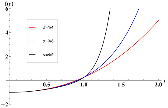
Figure 1.
The lapse function of black holes with in the scope of .
As a last comment, we must emphasize another peculiar behavior of the black holes in this particular range for : the geometry does not have a Cauchy (inner) horizon as usually seen in charged geometries, as the event horizon is the only one splitting the manifold in blocks.1
2.2. Theories in the Scope of
Here, s is also positive, and the range of allows for only (any) negative values of . According to (13), we can no longer extend the manifold beyond , as a curvature singularity is present in such a point. The asymptotic regions of f are given by
claiming the positive real solution of written in (12). In such a case, the signal of settles the number of event horizons of the solution: we may have two positive and real solutions for representing Cauchy () and event () horizons or no solution at all. Since, in our case, , the curvature scalars diverge at in the last case (no horizons), we have a naked curvature singularity. We can avoid that ill-defined spacetime (with a naked singularity) by limiting q.
Here, a threshold for the charge is achieved in the equation expressed as —representing solutions with a maximum charge of , i.e.,
which both the Cauchy and event horizons at the same point. As a consequence, whenever , we have a naked singularity, and for , the geometry possesses the usual two horizons. We can simplify the above equation by redefining , obtaining
or explicitly
In the present manuscript, for the above range, we consider the propagation of a scalar field only in well-defined spacetimes with two horizons, i.e., within , preventing the presence of a naked singularity. In Figure 2, we display three different panels representing the qualitative behaviors of .
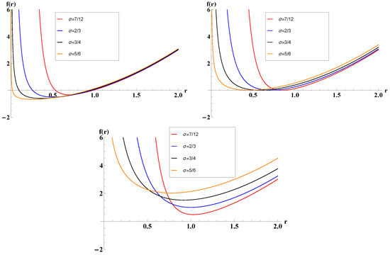
Figure 2.
The lapse-function profile of black holes with in the scope of with charges of (left), (middle) and (right).
2.3. Theories in the Scope of
In the last range for , we have s = −1 and . In this scope, we also cannot extend the Manifold beyond , as a curvature singularity is present at such a point. The asymptotic regions of f reads as follows:
Here, we have the same inflection point defined in (12), in which . After , f is a monotonically growing function defining exactly one solution to the equation expressed as , i.e., the event horizon. Again, we see no second horizon, despite the presence of electromagnetic charge, which makes the spacetime particularly peculiar. For such theories, we see no bounds in geometry constants and q (no naked singularity is present, regardless of their values). The lapse function in the last range is deployed in Figure 3.
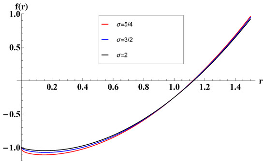
Figure 3.
The lapse function of black holes with in the scope of .
Once the causal structure with the possible limits on the geometry constants is settled, we are in a position to study the dynamical stability of the black holes in response to small field perturbations. In this article, we study a scalar field whose equation and methods are described in the next section.
3. Black-Hole Dynamics: Scalar Field Motion Equation
The starting point for studying scalar perturbations in black-holes background such as those described above is the Klein–Gordon relation:
which is obtained through the variation of the scalar-field matter action, . To develop (20), we choose the line element (5) in the null () and radial coordinates, bringing it to
Here, the Klein–Gordon equation in such a geometry is considerably simplified with a proper Ansatz for :
where k is the angular momentum of the field, ; and is the harmonic dependence on v, also known as the quasinormal frequency. The scalar equation can then be expressed as
V being the effective potential,
Equation (23) can be solved using several numerical methods available in previous literature [40,41,42,43,44,45,61,62,63,64,65,66]. We choose to work with the Frobenius method developed in [65]. To that end, Equation (23) must be written in coordinate form as follows ():
in which , and . To solve (25), we expand each function ( and u) around , i.e.,
and perform a similar expansion for , i.e.,
We balance the perturbation equation order by order matching each coefficient in the expansion. For the leading order, two values of are possible: and . The latter represents an outgoing wave from the event horizon (classically irrelevant), and is an ongoing front wave that we must consider for a physically relevant boundary condition. For a higher order, we have to satisfy the following recurrence relation:
Finally, at , we apply a condition according to which the field must maintain its physical relevance, that is, . This last relation can be numerically implemented by truncating the series in a specific number of terms (N), i.e.,
checking the convergence with a higher afterwards. The quasinormal spectrum is achievable trough the above method, the results of which we report in the next section.
4. Scalar-Field Quasinormal Modes
As a first step in our calculations with the scalar-field perturbations, we aim to reproduce the results presented, e.g., in [51] when . We accomplish that with a precision higher than . Particularly, in the case of presented in Table 1 and Table 2 we obtained, e.g., for as the highest deviation (cca ).

Table 1.
Quasinormal modes for theories with , high charge and zero angular momentum. The geometric parameters read .
Table 2.
Asymptotic quasinormal modes for theories with and zero angular momentum for the scalar field. The geometric parameters read .
The solutions for the linear theory ()—as mentioned in the Section 2—have been broadly studied in the literature since the original paper of 1992 and its companions [6,67,68]. Particularly, scalar perturbations were considered in [48,49] with their associated stability issues. For this reason, de do not treat those solutions in the present work.
After developing the Frobenius method numerically, we employ it with a series expansion of 45 terms, checking it afterwards with a 60-term series. The results exhibit very good convergence, with less than deviation. In Figure 4, we show the quasinormal modes for theories with considering multiple values of q.
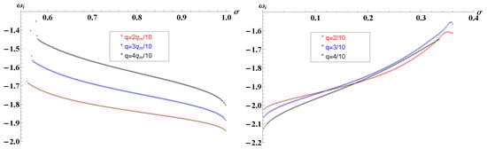
Figure 4.
The fundamental quasinormal modes of black holes in nonlinear electrodynamics. All solutions are purely imaginary, with no angular momentum (). The geometric parameters are .
As displayed in the figure, all the fundamental frequencies are purely imaginary in the case of a massless field with no angular momentum (). That is also the qualitative result found in other charged BTZ black holes, as shown in [48,51].
We emphasize two interesting features for the set of quasinormal modes we delivered in the panels. First of all, in theories with two horizons, we can see that an increase in the charge produces smaller values of . Such behavior is qualitatively the same as that found in [48,51], although in the linear theory, the variation is much more pronounced. Second, in such theories, the increment in diminishes such that values closer to cause vary very abruptly. (This also represents the limit of convergence of the presented method).
If we consider small values and one-horizon theories, the behavior is qualitatively the opposite as that displayed in the right panel of Figure 4. Smaller values of result in higher values, while an increase in the coefficient diminishes the corresponding fundamental quasinormal mode.
The peculiar structure of the modes demonstrated in both panels is an interesting novelty that locates as the special point of the series. Unfortunately, the available methods do not allow for the calculation of such theories due to the presence of in the lapse function (for this reason, any expansion near collapses the numerical solution).
We still pinpoint the departure value of quasinormal modes in both panels as for the presented series of theories, in accordance with special cases when (that would be a classical BTZ black hole without charge and with the cosmological constant rescaled) and when (also original black hole without charge, considering a rescale in the mass term).
In the range of , as we have no bound for the spacetime charge, we consider charges with higher values (and smaller , ), which is generally forbidden in charged black holes. The results are displayed in Table 1 and show that the oscillations are very sensitive to q presenting counter intuitive behavior: as we decrease —the area of the black hole (increasing q)—the absolute value of quasinormal modes increases (in contrast to the behavior reported in [65]).
It is interesting to notice the stating point of for as . In the case of , the frequency would be [47]. With our methods for , we obtained , and brings .
The last results we present for the scalar-field perturbations are those for black holes with one horizon and . In such a scope (), we investigate the response that different theories bring for scalar-field perturbations with fixed charges. The results are displayed in Figure 5.
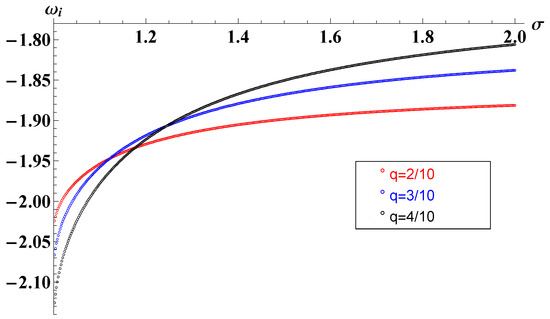
Figure 5.
The fundamental quasinormal modes of black holes in nonlinear electrodynamics. All the solutions are purely imaginary, with no angular momentum (). The geometric parameters are .
In the figure, we can observe an opposite relation between the increase in and the decrease in , asymptotically approaching a fixed value when . We calculate asymptotic quasinormal modes () with different charges in the limit of , and the results are listed in Table 2.
In the particular cases shown in Figure 5, we have , and for the asymptotic oscillations for charges of , and , respectively.
It is important to notice that all field dynamics studied in this section point in the direction of a stable spacetime for first-order scalar perturbationsas long as no frequencies were found with a positive coefficient () representing unstable evolutions. Although this fact does not constitute a mathematical proof of geometric stability in response to first-order perturbations, it strongly suggests that the black holes of such theories react to a massless and changeless scalar field with a tower of quasinormal oscillations decaying in time, thereby keeping the event horizon of the black hole and the fabric of spacetime intact.
5. Final Remarks
In this work, we studied black holes in 2 + 1 nonlinear electrodynamic theories.
The geometry of different line elements representing possible solutions was studied, particularly in relation to the presence of horizons. We found a rich causal structure depending on the considered coefficient. Interestingly enough, the spacetime is regular at only for small values.
In the case of , we found that black holes are regular at with one event horizon in all possible solutions with charge, mass and cosmological constant. That is clearly not the case of the linear theories either in 2 + 1 or higher dimensional spacetimes.
Intermediate values of in the scope of bring solutions with two or no horizons, depending on the values of the geometric constants. As common to other charged spacetimes, in such cases, we have a maximum value of charge, calculated using Equation (18), depending on and , as a naked curvature singularity is present at .
For high values of , we also have one horizon present for every charge, mass and cosmological constant. The behavior is essentially distinct from that presented for intermediate values (and linear theories) of the change of s in (9). In such cases, we have a curvature singularity at hidden by the event horizon.
We also studied the propagation of a scalar field delivered via matter action in all three types of theories. Our results strongly suggest the spacetimes to be stable to first-order perturbations, with the scalar-field evolution being given in terms of the typical quasinormal evolution. The quasinormal spectra of the different theories were calculated in Section 4. They show an intriguing peculiarity of a diminishing as approaches . In the cases of an asymptotic , , and for high charges, increases unboundedly with q. Interestingly enough, that behavior points in the opposite direction of the interpretation of as being proportional to the Hawking temperature of the hole [65], therefore not representing the relaxation time of the lower dimensional conformal field theory: in such cases, [54], decreasing with the increment of q. Such an interpretation is also lost in the near-extremal cases of the linear theory of a charged BTZ black hole (see, e.g., [48]), although for intermediate and small values, it endures.
Further lines of investigation include the inspection of super-radiant phenomena that may be associated with charged scalar propagation and the perturbations delivered by fields of different spins. Also interesting is the examination of rotating black holes with non-linear electrodynamic terms, as well as those with acceleration [31], as brought up by one of our anonymous referees.
Funding
This work was partially supported by CNPq (Conselho Nacional de Desenvolvimento Científico-Brazil) under Grant No. 405749/2023-6.
Data Availability Statement
The original contributions presented in this study are included in the article. Further inquiries can be directed to the corresponding author.
Acknowledgments
The author would like to thank J.S.E. Portela and J. de Oliveira for fruitful discussions.
Conflicts of Interest
The author declares no conflicts of interest.
Note
| 1 | It is still worth mentioning the singularity of the chargeless BTZ geometry without rotation as being associated with an angular deficit in if the line element is considered isometric to the pure AdS geometry. |
References
- Deser, S.; Jackiw, R. Three-Dimensional Cosmological Gravity: Dynamics of Constant Curvature. Ann. Phys. 1984, 153, 405–416. [Google Scholar] [CrossRef]
- Carlip, S. Classical general relativity in 2 + 1 dimensions. In Quantum Gravity in 2 + 1 Dimensions; Cambridge Monographs on Mathematical Physics, Cambridge University Press: Cambridge, UK, 1998. [Google Scholar]
- García-Díaz, A.A. Dilaton–Inflaton Friedmann–Robertson–Walker Cosmologies. In Exact Solutions in Three-Dimensional Gravity; Cambridge Monographs on Mathematical Physics, Cambridge University Press: Cambridge, UK, 2017. [Google Scholar]
- Arenas-Henriquez, G.; Gregory, R.; Scoins, A. On acceleration in three dimensions. J. High Energy Phys. 2022, 2022, 63. [Google Scholar] [CrossRef]
- Arenas-Henriquez, G.; Cisterna, A.; Diaz, F.; Gregory, R. Accelerating Black Holes in 2+1 dimensions: Holography revisited. arXiv 2023, arXiv:2308.00613. [Google Scholar] [CrossRef]
- Banados, M.; Teitelboim, C.; Zanelli, J. The Black hole in three-dimensional space-time. Phys. Rev. Lett. 1992, 69, 1849–1851. [Google Scholar] [CrossRef]
- Jackiw, R. Lower Dimensional Gravity. Nucl. Phys. B 1985, 252, 343–356. [Google Scholar] [CrossRef]
- Mann, R.B. Lower dimensional black holes. Gen. Rel. Grav. 1992, 24, 433–449. [Google Scholar] [CrossRef]
- de Oliveira, J.; Fontana, R.D.B. Three-dimensional black holes with quintessence. Phys. Rev. D 2018, 98, 044005. [Google Scholar] [CrossRef]
- Bueno, P.; Andino, O.L.; Moreno, J.; van der Velde, G. On regular charged black holes in three dimensions. arXiv 2025, arXiv:2503.02930. [Google Scholar]
- Kiselev, V.V. Quintessence and black holes. Class. Quantum Gravity 2003, 20, 1187. [Google Scholar] [CrossRef]
- Holst, S.; Matschull, H.J. The Anti-de Sitter Gott universe: A Rotating BTZ wormhole. Class. Quant. Grav. 1999, 16, 3095–3131. [Google Scholar] [CrossRef]
- Cataldo, M.; Cruz, N.; del Campo, S.; Garcia, A. (2 + 1)-dimensional black hole with Coulomb-like field. Phys. Lett. B 2000, 484, 154. [Google Scholar] [CrossRef]
- Emparan, R.; Frassino, A.M.; Way, B. Quantum BTZ black hole. JHEP 2020, 11, 137. [Google Scholar] [CrossRef]
- Koch, B.; Reyes, I.A.; Rincón, A. A scale dependent black hole in three-dimensional space–time. Class. Quant. Grav. 2016, 33, 225010. [Google Scholar] [CrossRef]
- Contreras, E.; Rincón, A.; Bargueño, P. A general interior anisotropic solution for a BTZ vacuum in the context of the Minimal Geometric Deformation decoupling approach. Eur. Phys. J. C 2019, 79, 216. [Google Scholar] [CrossRef]
- Younesizadeh, Y.; Ahmed, A.H.; Ahmad, A.A.; Younesizadeh, F.; Ebrahimkhas, M. What happens for the BTZ black hole solution in dilaton f(R)-gravity? Int. J. Mod. Phys. D 2021, 30, 2150028. [Google Scholar] [CrossRef]
- Ahmed, F.; Bouzenada, A. Stationary BTZ space-time in Ricci-inverse and f(R) gravity theories. Eur. Phys. J. C 2024, 84, 1271. [Google Scholar] [CrossRef]
- Nashed, G.; Sheykhi, A. New black hole solutions in three-dimensional f(R) gravity. Phys. Dark Universe 2023, 40, 101174. [Google Scholar] [CrossRef]
- Chen, W.X.; Zheng, Y.G. Thermodynamic geometric analysis of BTZ black hole under f(R) gravity. arXiv 2022, arXiv:2112.15032. [Google Scholar]
- Fernando, S. Quasinormal modes of charged scalars around dilaton black holes in 2+1 dimensions: Exact frequencies. Phys. Rev. D 2008, 77, 124005. [Google Scholar] [CrossRef]
- Fernando, S. Quasinormal Modes of Charged Dilaton Black Holes in 2 + 1 Dimensions. Gen. Relativ. Gravit. 2004, 36, 71–82. [Google Scholar] [CrossRef]
- González, P.; Papantonopoulos, E.; Saavedra, J. Chern-Simons black holes: Scalar perturbations, mass and area spectrum and greybody factors. J. High Energy Phys. 2010, 2010, 50. [Google Scholar] [CrossRef]
- Övgün, A.; Jusufi, K. Quasinormal modes and greybody factors of f(R) gravity minimally coupled to a cloud of strings in 2 + 1 dimensions. Ann. Phys. 2018, 395, 138–151. [Google Scholar] [CrossRef]
- Birmingham, D.; Sachs, I.; Sen, S. Exact results for the BTZ black hole. Int. J. Mod. Phys. D 2001, 10, 833–858. [Google Scholar] [CrossRef]
- Birmingham, D.; Sachs, I.; Solodukhin, S.N. Conformal Field Theory Interpretation of Black Hole Quasinormal Modes. Phys. Rev. Lett. 2002, 88, 151301. [Google Scholar] [CrossRef]
- Lee, H.W.; Myung, Y.S. Greybody factor for the BTZ black hole and a 5-D black hole. Phys. Rev. D 1998, 58, 104013. [Google Scholar] [CrossRef]
- Dasgupta, A. Emission of fermions from BTZ black holes. Phys. Lett. B 1999, 445, 279–286. [Google Scholar] [CrossRef]
- Rincón, A.; Villanueva, J.R. The Sagnac effect on a scale-dependent rotating BTZ black hole background. Class. Quant. Grav. 2020, 37, 175003. [Google Scholar] [CrossRef]
- Cuadros-Melgar, B.; Fontana, R.D.B.; de Oliveira, J. Gauss-Bonnet black holes in (2+1) dimensions: Perturbative aspects and entropy features. Phys. Rev. D 2022, 106, 124007. [Google Scholar] [CrossRef]
- Fontana, R.D.B.; Rincon, A. Accelerated black holes in (2 + 1) dimensions: Quasinormal modes and stability. Eur. Phys. J. C 2025, 85, 179. [Google Scholar] [CrossRef]
- Regge, T.; Wheeler, J.A. Stability of a Schwarzschild singularity. Phys. Rev. 1957, 108, 1063–1069. [Google Scholar] [CrossRef]
- Addesso, P.; Adhikari, R.; Adya, V.; Affeldt, C.; Agathos, M.; Agatsuma, K.; Aggarwal, N.; Aguiar, O.; Aiello, L.; Ain, A.; et al. Observation of Gravitational Waves from a Binary Black Hole Merger. Phys. Rev. Lett. 2016, 116, 061102. [Google Scholar] [CrossRef]
- Addesso, P.; Adhikari1, R.; Adya, V.; Affeldt, C.; Agathos, M.; Agatsuma, K.; Aggarwal, N.; Aguiar, O.; Aiello, L.; Ain, A.; et al. GW151226: Observation of Gravitational Waves from a 22-Solar-Mass Binary Black Hole Coalescence. Phys. Rev. Lett. 2016, 116, 241103. [Google Scholar] [CrossRef]
- Adhikari, R.; Adya, V.; Affeldt, C.; Afrough, M.; Agarwal, B.; Agathos, M.; Agatsuma, K.; Aggarwal, N.; Aguiar, O.; Aiello, L.; et al. GW170104: Observation of a 50-Solar-Mass Binary Black Hole Coalescence at Redshift 0.2. Phys. Rev. Lett. 2017, 118, 221101, Erratum in Phys. Rev. Lett. 2018, 121, 129901. [Google Scholar] [CrossRef]
- Zerilli, F.J. Gravitational field of a particle falling in a schwarzschild geometry analyzed in tensor harmonics. Phys. Rev. D 1970, 2, 2141–2160. [Google Scholar] [CrossRef]
- Zerilli, F.J. Effective potential for even parity Regge-Wheeler gravitational perturbation equations. Phys. Rev. Lett. 1970, 24, 737–738. [Google Scholar] [CrossRef]
- Teukolsky, S.A. Rotating black holes—Separable wave equations for gravitational and electromagnetic perturbations. Phys. Rev. Lett. 1972, 29, 1114–1118. [Google Scholar] [CrossRef]
- Teukolsky, S.A.; Press, W.H. Perturbations of a rotating black hole. III - Interaction of the hole with gravitational and electromagnetic radiation. Astrophys. J. 1974, 193, 443–461. [Google Scholar] [CrossRef]
- Leaver, E.W. Spectral decomposition of the perturbation response of the Schwarzschild geometry. Phys. Rev. D 1986, 34, 384–408. [Google Scholar] [CrossRef]
- Leaver, E.W. Quasinormal modes of Reissner-Nordström black holes. Phys. Rev. D 1990, 41, 2986–2997. [Google Scholar] [CrossRef]
- Schutz, B.F.; Will, C.M. Black hole normal modes—A semianalytic approach. Astrophysic. J. 1985, 291, L33–L36. [Google Scholar] [CrossRef]
- Iyer, S.; Will, C.M. Black Hole Normal Modes: A WKB Approach. 1. Foundations and Application of a Higher Order WKB Analysis of Potential Barrier Scattering. Phys. Rev. 1987, D35, 3621. [Google Scholar] [CrossRef] [PubMed]
- Iyer, S. Black-hole normal modes: A WKB approach. II. Schwarzschild black holes. Phys. Rev. D 1987, 35, 3632–3636. [Google Scholar] [CrossRef] [PubMed]
- Kokkotas, K.D.; Schutz, B.F. Black Hole Normal Modes: A WKB Approach. 3. The Reissner-Nordstrom Black Hole. Phys. Rev. 1988, D37, 3378–3387. [Google Scholar] [CrossRef] [PubMed]
- Cardoso, V.; Lemos, J.P.S. Scalar, electromagnetic, and Weyl perturbations of BTZ black holes: Quasinormal modes. Phys. Rev. D 2001, 63, 124015. [Google Scholar] [CrossRef]
- Birmingham, D. Choptuik scaling and quasinormal modes in the anti–de Sitter space/conformal-field theory correspondence. Phys. Rev. D 2001, 64, 064024. [Google Scholar] [CrossRef]
- Fontana, R.D.B. Quasinormal modes of charged BTZ black holes. Class. Quantum Gravity 2024, 41, 145010. [Google Scholar] [CrossRef]
- Fontana, R.D.B. Scalar field instabilities in charged BTZ black holes. Phys. Rev. D 2024, 109, 044039. [Google Scholar] [CrossRef]
- Konewko, S.; Winstanley, E. Charge superradiance on charged BTZ black holes. Eur. Phys. J. C 2024, 84, 594. [Google Scholar] [CrossRef]
- Aragón, A.; González, P.A.; Saavedra, J.; Vásquez, Y. Scalar quasinormal modes for 2 + 1-dimensional Coulomb-like AdS black holes from nonlinear electrodynamics. Gen. Relativ. Gravit. 2021, 53, 91. [Google Scholar] [CrossRef]
- González, P.; Rincón, Á.; Saavedra, J.; Vásquez, Y. Superradiant instability and charged scalar quasinormal modes for (2 + 1)-dimensional Coulomb-like AdS black holes from nonlinear electrodynamics. Phys. Rev. D 2021, 104. [Google Scholar] [CrossRef]
- Hendi, S.H. Charged BTZ-like black holes in higher dimensions. Eur. Phys. J. C 2011, 71, 1551. [Google Scholar] [CrossRef]
- Hendi, S.H.; Eslam Panah, B.; Saffari, R. Exact solutions of three-dimensional black holes: Einstein gravity versus F(R) gravity. Int. J. Mod. Phys. D 2014, 23, 1450088. [Google Scholar] [CrossRef]
- Younesizadeh, Y.; Ahmad, A.A.; Ahmed, A.H.; Younesizadeh, F.; Ebrahimkhas, M. A new black hole solution in dilaton gravity inspired by power-law electrodynamics. Int. J. Mod. Phys. A 2019, 34, 1950239. [Google Scholar] [CrossRef]
- Valtancoli, P. Scalar field conformally coupled to a charged BTZ black hole. Ann. Phys. 2016, 369, 161–167. [Google Scholar] [CrossRef]
- Panotopoulos, G.; Rincón, A. Quasinormal modes of black holes in Einstein-power-Maxwell theory. Int. J. Mod. Phys. D 2018, 27, 1850034. [Google Scholar] [CrossRef]
- Soroushfar, S.; Saffari, R.; Jafari, A. Study of geodesic motion in a (2+1)-dimensional charged BTZ black hole. Phys. Rev. D 2016, 93, 104037. [Google Scholar] [CrossRef]
- Nascimento, F.F.d.; Bezerra, V.B.; Toledo, J.d.M. Black Holes with a Cloud of Strings and Quintessence in a Non-Linear Electrodynamics Scenario. Universe 2024, 10, 430. [Google Scholar] [CrossRef]
- Kruglov, S.I. Einstein-AdS Gravity Coupled to Nonlinear Electrodynamics, Magnetic Black Holes, Thermodynamics in an Extended Phase Space and Joule–Thomson Expansion. Universe 2023, 9, 456. [Google Scholar] [CrossRef]
- Seidel, E.; Iyer, S. Black hole normal modes: A WKB approach. 4. Kerr black holes. Phys. Rev. 1990, D41, 374–382. [Google Scholar] [CrossRef]
- Konoplya, R.A. Quasinormal behavior of the d-dimensional Schwarzschild black hole and higher order WKB approach. Phys. Rev. 2003, D68, 024018. [Google Scholar] [CrossRef]
- Matyjasek, J.; Opala, M. Quasinormal modes of black holes: The improved semianalytic approach. Phys. Rev. D 2017, 96, 024011. [Google Scholar] [CrossRef]
- Gundlach, C.; Price, R.H.; Pullin, J. Late-time behavior of stellar collapse and explosions. I. Linearized perturbations. Phys. Rev. D 1994, 49, 883–889. [Google Scholar] [CrossRef]
- Horowitz, G.T.; Hubeny, V.E. Quasinormal modes of AdS black holes and the approach to thermal equilibrium. Phys. Rev. D 2000, 62, 024027. [Google Scholar] [CrossRef]
- Jansen, A. Overdamped modes in Schwarzschild-de Sitter and a Mathematica package for the numerical computation of quasinormal modes. Eur. Phys. J. Plus 2017, 132, 546. [Google Scholar] [CrossRef]
- Carlip, S. The (2 + 1)-dimensional black hole. Class. Quantum Gravity 1995, 12, 2853–2879. [Google Scholar] [CrossRef]
- Martínez, C.; Teitelboim, C.; Zanelli, J. Charged rotating black hole in three spacetime dimensions. Phys. Rev. D 2000, 61. [Google Scholar] [CrossRef]
Disclaimer/Publisher’s Note: The statements, opinions and data contained in all publications are solely those of the individual author(s) and contributor(s) and not of MDPI and/or the editor(s). MDPI and/or the editor(s) disclaim responsibility for any injury to people or property resulting from any ideas, methods, instructions or products referred to in the content. |
© 2025 by the author. Licensee MDPI, Basel, Switzerland. This article is an open access article distributed under the terms and conditions of the Creative Commons Attribution (CC BY) license (https://creativecommons.org/licenses/by/4.0/).