Article

A Novel Logarithmic Approach to General Relativistic Hydrodynamics in Dynamical Spacetimes

1
Dipartimento di Fisica, Università della Calabria, Via Pietro Bucci, Arcavacata, 87036 Cosenza, Italy
2
Dipartimento di Fisica e Astronomia, Università Degli Studi di Firenze e INFN-Sezione di Firenze, Via G. Sansone 1, Sesto Fiorentino, 50019 Firenze, Italy
3
Istituto Nazionale di Astrofisica (INAF)-Osservatorio Astrofisico di Arcetri, Largo E. Fermi 5, 50125 Firenze, Italy
*
Author to whom correspondence should be addressed.
Universe 2025, 11(6), 194; https://doi.org/10.3390/universe11060194
Submission received: 10 May 2025 / Revised: 15 June 2025 / Accepted: 16 June 2025 / Published: 18 June 2025

Abstract

We introduce a novel logarithmic approach within the Baumgarte–Shapiro–Shibata–Nakamura (BSSN) formalism for self-consistently solving the equations of general relativistic hydrodynamics (GRHD) in evolving curved spacetimes. This method employs a “3 + 1” decomposition of spacetime, complemented by the “1 + log” slicing condition and Gamma-driver shift conditions, which have been shown to improve numerical stability in spacetime evolution. A key innovation of our work is the logarithmic transformation applied to critical variables such as rest-mass density, energy density, and pressure, thus preserving physical positivity and mitigating numerical issues associated with extreme variations. Our formulation is fully compatible with advanced numerical techniques, including spectral methods and Fourier-based algorithms, and it is particularly suited for simulating highly nonlinear regimes in which gravitational fields play a significant role. This approach aims to provide a solid foundation for future numerical implementations and investigations of relativistic hydrodynamics, offering promising new perspectives for modeling complex astrophysical phenomena in strong gravitational fields, including matter evolution around compact objects like neutron stars and black holes, turbulent flows in the early universe, and the nonlinear evolution of cosmic structures.

1. Introduction

Multi-messenger astrophysics has emerged as one of the most active and rapidly developing areas in modern astrophysics. In this context, the numerical investigation of matter dynamics around compact objects, such as black holes and neutron stars, where spacetime is highly curved, has become increasingly central. Understanding these systems is crucial not only for modeling the complex behavior of accretion disks, jets, and the resulting radiation emitted from extreme merger events but also for exploring a broader class of astrophysical and cosmological scenarios, including the dynamics of the early universe, structure formation, and the evolution of turbulent relativistic fluids in strong gravitational fields [1,2,3,4]. A fundamental requirement for these studies is a robust formulation of relativistic hydrodynamics (RHD) in curved spacetime, where consistent coupling with the Einstein field equations is essential to accurately describe the interplay between fluid dynamics and spacetime curvature. Although general relativistic magnetohydrodynamics (GRMHD) provides a comprehensive framework by incorporating magnetic fields, general relativistic hydrodynamics (GRHD) remains indispensable for investigating purely hydrodynamic processes in regimes where magnetic effects, while relevant in many astrophysical environments [5], are subdominant. This is particularly relevant in several astrophysical contexts, such as the evolution of relativistic outflows, accretion dynamics, or matter interactions in merger remnants [6,7,8]. Moreover, GRHD plays a fundamental role in early-universe studies, where, despite the potential relevance of primordial magnetic fields [9,10], a hydrodynamic treatment often represents the leading-order approximation. In such scenarios, the analysis of RHD in an expanding universe is critical for understanding large-scale structure formation and the evolution of turbulent cosmic flows.
Significant advances in numerical methods for solving the GRHD equations have emerged in recent decades. Wilson’s pioneering work [11] laid the foundations for RHD simulations, which were subsequently refined to enhance resolution and stability [12,13]. The “3 + 1” decomposition of spacetime, initially introduced by Arnowitt, Deser, and Misner (ADM) [14] and further developed through the Bumgarte–Shapiro–Shibata–Nakamura (BSSN) formalism [15,16] has been fundamental in stabilizing simulations of highly dynamic spacetimes, including binary mergers and stellar collapses [17,18,19]. While high-precision simulations in cosmology have traditionally relied on perturbative techniques or Newtonian gravity approximations [20,21], as well as post-Newtonian approaches [22,23,24], recent measurements from missions such as Planck [25], the Dark Energy Survey [26], and forthcoming data from Euclid [27] are pushing observational precision to the sub-percent levels, highlighting the need for a more reliable and accurate numerical techniques. In addition to cosmological applications, fully relativistic simulations have become essential to study magnetized plasma dynamics around compact objects, where strong gravitational fields and relativistic effects play a central role in processes such as jet formation, accretion, and magnetic reconnection [28,29,30].
Spectral methods, renowned for their high precision, are able to capture intricate system details, yet balancing accuracy and stability requires a careful integration of filtering techniques and controlled dissipation mechanisms to mitigate numerical instabilities. In this work, we introduce a logarithmic formulation of the GRHD equations within the “3 + 1” framework, designed to enhance numerical stability under extreme conditions. Beyond its immediate application to GRHD, this formalism may be promising for investigating the nonlinear evolution of compact objects and the surrounding matter, as well as cosmic structures, where standard perturbative techniques or Newtonian approximations may prove inadequate. In scenarios where structure formation leads to large mass–energy contrasts, steep gradients, and shocks, the logarithmic formulation may provide a natural framework for handling the resulting extreme dynamical ranges. Similarly, in turbulent regimes coupled to the Einstein equations, localized amplification processes can lead to density contrasts spanning several orders of magnitude. In these settings, the combination of a logarithmic formulation with Fourier-based spectral methods may prove particularly effective in handling the evolution of large variations in physical quantities.
Although spectral schemes are known for their excellent precision, they are highly sensitive to sharp features in the solution. The logarithmic formulation is designed to mitigate and potentially allow a better resolution of moderately steep gradients and discontinuities. Consequently, this approach may retain more physical information than widely used shock-capturing techniques, such as high-resolution shock-capturing (HRSC) methods [31,32], which, despite their robustness, tend to introduce significant numerical dissipation in highly dynamical regimes.
The paper is structured as follows: Section 2 introduces the “3 + 1” logarithmic GRHD formulation, detailing the transformation of conserved variables and the corresponding evolution equations; Section 3 presents a preliminary set of applications of the logarithmic formulation within a flat spacetime framework; Section 4 provides the full set of GRHD equations to be evolved and discusses potential astrophysical applications; Section 5 concludes with final remarks. Throughout the present work, we adopt geometrized units ( c = G = 1 ), with Greek indices ( μ , ν , ) representing spacetime coordinates and Latin indices ( i , j , ) representing spatial coordinates.

2. The “3 + 1” Logarithmic Approach to GRHD

In this section, we present a logarithmic formulation of the GRHD equations within a “3 + 1” framework, utilizing the BSSN formalism for spacetime evolution [15,17]. This approach is based on the Hamiltonian formulation of general relativity, where spacetime is foliated into space-like hypersurfaces Σ . We adopt the “3 + 1” decomposition of the Einstein field equations, as implemented in the BSSN approach, following the procedure outlined by Campanelli et al. [19], which has been successfully applied in previous studies (e.g., Imbrogno et al. [33]). The complete set of equations, including the matter terms, is given by
( t β k k ) γ ˜ i j = 2 α A ˜ i j + γ ˜ i k j β k + γ ˜ k j i β k 2 3 γ ˜ i j k β k ,
( t β i i ) χ = 2 3 χ α K i β i
( t β k k ) A ˜ i j = α K A ˜ i j 2 A ˜ i k γ ˜ m k A ˜ m j + χ i j α + α R i j TF + A ˜ i k j β k + A ˜ k j i β k 2 3 A ˜ i j k β k + 4 π α γ ˜ i j ( S E ) 2 γ ˜ i l γ ˜ j m S l m χ TF ,
( t β i i ) K = 2 α + α A ˜ l m A ˜ l m + 1 3 K 2 + 4 π α ( E + S ) ,
( t β j j ) Γ ˜ i = γ ˜ l m l m β i + 1 3 γ ˜ i l l m β m Γ ˜ k k β i + 2 3 Γ ˜ i k β k 2 A ˜ i k k α + α 2 Γ ˜ l m i A ˜ l m 3 χ A ˜ i k k χ 4 3 γ ˜ i k k K 16 π S i ,
( t β i i ) α = α 2 f ( α ) K ,
t β i = B i ,
t B i = 3 4 t Γ ˜ i η B i .
The above equations arise from a conformal rescaling of the three-metric γ ˜ i j = χ γ i j , where χ = γ 1 / 3 is the conformal factor, with  γ being the determinant of the spatial three-metric γ i j [19]. The extrinsic curvature K i j is decomposed into its trace K and trace-free part A i j , given by A i j = χ 1 A ˜ i j , where A ˜ i j = χ ( K i j 1 3 γ i j K ) . This formulation introduces the contracted Christoffel symbols, Γ ˜ i = γ ˜ j k Γ ˜ j k i , evolving according to Equation (5). The lapse function is denoted by α , β i represents the shift vector, i is the covariant derivative in physical space, 2 = γ i j i j is the Laplacian on a spatial hypersurface,  R i j is the purely spatial Ricci tensor, and the superscript “TF” stands for the trace-free part of a tensor. Equations (6)–(8) govern the evolution of the lapse and shift vector following the Bona-Massó family of slicing conditions [16,34,35]. In the former, f ( α ) is a freely specifiable function that determines the slicing condition and can be selected to achieve different gauge properties for the lapse, with the widely used ”1 + log” slicing corresponding to the choice f ( α ) = 2 / α ; in the latter, B i is an auxiliary variable introduced to rewrite the shift condition in first-order form and  η is a damping parameter that promotes numerical stability [36]. These choices define the “Gamma-driver” shift condition, which is particularly robust for puncture initial data, effectively controlling slice stretching and rotational shear in singular or near-singular spacetimes [37]. Finally, we adopt f ( α ) = 1 / α , corresponding to the “ 1 + log ” slicing condition, widely used in compact object simulations. In the presence of matter, additional terms appear, namely E, S i , and  S i j , representing the total mass–energy density, momentum density, and stress tensor, respectively, as measured by a normal observer (Eulerian observer). Additionally, S = χ 1 γ ˜ i j S i j denotes the trace of the stress tensor.
As discussed in [18,38,39,40,41], all “3 + 1” fields must satisfy the Hamiltonian and momentum constraints, expressed in terms of the conformal transformation as
H = R A ˜ l m A ˜ l m + 2 3 K 2 16 π E = 0 ,
M i = k A ˜ i k + Γ ˜ l m i A ˜ l m 3 2 χ A ˜ i k k χ 2 3 γ ˜ i k k K 8 π χ S i = 0 .
In numerical simulations, we enforce T r { A ˜ i j } = 0 and impose γ ˜ = 1 to maintain a unit determinant for the conformal three-metric. For numerical stability, Γ ˜ i is replaced by j γ ˜ i j in all evolution equations where it is not explicitly differentiated [19].
In RHD, the conservation of mass, momentum, and energy is governed by the continuity equation and the stress–energy tensor, T μ ν = ( ρ + P ) u μ u ν + P g μ ν , where ρ is the total mass–energy density as measured in the fluid’s co-moving frame (Lagrangian observer), P is the pressure, u μ is the four-velocity term, and  g μ ν is the spacetime metric. The mass–energy density is typically split as ρ = ρ 0 ( 1 + ζ ) , where ζ is the specific internal energy. The evolution of the fluid is described by two conservation laws, one for rest mass and three for energy, momentum, and an equation of state (EoS) for the pressure:
μ ( ρ 0 u μ ) = 0 ,
μ T μ ν = 0 ,
P = P ( ρ 0 , h ) ,
where μ is the covariant derivative with respect to the four-metric g μ ν , ρ 0 is the rest-mass energy density (measured by an Eulerian observer), and h is the specific enthalpy. Employing the “3 + 1” formalism, the stress–energy tensor is decomposed using the contravariant spatial metric γ i j and the unit normal vector n μ to the hypersurface Σ . The resulting components are expressed as
E = ρ 0 h W 2 P = τ + D ,
S i = ρ 0 h W 2 v i ,
S i j = ρ 0 h W 2 v i v j + γ i j P = S i v j + γ i j P ,
where D is the rest-mass energy density and  τ denotes the difference between the total energy density and the rest-mass energy density. The velocity of the fluid v i is related to the four-velocity term by v i = u i / W , v i = u i / W + β i / α , where W = α u 0 = ( 1 v i v i ) 1 / 2 is the Lorentz factor.
The state of the fluid is characterized by the primitive variables ( ρ 0 , v i , P), from which the conserved variables are derived as D = ρ 0 W , S i = Equation (15), and  τ = ρ 0 h W 2 P D , where the specific enthalpy h is determined from the equation of state (EoS). In this study, we assume a barotropic ideal-fluid EoS characterized by a constant adiabatic index Γ , which corresponds to either of the following:
h = 1 + Γ Γ 1 P ρ 0 , h = 1 + Γ Γ 1 κ ρ 0 Γ 1 ,
where κ is the pseudo-entropy and Γ = 4 / 3 is the adiabatic index, assumed constant throughout the evolution. These conserved variables satisfy the relevant conservation laws, enabling their direct evolution in numerical simulations. The relation between conserved and primitive variables is nontrivial, and inversion is usually performed using an iterative root-finding algorithm, such as the Newton–Raphson method. To improve convergence, the method proposed by Mignone et al. [42] is adopted, which significantly reduces the number of iterations and ensures numerical robustness, avoiding the need to store primitive variables from previous time steps, as shown by Baiotti et al. [43], Galeazzi et al. [44].
The fluid evolution in curved spacetime is governed by the conservation laws of mass, momentum, and energy. These laws, when expressed within the “3 + 1” GRHD framework, are written as follows (see, e.g., Alcubierre [37] ([Chapter 7.4]) and Baiotti et al. [45]):
( t β i i ) D = α K D i α D v i ,
( t β j j ) S i = τ + D i α + α K S i S j j β i j α S i v j + γ i j P ,
( t β i i ) τ = τ + P + D α v j v l K j l v j j α + α K τ + P i α v i τ + P
We now manipulate the above equations as follows: a logarithmic transformation is applied specifically to the rest-mass density D, the energy density τ , and the pressure P, as these scalar quantities are particularly prone to discontinuities and are inherently well-suited for logarithmic representation, unlike quantities such as the three-velocity v i , which can assume both positive and negative values. In this way, the evolution equations in Equations (18)–(20) become less sensitive to large variations in these quantities, thereby enhancing numerical stability, particularly when using pseudo-spectral methods.
For the mass conservation equation, we introduce the logarithmic rest-mass density δ , defined as
δ = ln D D 0 ,
where D 0 denotes a reference value of D used to normalize Equation (18), leading to the following evolution equation for δ :
( t β i i ) δ = α K α v i i δ i α v i ,
where all relevant variables have been previously introduced.
For the momentum density equation, we define the new primitive variable σ i = h u i = h W v i , where v i represents the three-velocity term of the fluid. This choice allows us to express the momentum density as
S i = ρ 0 h W 2 v i = ( ρ 0 W ) ( h W v i ) = D σ i = D 0 e δ σ i ,
where δ is the logarithmic scaling factor introduced in Equation (21). To maintain dimensional consistency and ensure the uniform treatment of hydrodynamic variables, we introduce an additional logarithmic variable for the pressure, defined as π = ln P / D 0 1 This definition enables us to express all thermodynamic quantities in a dimensionless form, which is essential for preserving the validity of the equations under unit transformations. Moreover, pressure and energy density, whose logarithmic representation will be introduced shortly, often span comparable dynamical ranges, particularly in high-enthalpy relativistic flows such as those found in pulsar wind nebulae or gamma-ray bursts, making it both natural and consistent to treat them on equal footing. Starting from Equation (19), the evolution equation for σ i becomes
( t β j j ) σ i = 1 + e ε δ + e π δ γ i j j α e π δ α γ i j j π σ j j β i α v j j σ i .
The above equation incorporates the pressure gradient and accounts for spacetime curvature effects, represented by the extrinsic curvature as well as the lapse and shift functions.
Finally, for the energy density τ , we introduce the logarithmic variable ε , defined as
ε = ln τ D 0 ,
so that the evolution Equation (20), in its logarithmic form, reads as
( t β i i ) ε = α v i i ε + α v i v j K i j v j j α + α K i α v i 1 + e π ε + α v i v j K i j e δ ε v j j α e δ ε e π ε α v i i π .
The above relation governs the evolution of the energy density, ensuring that the effects of both the fluid’s motion and spacetime curvature are properly accounted for.
To validate this approach, we plan to integrate an appropriate module into well-established SFINGE code [46], which utilizes FFT and a stability check at each time step to ensure compliance with the Courant–Friedrichs–Lewy condition. It also implements periodic boundary conditions on a periodic mesh and includes a routine based on the Implicit Hyperviscous Boundary (IHB) method to reduce artifacts from domain periodicity. This is achieved by introducing a hyperviscous term into the evolution equations, which are then solved using an implicit Crank–Nicolson scheme [47]. This methodology is expected to offer advantages for simulating accreting matter around compact objects, as well as for cosmological problems involving periodic contractions, such as the formation of large-scale structures or the behavior of perturbations in the early universe.

3. Preliminary Numerical Applications

As a preliminary validation of the logarithmic approach, we performed some tests within a flat spacetime framework. Adopting a flat Minkowskian metric allows for a controlled investigation of two fundamental scenarios, namely the nonlinear propagation of sound waves and the subsequent nonlinear development of the Kelvin–Helmholtz instability (KHI). By eliminating the complications introduced by spacetime curvature, this setup allows for a more focused assessment of the numerical methods and their stability. These tests, albeit basic, serve to validate the robustness of the logarithmic formulation and provide further insights into the dynamics of relativistic fluids across a range of astrophysical contexts.

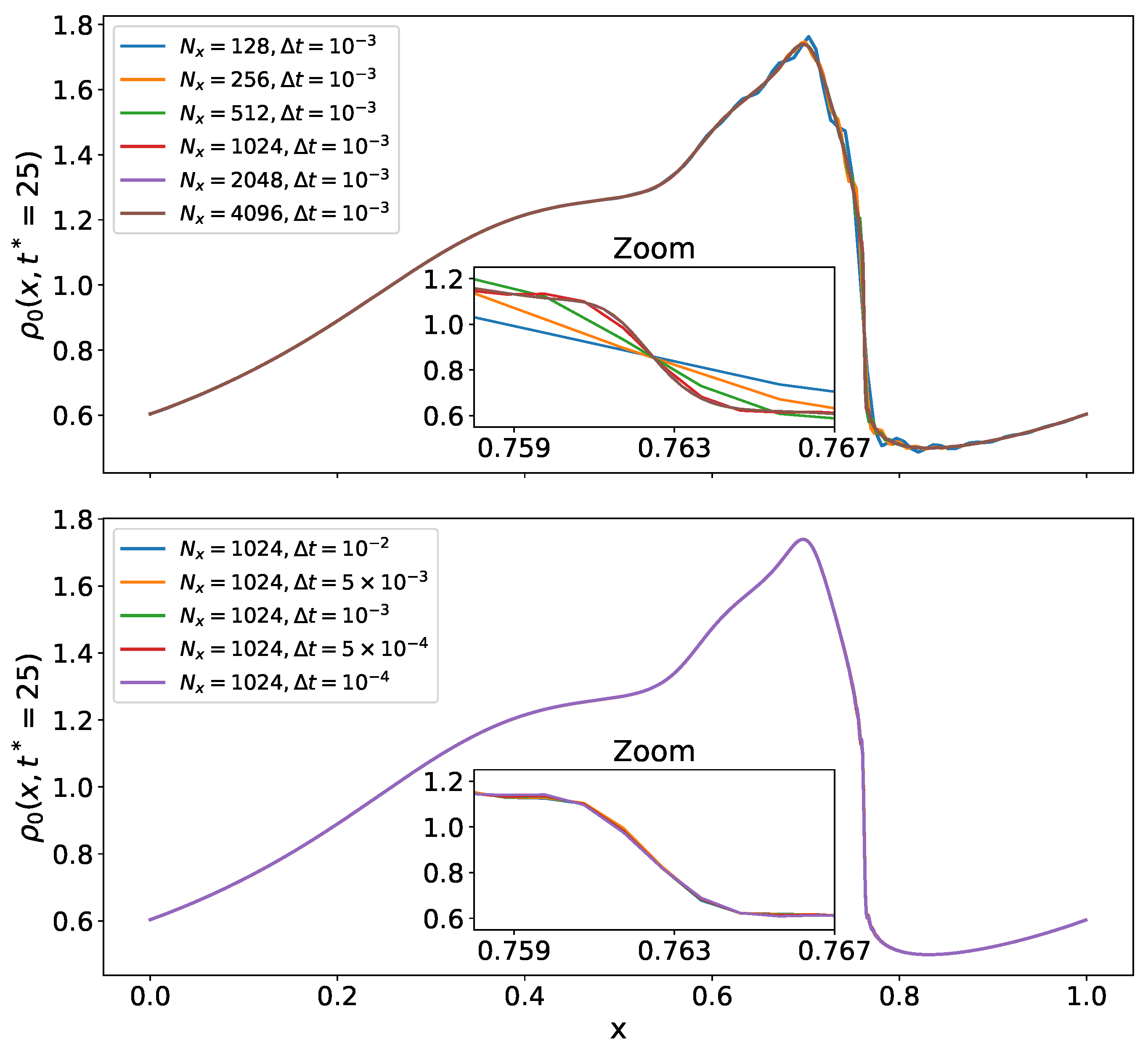
3.1. Propagation of Classical Sound Wave in Nonlinear Regime

To numerically address these challenges, we have integrated a dedicated module into the SFINGE code, following the details outlined in Section 2. We begin by considering the propagation of a classical one-dimensional sound wave in the nonlinear regime within a fixed and flat Minkowski spacetime. This scenario offers a simple yet rigorous benchmark for evaluating the method’s ability to preserve stability and accuracy in the presence of sharp gradients and discontinuities. To this end, we initialized the x-component of the three-velocity term as a monochromatic sound wave:
v x ( x , t ) = A c s sin ( k x ω t ) ,
where A = 0.5 is the amplitude, k = 2 π / L x is the wavenumber, and  L x = 1 is the size of the simulation box. Here, c s represents the phase velocity, equivalent to the classical sound speed ( c s c ), and it is defined as
c s = ω k = Γ P ˜ 0 ρ ˜ 0 = 10 2 ,
with unperturbed quantities ρ ˜ 0 = 1 and P ˜ 0 = 10 4 / Γ , where Γ = 4 / 3 denotes the adiabatic index. The rest-mass density and pressure are initialized as follows:
ρ 0 ( x , t ) = ρ ˜ 0 1 + A c s sin ( k x ω t ) ,
P ( x , t ) = P ˜ 0 1 + A c s sin ( k x ω t ) .
The objective is to evolve a clean shock wave free of spurious oscillations while ensuring numerical stability throughout the simulation. To this end, we seek to identify the optimal values of the anti-aliasing cut-off wavenumber k * used for spectral filtering and the dissipative coefficient ν 4 employed in the IHB method. Across all simulated configurations, the spatial and temporal resolutions are kept constant, with  N x = 2048 and Δ t = 10 3 , while k * and ν 4 are systematically varied. Each simulation is carried out up the shock formation stage, at which point the results are analyzed and compared.
Figure 1 shows the profiles of the numerically simulated wave velocity v x ( x , t * ) (top) and the rest-mass density ρ 0 ( x , t * ) (bottom) at t * = 25 . The grid resolution and time step are fixed, while the dissipation coefficient is varied from ν 4 = 10 13 to ν 4 = 5 × 10 12 , passing through intermediate values of ν 4 = 5 × 10 13 and ν 4 = 10 12 . Simultaneously, the filter cut-off was adjusted from k * = N x / 2.0 to k * = N x / 4.0 , with  k * = N x / 3.0 as an intermediate setting. Additionally, a reference case (blue line) is shown in which the hyperviscous scheme is not applied ( ν 4 = 0.0 ) and the filter acts on the minimal number of Fourier modes, specifically at k * = N x / 2.0 , corresponding to the Nyquist mode, which is dependent on the discretization. The figure also includes a magnified view of the shock region along the x-axis, highlighting differences among the configurations. For higher values of the dissipation coefficient, the wave is excessively damped, while for lower values, spurious ripples are not fully suppressed. The choice of filter cut-off appears to have minimal influence on the smoothness and cleanliness of the wave, particularly as ν 4 increases (note that the pink and brown lines almost perfectly overlap). Based on this analysis, the optimal parameters are identified as k * = N x / 3.0 and ν 4 = 10 12 , represented by the purple line.
Having selected the optimal filter and dissipation coefficient, we proceeded to perform a convergence test to assess the efficiency of the new code formulation. This involves evolving nonlinear classical sound waves while systematically refining the spatial and temporal resolution to assess the accuracy of the computed solutions. As depicted in Figure 2, we analyzed the convergence behavior of the rest-mass density ρ 0 . The results reveal clear convergence for spatial resolutions exceeding N x = 512 . In this regime, the red, purple, and brown lines in the top panel become nearly indistinguishable, indicating that further spatial refinement introduces negligible changes to the numerical solution. As for the temporal resolution, convergence is already achieved for time step sizes around Δ t = 10 2 . Indeed, all curves in the bottom panel exhibit a consistent and closely aligned trend, suggesting that temporal discretization errors are sufficiently minimized at these finer resolutions.

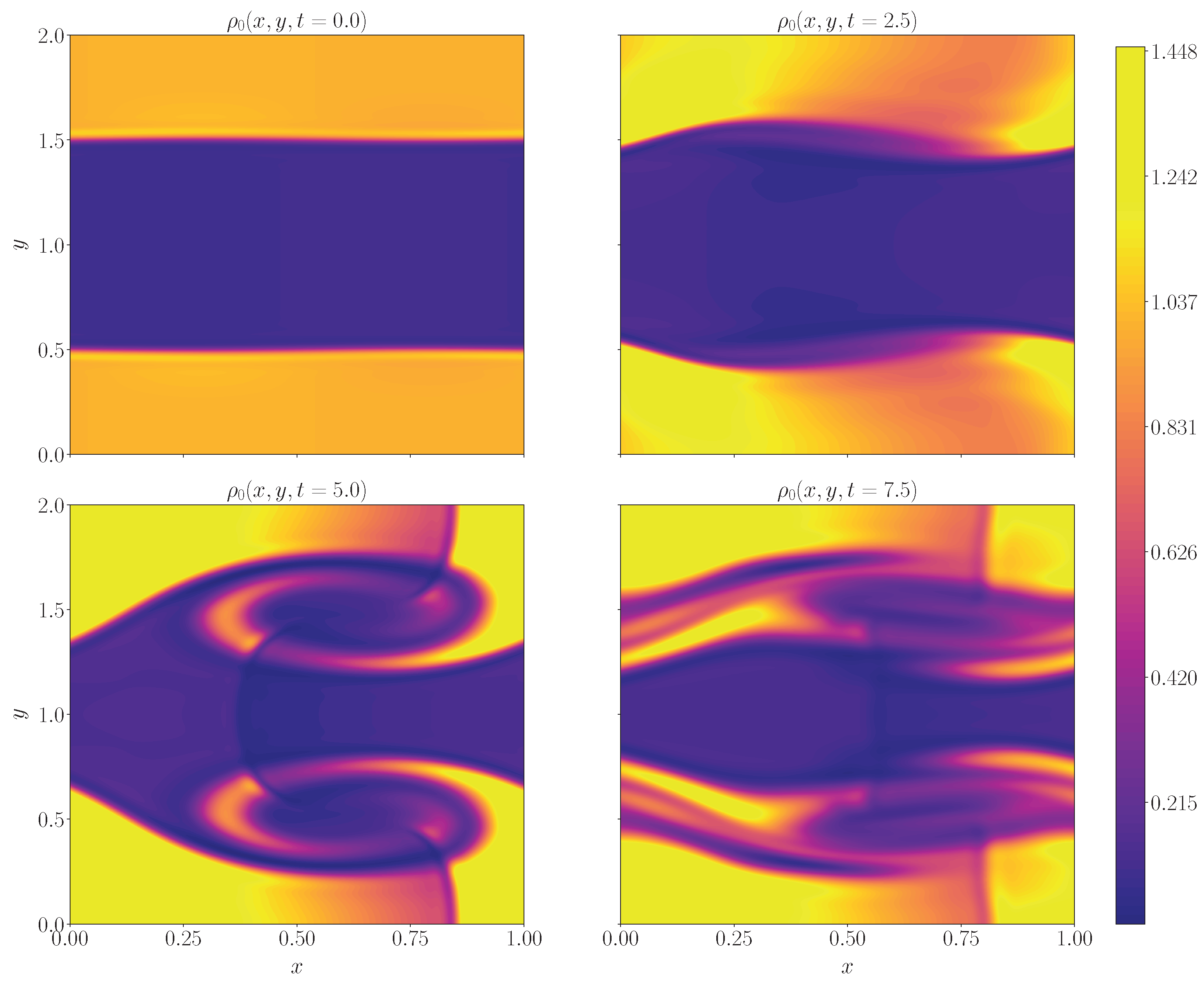
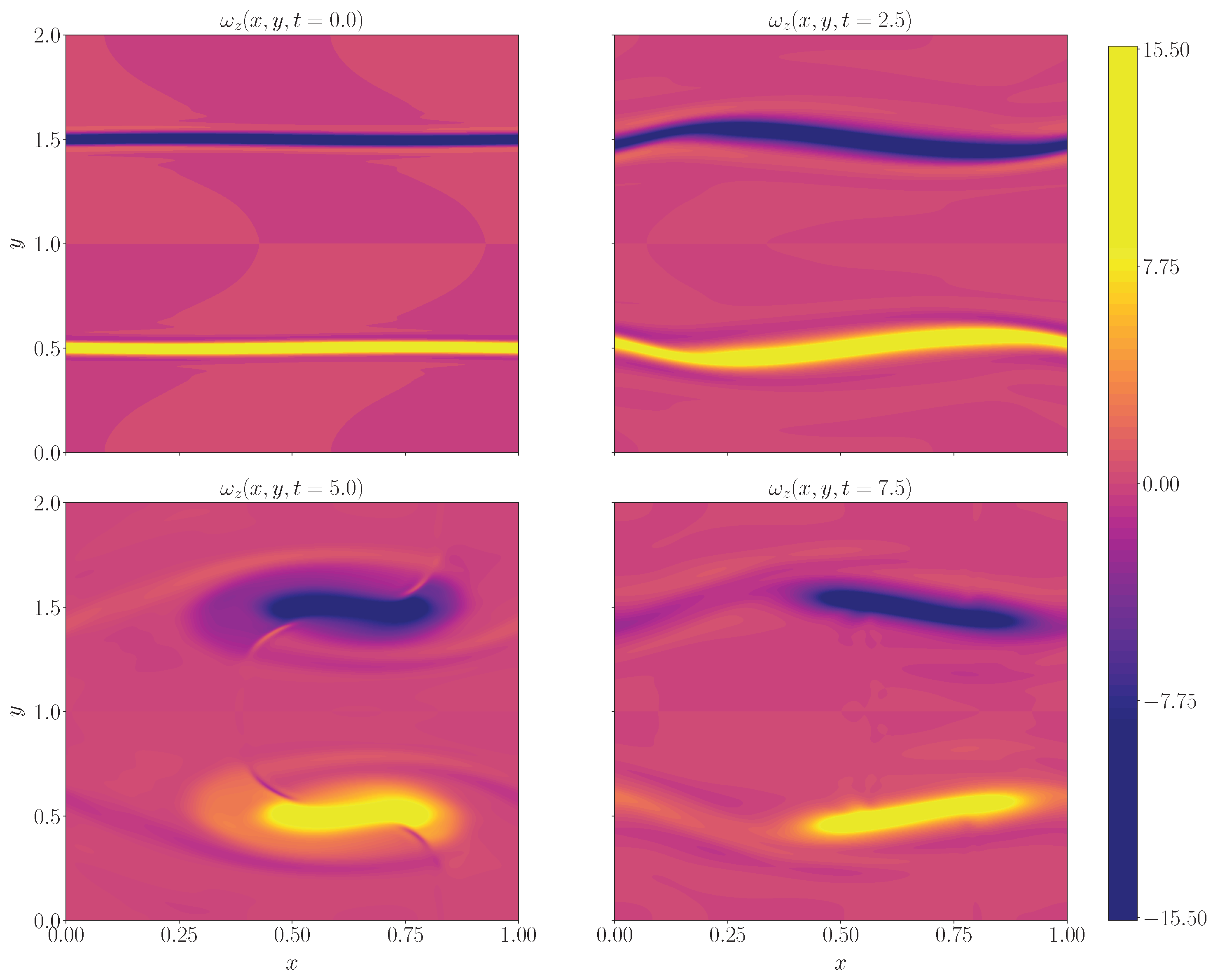
3.2. Kelvin–Helmholtz Instability

As a second test, we aimed to trigger the KHI within the framework of special relativity, following the setup described by Beckwith and Stone [48] and Radice and Rezzolla [49]. As is common in numerical studies, we adopted hyperbolic tangent profiles to smoothly capture the shear interface. To ensure periodic boundary conditions in both spatial directions, a double-hyperbolic-tangent profile was employed. The two-dimensional spatial domain is defined as x , y [ 0 , L x ] × [ 0 , L y ] , with  L x = 1 and L y = 2 , and it is discretized using a grid of N x × N y = 1024 × 2048 points. The velocity shear is imposed through the following profile:
v x ( y ) = v s tanh y y 1 a 0 tanh y y 2 a 0 1 ,
where a 0 = 0.01 denotes the thickness of the shear layer, v s = 0.5 represents the shear velocity amplitude, and the positions y 1 = 1.5 and y 2 = 0.5 define the shear layer. The initial velocity perturbation is expressed as
v y ( x , y ) = A exp 0.5 y y 1 σ 0 2 exp 0.5 y y 2 σ 0 2 sin 2 π x L x ,
with an amplitude of A = 10 1 v s . The rest-mass density is initialized as
ρ 0 ( y ) = 1 + 0.45 tanh y 1.5 a 0 tanh y 0.5 a 0 .
The simulation is performed up to t = 10 , allowing the characteristic Kelvin–Helmholtz rolls to fully develop and become clearly distinguishable. As shown in Figure 3, the onset of the instability in the rest-mass density becomes evident around t = 2.5 . The evolution closely matches the numerical results reported by Beckwith and Stone [48] and Radice and Rezzolla [49] for a single-mode perturbation. Figure 4 displays the only non-vanishing component of the vorticity, ω z = × v z = x v y y v x , which serves as a key diagnostic of rotational motion and shear amplification, highlighting regions of intense fluid rotation. It provides a clear picture of the transition from linear growth to nonlinear saturation, making it an essential tool for analyzing vortex dynamics and the energy cascade in shear flows. As can be inferred from the figure, the vorticity is initially concentrated along a narrow shear layer at the interface between two fluid layers moving with opposing velocities. As the instability develops, small-scale perturbations grow and roll up into coherent vortices, clearly visible as alternating regions of positive and negative vorticity. Remarkably, the full nonlinear development of the KHI is successfully captured using the logarithmic formulation of GRHD introduced in Section 2. This approach, applied here in the context of flat spacetime, enables a stable numerical treatment of the steep gradients that characterize the instability while also providing an efficient framework for simulating its complex nonlinear dynamics.
Future tests will incorporate the dynamical evolution of spacetime curvature to evaluate the performance of the code in scenarios where curvature and matter are fully coupled. This extension is intended to provide a comprehensive assessment of the robustness and accuracy of the numerical methods under more physically realistic conditions.

4. Discussion

In this study, we introduced a novel logarithmic formulation of the GRHD equations within the BSSN framework. The key innovation lies in transforming critical fluid variables into logarithmic space. This transformation not only preserves the positivity of fundamental quantities such as density and pressure but also helps mitigate steep gradients that commonly arise in highly dynamical spacetimes. This property is valuable for a wide range of astrophysical problems, such as the evolution of matter onto neutron stars and black holes, the merging dynamics of compact objects involving matter, and cosmological simulations, where the evolution of density perturbations in an expanding universe can lead to extreme variations in physical quantities [50,51,52].
The present formulation offers several advantages for the aforementioned applications. First, it provides a robust numerical framework for analyzing the nonlinear evolution of astrophysical systems beyond the linear perturbation regime. Second, when combined with spectral methods such as FFT and the IHB technique, our approach significantly reduces numerical noise and enhances the stability of long-term integrations. These features are important for capturing the intricate interplay between fluid dynamics and spacetime curvature, where conventional numerical schemes often suffer from instabilities or excessive diffusion.
Traditional perturbation methods, which rely on linearized approximations, typically break down when density contrasts become large, or they employ techniques that can result in a significant loss of information. In contrast, our logarithmic reformulation is expected to improve numerical stability and ensure physical consistency across vastly different density scales. This advantage may be particularly pronounced in regions where densities sharply decrease as a result of shock waves generated by plasma instabilities or small-scale cosmological evolution. By preserving the accuracy of simulations across a broad range of densities, our approach provides a promising framework even for cosmological studies, including investigations of inhomogeneous universes [53,54].
Furthermore, this logarithmic formulation may naturally extend to GRMHD simulations, unlocking new possibilities for exploring the role of primordial magnetic fields in structure formation and cosmic magnetism. This extension could enable a deeper understanding of high-energy cosmological phenomena, where magnetic effects play a non-negligible role.
For completeness, we present below the final system of GRHD equations in logarithmic form within the BSSN formalism, along with the subsequent definitions:
( t β k k ) γ ˜ i j = 2 α A ˜ i j + γ ˜ i k j β k + γ ˜ k j i β k 2 3 γ ˜ i j k β k ,
( t β k k ) A ˜ i j = χ α R ˜ i j + R ˜ i j χ 1 3 γ ˜ i j R i j α 1 3 γ ˜ i j k k α + α K A ˜ i j 2 A ˜ i k γ ˜ k l A ˜ l j + A ˜ i k j β k + A ˜ k j i β k 2 3 A ˜ i j k β k 8 π α χ D 0 e δ σ i v j + χ 1 γ ˜ i j e π TF ,
( t β i i ) K = γ ˜ i j i j α + α A ˜ i j A ˜ i j + 1 3 K 2 + 4 π α D 0 e δ + e ε + e δ σ i v i + 3 e π ,
( t β j j ) Γ ˜ i = γ ˜ j k j k β i + 1 3 γ ˜ i j j k β k Γ ˜ j j β i + 2 3 Γ ˜ i j β j 2 A ˜ i j j α + α 2 Γ ˜ j k i A ˜ j k 3 χ 1 A ˜ i j j χ 4 3 γ ˜ i j j K 16 π D 0 e δ σ i ,
( t β i i ) δ = α K α v i i δ i α v i ,
( t β j j ) σ i = 1 + e ε δ + e π δ χ γ ˜ i j j α e π δ α χ γ ˜ i j j π σ j j β i α v j j σ i ,
( t β i i ) ε = α v i i ε + α v i v j K i j v j j α + α K i α v i 1 + e π ε + α v i v j K i j e δ ε v j j α e δ ε e π ε α v i i π ,
where E = τ + D = D 0 e ε + e δ , S i = D 0 e δ σ i , and  S i j = D 0 e δ σ i v j + χ γ ˜ i j e π are expressed in their logarithmic form. In this set of equations, R represents the Ricci tensor trace, while R ˜ i j is the conformal Ricci tensor. The term R ˜ i j χ represents the contribution of the conformal factor such that the full spatial Ricci tensor is given by R i j = R ˜ i j + R ˜ i j χ .
The above set of equations defines the logarithmic formulation of the Einstein equations coupled with the hydrodynamic equations, where the application of FFT-based methods ensures high numerical accuracy, making it well-suited to address a broad range of astrophysical problems. By introducing this logarithmic framework [55], we aim to establish a more robust mathematical approach for modeling strong-field gravitational effects in the presence of matter. This method also seeks to improve our understanding of back-reaction effects, structure formation, and the large-scale dynamics of the universe. The logarithmic formulation departs from the strict conservation form, meaning that mass and energy are no longer conserved to machine precision. We found that for the one-dimensional nonlinear sound wave test described in Section 3, the relative loss of these quantities does not exceed 0.3 % . Future studies will assess how well mass and energy are conserved in the full GRHD framework and quantify the impact on numerical accuracy.

5. Conclusions

We have introduced a new logarithmic formulation of the GRHD equations within the BSSN formalism, with a specific emphasis on its relevance to key astrophysical problems, ranging from the dynamics of matter in curved spacetimes around compact objects to cosmological applications. By mapping some crucial fluid variables into logarithmic space, the proposed method is expected to mitigate numerical instabilities linked to steep gradients and to treat large variations in quantities such as pressure or mass and energy densities while ensuring their physical positivity. These characteristics are essential when simulating the highly nonlinear regimes encountered in such extreme environments.
The enhanced numerical stability and compatibility with high-precision spectral methods (e.g., FFT) make this approach a promising tool for tackling the challenges of simulating the evolution of cosmic flows and density perturbations in an expanding spacetime. Furthermore, its application to the study of the dynamics of matter around black holes, particularly in relation to gravitational wave emissions, may offer exciting prospects for multi-messenger astrophysics. The potential extension of this framework to include magnetohydrodynamic effects would also enable an investigation into the role of magnetic fields in the early universe and the evolution of cosmic magnetism.
Future studies will involve the integration of this formulation into advanced numerical relativistic codes (e.g, SFINGE) and comparing it with established simulations of black hole accretion disks, gravitational wave emissions, and matter dynamics in strong gravitational fields. We expect that the logarithmic approach could improve the accuracy of GRHD simulations in these extreme environments and better capture the fluid dynamics in strongly curved spacetimes, supporting a more accurate modeling of the gravitational wave signals produced in such systems. In addition, applying this method to cosmological scenarios, including comparisons between perturbed and unperturbed Friedmann–Lemaître–Robertson–Walker (FLRW) spacetimes within a matter-dominated cosmological model [54,56], will contribute to a better understanding of the evolution of cosmic flows and density perturbations. The framework, which may be extended to include GRMHD effects, could also shed light on the role of magnetic fields in both black hole accretion processes and the early universe, reinforcing the multi-messenger approach to astrophysical research.

Author Contributions

Conceptualization, L.D.Z. and S.S.; methodology, M.I., R.M., L.D.Z. and S.S.; validation, L.D.Z. and S.S.; formal analysis, M.I. and R.M.; investigation, M.I., R.M., L.D.Z. and S.S.; resources, S.S.; data curation, M.I., R.M., L.D.Z. and S.S.; writing—original draft preparation, M.I. and R.M.; writing—review and editing, M.I. and R.M.; visualization, L.D.Z. and S.S.; supervision, L.D.Z. and S.S.; project administration, M.I. All authors have read and agreed to the published version of the manuscript.

Funding

This research received no external funding.

Data Availability Statement

The original contributions presented in this study are included in the article. Further inquiries can be directed to the corresponding author.

Acknowledgments

We acknowledge C.F. Gammie for his valuable and insightful advice. This work was supported by ICSC-Centro Nazionale di Ricerca in High Performance Computing, Big Data and Quantum Computing, funded by the European Union—NextGenerationEU. Simulations were performed in the Alarico HPPC Computing Facility at the University of Calabria, using a parallel computing infrastructure based on MPI directives.

Conflicts of Interest

The authors declare no conflicts of interest.

Note

1
Pressure normalization should involve D 0 c 2 , which is the reference mass–energy density adopted for the normalization of the stress–energy tensor; yet this coincides with D 0 under the chosen units.

References

  1. Blandford, R.D.; Znajek, R.L. Electromagnetic extraction of energy from Kerr black holes. Mon. Not. R. Astron. Soc. 1977, 179, 433–456. [Google Scholar] [CrossRef]
  2. Blandford, R.D.; Payne, D.G. Hydromagnetic flows from accretion discs and the production of radio jets. Mon. Not. R. Astron. Soc. 1982, 199, 883–903. [Google Scholar] [CrossRef]
  3. De Villiers, J.P.; Hawley, J.F.; Krolik, J.H.; Hirose, S. Magnetically driven accretion in the Kerr metric. III. Unbound outflows. Astrophys. J. 2005, 620, 878. [Google Scholar] [CrossRef]
  4. Radice, D.; Perego, A.; Zappa, F.; Bernuzzi, S. GW170817: Joint constraint on the neutron star equation of state from multimessenger observations. Astrophys. J. Lett. 2018, 852, L29. [Google Scholar] [CrossRef]
  5. Baiotti, L.; Rezzolla, L. Binary neutron star mergers: A review of Einstein’s richest laboratory. Rep. Prog. Phys. 2017, 80, 096901. [Google Scholar] [CrossRef]
  6. Giacomazzo, B.; Perna, R. Formation of stable magnetars from binary neutron star mergers. Astrophys. J. Lett. 2013, 771, L26. [Google Scholar] [CrossRef]
  7. Fernández, R.; Tchekhovskoy, A.; Quataert, E.; Foucart, F.; Kasen, D. Long-term GRMHD simulations of neutron star merger accretion discs: Implications for electromagnetic counterparts. Mon. Not. R. Astron. Soc. 2019, 482, 3373–3393. [Google Scholar] [CrossRef]
  8. Ciolfi, R. Binary neutron star mergers after GW170817. Front. Astron. Space Sci. 2020, 7, 27. [Google Scholar] [CrossRef]
  9. Durrer, R.; Neronov, A. Cosmological magnetic fields: Their generation, evolution and observation. Astron. Astrophys. Rev. 2013, 21, 1–109. [Google Scholar] [CrossRef]
  10. Subramanian, K. The origin, evolution and signatures of primordial magnetic fields. Rep. Prog. Phys. 2016, 79, 076901. [Google Scholar] [CrossRef]
  11. Wilson, J.R. Numerical Study of Fluid Flow in a Curved Spacetime. Astrophys. J. 1972, 173, 431–444. [Google Scholar] [CrossRef]
  12. Font, J.A. Hydrodynamics in full general relativity: Formulations, implementations, and tests. Phys. Rev. D 2000, 62, 084017. [Google Scholar] [CrossRef]
  13. Shibata, M.; Sekiguchi, Y.I. Three-dimensional simulations of stellar core collapse in full general relativity: Nonaxisymmetric dynamical instabilities. Phys. Rev. D 2005, 71, 024014. [Google Scholar] [CrossRef]
  14. Arnowitt, R.; Deser, S.; Misner, C.W. Republication of: The dynamics of general relativity. Gen. Relativ. Gravit. 2008, 40, 1997–2027. [Google Scholar] [CrossRef]
  15. Shibata, M.; Nakamura, T. Evolution of three-dimensional gravitational waves: Harmonic slicing case. Phys. Rev. D 1995, 52, 5428–5444. [Google Scholar] [CrossRef]
  16. Baumgarte, T.W.; Shapiro, S.L. On the numerical integration of Einstein’s field equations. Phys. Rev. D 1999, 59, 024007. [Google Scholar] [CrossRef]
  17. Alcubierre, M.; Allen, G.; Brügmann, B.; Seidel, E.; Suen, W.-M. Towards a stable numerical evolution of strongly gravitating systems in general relativity: The Conformal Transverse-Traceless Decomposition. Phys. Rev. D 2000, 62, 124011. [Google Scholar] [CrossRef]
  18. Zlochower, Y.; Baker, J.G.; Campanelli, M.; Lousto, C.O. Accurate black hole evolutions by fourth-order numerical relativity. Phys. Rev. D—Part. Fields Gravit. Cosmol. 2005, 72, 024021. [Google Scholar] [CrossRef]
  19. Campanelli, M.; Lousto, C.O.; Marronetti, P.; Zlochower, Y. Accurate Evolutions of Orbiting Black-Hole Binaries Without Excision. Phys. Rev. Lett. 2006, 96, 111101. [Google Scholar] [CrossRef]
  20. Bardeen, J.M. Gauge-invariant cosmological perturbations. Phys. Rev. D 1980, 22, 1882. [Google Scholar] [CrossRef]
  21. Kodama, H.; Sasaki, M. Cosmological perturbation theory. Prog. Theor. Phys. Suppl. 1984, 78, 1–166. [Google Scholar] [CrossRef]
  22. Oliynyk, T.A. Cosmological Newtonian limit. Phys. Rev. D 2014, 89, 124002. [Google Scholar] [CrossRef]
  23. Räsänen, S. Applicability of the linearly perturbed FRW metric and Newtonian cosmology. Phys. Rev. D—Part. Fields Gravit. Cosmol. 2010, 81, 103512. [Google Scholar] [CrossRef]
  24. Adamek, J.; Daverio, D.; Durrer, R.; Kunz, M. gevolution: A cosmological N-body code based on General Relativity. J. Cosmol. Astropart. Phys. 2016, 2016, 053. [Google Scholar] [CrossRef]
  25. Tauber, J. et al. [ESA; The Planck Scientific Collaboration] The planck mission. Adv. Space Res. 2004, 34, 491–496. [Google Scholar] [CrossRef]
  26. Abbott, T.M.; Aguena, M.; Alarcon, A.; Allam, S.; Alves, O.; Amon, A.; Andrade-Oliveira, F.; Annis, J.; Avila, S.; Bacon, D.; et al. Dark Energy Survey Year 3 results: Cosmological constraints from galaxy clustering and weak lensing. Phys. Rev. D 2022, 105, 023520. [Google Scholar] [CrossRef]
  27. Laureijs, R.; Gondoin, P.; Duvet, L.; Criado, G.S.; Hoar, J.; Amiaux, J.; Auguères, J.L.; Cole, R.; Cropper, M.; Ealet, A.; et al. Euclid: ESA’s mission to map the geometry of the dark universe. In Proceedings of the Space Telescopes and Instrumentation 2012: Optical, Infrared, and Millimeter Wave, Amsterdam, The Netherlands, 1–6 July 2012; SPIE: Bellingham, DC, USA, 2012; Volume 8442, pp. 329–336. [Google Scholar]
  28. Palenzuela, C.; Lehner, L.; Ponce, M.; Liebling, S.L.; Anderson, M.; Neilsen, D.; Motl, P. Electromagnetic and gravitational outputs from binary-neutron-star coalescence. Phys. Rev. Lett. 2013, 111, 061105. [Google Scholar] [CrossRef] [PubMed]
  29. Dionysopoulou, K.; Alic, D.; Palenzuela, C.; Rezzolla, L.; Giacomazzo, B. General-relativistic resistive magnetohydrodynamics in three dimensions: Formulation and tests. Phys. Rev. D—Part. Fields Gravit. Cosmol. 2013, 88, 044020. [Google Scholar] [CrossRef]
  30. Ripperda, B.; Bacchini, F.; Porth, O.; Most, E.R.; Olivares, H.; Nathanail, A.; Rezzolla, L.; Teunissen, J.; Keppens, R. General-relativistic resistive magnetohydrodynamics with robust primitive-variable recovery for accretion disk simulations. Astrophys. J. Suppl. Ser. 2019, 244, 10. [Google Scholar] [CrossRef]
  31. Martí, J.M.; Müller, E. Numerical hydrodynamics in special relativity. Living Rev. Relativ. 1999, 2, 3. [Google Scholar] [CrossRef]
  32. Del Zanna, L.; Bucciantini, N. An efficient shock-capturing central-type scheme for multidimensional relativistic flows. Astron. Astrophys. 2002, 390, 1177–1186. [Google Scholar] [CrossRef]
  33. Imbrogno, M.; Meringolo, C.; Servidio, S. Extreme gravitational interactions in the problem of three black holes in general relativity. Class. Quantum Gravity 2023, 40, 075008. [Google Scholar] [CrossRef]
  34. Bona, C.; Massó, J. Einstein’s evolution equations as a system of balance laws. Phys. Rev. D 1989, 40, 1022. [Google Scholar] [CrossRef] [PubMed]
  35. Bona, C.; Masso, J.; Seidel, E.; Stela, J. New formalism for numerical relativity. Phys. Rev. Lett. 1995, 75, 600. [Google Scholar] [CrossRef] [PubMed]
  36. Alcubierre, M.; Allen, G.; Bona, C.; Fiske, D.; Goodale, T.; Guzmán, F.S.; Hawke, I.; Hawley, S.H.; Husa, S.; Koppitz, M.; et al. Towards standard testbeds for numerical relativity. Class. Quantum Gravity 2003, 21, 589. [Google Scholar] [CrossRef]
  37. Alcubierre, M. Introduction to 3 + 1 Numerical Relativity; Oxford University Press: Oxford, UK, 2008. [Google Scholar]
  38. Akbarian, A.; Choptuik, M.W. Black hole critical behavior with the generalized BSSN formulation. Phys. Rev. D 2015, 92, 084037. [Google Scholar] [CrossRef]
  39. Alekseenko, A.M. Constraint preserving boundary conditions for the linearized BSSN formulation. arXiv 2004, arXiv:gr-qc/0405080. [Google Scholar]
  40. Gundlach, C.; Martin-Garcia, J.M. Well-posedness of formulations of the Einstein equations with dynamical lapse and shift conditions. Phys. Rev. D—Part. Fields Gravitat. Cosmol. 2006, 74, 024016. [Google Scholar] [CrossRef]
  41. Brown, J.D. Covariant formulations of Baumgarte, Shapiro, Shibata, and Nakamura and the standard gauge. Phys. Rev. D—Part. Fields Gravitat. Cosmol. 2009, 79, 104029. [Google Scholar] [CrossRef]
  42. Mignone, A.; Bodo, G.; Massaglia, S.; Matsakos, T.; Tesileanu, O.; Zanni, C.; Ferrari, A. PLUTO: A Numerical Code for Computational Astrophysics. Astrophys. J. Suppl. Ser. 2007, 170, 228–242. [Google Scholar] [CrossRef]
  43. Baiotti, L.; Giacomazzo, B.; Rezzolla, L. Accurate evolutions of inspiralling and magnetized neutron stars: Equal-mass binaries. Phys. Rev. D 2008, 78, 084033. [Google Scholar] [CrossRef]
  44. Galeazzi, F.; Kastaun, W.; Rezzolla, L.; Font, J.A. Implementation of a simplified approach to radiative transfer in general relativity. Phys. Rev. D—Part. Fields Gravitat. Cosmol. 2013, 88, 064009. [Google Scholar] [CrossRef]
  45. Baiotti, L.; Pietri, R.D.; Manca, G.M.; Rezzolla, L. Accurate simulations of the dynamical bar-mode instability in full general relativity. Phys. Rev. D—Part. Fields Gravitat. Cosmol. 2007, 75, 044023. [Google Scholar] [CrossRef]
  46. Meringolo, C.; Servidio, S.; Veltri, P. A spectral method algorithm for numerical simulations of gravitational fields. Class. Quantum Gravity 2021, 38, 075027. [Google Scholar] [CrossRef]
  47. Meringolo, C.; Servidio, S. Aliasing Instabilities in the Numerical Evolution of the Einstein Field Equations. Gen. Relativ. Gravit. 2021, 53, 95. [Google Scholar] [CrossRef]
  48. Beckwith, K.; Stone, J.M. A second-order Godunov method for multi-dimensional relativistic magnetohydrodynamics. Astrophys. J. Suppl. Ser. 2011, 193, 6. [Google Scholar] [CrossRef]
  49. Radice, D.; Rezzolla, L. THC: A new high-order finite-difference high-resolution shock-capturing code for special-relativistic hydrodynamics. Astron. Astrophys. 2012, 547, A26. [Google Scholar] [CrossRef]
  50. Bertschinger, E. Simulations of structure formation in the universe. Annu. Rev. Astron. Astrophys. 1998, 36, 599–654. [Google Scholar] [CrossRef]
  51. Hahn, O.; Paranjape, A. General relativistic screening in cosmological simulations. Phys. Rev. D 2016, 94, 083511. [Google Scholar] [CrossRef]
  52. Zou, J.; Zhu, Z.; Zhao, Z.; Bian, L. Numerical simulations of density perturbation and gravitational wave production from cosmological first-order phase transition. arXiv 2025, arXiv:2502.20166. [Google Scholar]
  53. Adamek, J.; Daverio, D.; Durrer, R.; Kunz, M. General Relativistic N-body simulations in the weak field limit. Phys. Rev. D—Part. Fields Gravitat. Cosmol. 2013, 88, 103527. [Google Scholar] [CrossRef]
  54. Mertens, J.B.; Giblin, J.T., Jr.; Starkman, G.D. Integration of inhomogeneous cosmological spacetimes in the BSSN formalism. Phys. Rev. D 2016, 93, 124059. [Google Scholar] [CrossRef]
  55. Stein, R.F.; Nordlund, Å. Realistic solar convection simulations. Sol. Phys. 2000, 192, 91–108. [Google Scholar] [CrossRef]
  56. Macpherson, H.J.; Lasky, P.D.; Price, D.J. Inhomogeneous cosmology with numerical relativity. Phys. Rev. D 2017, 95, 064028. [Google Scholar] [CrossRef]
Figure 1. High-amplitude shock wave profiles for the x-component of the velocity (top) and the rest-mass density (bottom) at t * = 25 , displayed for different spectral filters k * and dissipative coefficients ν 4 . The inset provides a magnified view of the shock region, centered around x 0.76 , for both fields.
Universe 11 00194 g001
Figure 2. Spatial (top) and temporal (bottom) convergence tests for shock wave profiles of the rest-mass density ρ 0 at t * = 25 , presented for k * = 3.0 and ν 4 = 10 12 . The inset shows a magnified view of the shock region, centered around x 0.76 , for both tests.
Universe 11 00194 g002
Figure 3. Two-dimensional evolution of the rest-mass density.
Universe 11 00194 g003
Figure 4. Two-dimensional evolution of the z-component of the vorticity.
Universe 11 00194 g004
Disclaimer/Publisher’s Note: The statements, opinions and data contained in all publications are solely those of the individual author(s) and contributor(s) and not of MDPI and/or the editor(s). MDPI and/or the editor(s) disclaim responsibility for any injury to people or property resulting from any ideas, methods, instructions or products referred to in the content.

