Abstract
As an alternative gravitational theory to General Relativity (GR), Conformal Gravity (CG) can be verified through astronomical observations. Currently, Mannheim and Kazanas have provided vacuum solutions for cosmological and local gravitational systems, and these solutions may resolve the dark matter and dark energy issues encountered in GR, making them particularly valuable. For static, spherically symmetric systems, CG predicts an additional linear potential generated by luminous matter in addition to the conventional Newtonian potential. This extra potential is expected to account for the observations of galaxies and galaxy clusters without the need of dark matter. It is characterized by the parameter , which corresponds to the linear potential generated by the unit of the solar mass, and it is thus a universal constant. The value of was determined by fitting the rotation curve data of spiral galaxies. These predictions of CG should also be verified by the observations of strong gravitational lensing. To date, in the existing literature, the observations of strong lensing employed to test CG have been limited to a few galaxy clusters. It has been found that the value of estimated from strong lensing is several orders of magnitude greater than that obtained from fitting rotation curves. In this study, building upon the previous research, we tested CG via strong lensing statistics. We used a well-defined sample that consisted of both galaxies and galaxy clusters. This allowed us to test CG through statistical strong lensing in a way similar to the conventional approach in GR. As anticipated, our results were consistent with previous studies, namely that the fitted is much larger than that from rotation curves. Intriguingly, we further discovered that, in order to fit the strong lensing data of another sample, the value of cannot be a constant, as is required in CG. Instead, we derived a formula for as a function of the stellar mass of the galaxies or galaxy clusters. It was found that decreases as increases.
1. Introduction
According to General Relativity (GR), gravity can be characterized by the curvature of spacetime. The curvature of spacetime is dictated by the matter distribution within it. Test objects, and even light, traverse along the geodesics in the curved spacetime. As a result, if light passes near a massive object, such as a star, a galaxy, or a galaxy cluster, the bending of light will occur. This phenomenon is known as gravitational lensing. Now, gravitational lensing has evolved into an independent and powerful tool for constraining or examining the matter distribution profile and cosmological parameters in the standard CDM cosmology, as cited in [1]. On the other hand, GR turns out to be accurate only at the scales of a solar system. This includes its successful prediction of the deflection angle when distant light rays pass the edge of the sun. This prediction, also known as one of the three classic tests of GR, represents the earliest successful application of gravitational lensing [2]. At larger scales, including the whole universe, dark matter (DM) and dark energy (DE) must be introduced to ensure that GR remains a valid theory of gravity. However, as DM and DE still lack credible theoretical underpinnings and direct empirical evidence, numerous alternative gravity theories to GR have been developed. These alternative theories must undergo the scrutiny of astronomical and cosmological observations, including gravitational lensing. Conformal Gravity (CG) [3] is one such alternative theory.
Conformal Gravity (CG) has gained increasing attention as a potential alternative to dark matter (DM) and dark energy (DE), with its predictions being actively tested against astronomical observations [3]. As a relativistic theory extending beyond General Relativity (GR), CG offers solutions to both the cosmological constant problem inherent in CDM cosmology [4,5,6] and it demonstrates consistency with Type Ia supernova data [3,7].
In the non-relativistic limit, CG predicts a modified linear gravitational potential that supplements the Newtonian potential [8], potentially explaining galactic rotation curves without invoking DM. Recent studies have extensively tested this framework through detailed fits to observed the rotation curves of spiral galaxies [9,10,11]. These results consistently indicate a universal constant m−1, corresponding to the linear potential generated by a solar–mass () point source. For an arbitrary mass M, the linear potential scales as , where parametrizes the strength of this contribution.
Strong gravitational lensing has emerged as a valuable test for Conformal Gravity (CG), attracting growing research interest. While several studies [12,13,14,15,16,17] have derived light deflection angle expressions and performed lensing analyses in Mannheim–Kazanas spacetimes, the reported bending angle formulae show significant discrepancies and fail to converge. To date, tests of Conformal Gravity (CG) through strong lensing have been limited to individual galaxy clusters. In this work, we expanded the analysis to some well-defined samples of both galaxies and galaxy clusters. This approach enables systematic constraints on the parameter via strong lensing statistics, while probing for potential correlations between and the lens mass (M).
This paper is organized as follows: Section 2 reviews key Conformal Gravity (CG) results relevant to our analysis. Section 3 derives the CG deflection angle for lensing systems. In Section 4, the parameter is re-fitted using strong gravitational lensing data. We then present the galaxy stellar mass function in Section 5, which is followed by the lensing probability distribution fits for in Section 6. Finally, Section 7 provides the conclusions and discussion.
2. Cosmology and Galacdynamics in CG
Similar to General Relativity (GR), Conformal Gravity (CG) is formulated by taking the metric as the gravitational field. Nevertheless, it bestows an extra local symmetry upon gravity, namely the conformal symmetry , which surpasses the ordinary coordinate invariance. The Weyl tensor , defined by [3],
is conformal. It is constructed by a particular combination of the Riemann tensor , Ricci tensor and the Ricci scalar . The particular property of Weyl tensor is that it has the kinematic relation . In other words, the Weyl tensor is traceless.
By imposing the principle of local conformal invariance as the requisite principle to restrict the choice of action for the gravitational field in curved spacetime, one requires the uniquely selected fourth-order gravitational action [8]
to remain invariant under any local metric transformation, where is a dimensionless coupling constant. Variation of the action of Equation (2) with respect to the metric yields
where
Conformal gravity requires the energy-momentum tensor to be traceless, i.e., . On the other hand, elementary particle masses are not kinematic, but rather that they are acquired dynamically by spontaneous breakdown. Hence, consider a massless, spin- matter field fermion , which is to obtain its mass through a massless, real spin-0 Higgs scalar boson field . The required matter field action can be defined, as was done by [9], as
where h and are dimensionless coupling constants, are the Dirac matrices, and are the fermion spin connection. Variation of the matter action with respect to the metric yields matter the source energy–momentum tensor
The variation of the total action with respect to the metric yields the equation of motion for CG
To date, however, the exact solutions to Equation (7) can only be obtained for scenarios where . The difficulty stems from the fact that, in CG, when , we require an explicit dynamical model to describe how the gravitating system acquires its mass [8,18]. Therefore, in what follows, we will restrict our focus to the vacuum solutions where .
To test Conformal Gravity (CG) using galaxy observations and gravitational lensing data, we must solve Equation (7) for both cosmological scenarios and a static, spherically symmetric system.
In applying CG to cosmology, Weyl tensor vanishes in a Robertson–Walker metric [4]
Thus , and we can see from Equation (7) that . It turns out that conformal symmetry forbids the presence of any fundamental cosmological term, and is thus a symmetry which is able to control the cosmological constant. Even after the spontaneous breaking of conformal symmetry (which is required for particle mass generation), the induced cosmological constant’s contribution to cosmology remains controlled [3]. The full content of the theory can be obtained by choosing a particular gauge in which the scalar field takes the constant value . As a result, the energy–momentum tensor of Equation (6) becomes [19]
The averaging of over all the fermionic modes propagating in a Robertson–Walker background reduces the fermionic contribution to , i.e., to that of a kinematic perfect fluid
Thus, the conformal cosmology equation of motion can be written as [3]
When comparing with the standard Einstein equation in CDM model
we only need to replace the gravitational constant G by an effective, dynamically induced one . We defined the conformal analogs of the standard , and via
where is the Hubble parameter, and . As usual, a Robertson–Walker geometry Equation (7) yields, at redshift z, the expression of the Hubble parameter
where , etc. In subsequent calculations, we adopted the values , , and H0 = 69.3 km s−1 Mpc−1, as per reference [7].
For future reference, we defined the angular diameter distance as
where
The proper distance is
For a static, spherically symmetric gravitational system, it turns out that the full kinematic content of CG is contained in the line element [20]
Calculating for this line element leads to
Defining a source function
the equations of motion of Equation (7) can be written as
The exterior solution to Equation (21), with a radius of , is extremely important for the applications of CG to strong lensing and galactic dynamics [3,8]:
where the term is the general solution to the homogeneous equation . On defining
ignoring the term, and setting , the metric of Equation (22) can be written
When compared with the Schwarzschild solution in General Relativity (GR), the term corresponds to the conventional Newtonian potential. The term, on the other hand, represents an additional linear potential that is characteristic of Conformal Gravity (CG). The presence of this term enables CG to predict the rotation curves of spiral galaxies and the deflection angle of gravitational lensing without the need to invoke dark matter.
It is convenient to rewrite Equation (24) in terms of the potential . The rewritten form is as follows
In the region where , when , the Schwarzschild solution can be recovered. Departures from this solution, specifically the linear potential , only occur at large distances. For a typical star of the solar mass , we write its potential as
where m and can be determined by observations. If we denote , , and , then, for any point mass M, the expression for its potential shown in Equation (25) can be rewritten as
Here, is a universal constant introduced through the fitting of spiral galaxy rotation curves. It does not depend on the mass distribution of any particular galaxy and is interpreted as the effective manifestation of the global geometry of the universe—especially the negative spatial curvature—within a local coordinate system. This corresponds to a universal linear gravitational potential term arising from the Hubble flow. Its physical origin reflects the global properties of the universe under the conformal metric, rather than the gravitational contribution from individual matter sources [21].
We would like to point out that since represents the linear potential associated with a unit of luminous mass, its value ought to be a universal constant. In fact, through fitting the rotation curves of spiral galaxies, as reported in reference [3], it has been found that
Furthermore, as demonstrated in the above analysis, is regarded as a fixed constant across all galaxies. Throughout the remainder of this paper, we consistently adopt the value of as specified earlier. Consequently, unless otherwise noted, all references to the MK parameter in this work specifically refer to .
In the subsequent analysis, we aim to estimate the value of using a statistic strong lensing approach.
3. Deflection Angle and Lensing Equation
The deflection angle of the light path in a given metric of Equation (18) around a point mass is derived by solving the null geodesic equation in the equatorial plane of the lensing object
where , and the integration constant b can be expressed in terms of the distance of closest approach , which satisfies . The function is provided in the combined Equations (25) and (27). The deflection angle is derived by integrating from the closest approach of the light path to the horizon . The closest point is defined by , and the horizon is defined by . Thus, the deflection angle is given by
The integral can be evaluated after a series expansion of the integrand to the second order in . We, thus, obtain [17]
In Conformal Gravity (CG), the lensing equation has the same form as in General Relativity (GR). For a point mass lens, we have
where , , and are the source position angle, image position angle, and deflection angle of Equation (31), respectively; is closest approach of light path from the lens; , , and are the angular diameter distances from the observer to the lens, to the source, and from the lens to the source, respectively. Specifically, by setting in the lensing Equation (32), one can solve for the critical angular solution , which is known as the Einstein radius . This angle corresponds to the formation of a ring-like image when the background source, the lens, and the observer are perfectly aligned, satisfying the critical condition for multiple imaging.
4. Fitting the via Strong Gravitational Lensing
Mannheim [3] determined the standard value of the linear potential parameter by fitting the rotation curves of spiral galaxies (see Equation (28)). However, without invoking dark matter, Ghosh et al. [22] applied this parameter to analyze the strong lensing phenomena observed in the galaxy clusters Abell 370 and Abell 2390. They found that CG, under the standard value of , fails to reproduce the observed lensing effects. This discrepancy suggests that the value of obtained from rotation curve fits may not be sufficient to account for strong gravitational lensing, thereby motivating the need to refit within lensing systems. As can be seen from the deflection angle Formula (31) and the lensing Equation (32), if the observational data provide the redshifts of the background source and the lensing object , the Einstein radius , and the luminous mass enclosed within this radius , then the corresponding value of can be inferred. In this direction, related investigations have already been conducted by Cutajar and Zarb Adami [23].
After calculating the total linear potential parameter for each lensing system in their strong lensing galaxy cluster sample—where —they performed a fit to explore the correlation between and the gas mass . The results revealed a pronounced negative correlation between and . More critically, the magnitude of was found to be several orders of magnitude larger than the values obtained from rotation curve fits (for instance, the minimum value of obtained from their fitting satisfied the relation ). However, it is worth noting that all deflection angle expressions adopted in that study omitted the crucial second-order term , as compared to Equation (31). This omission could be a key factor contributing to the overestimated fit results. To further assess the impact of this missing term, we adopted the more complete deflection angle expression given by Equation (31), and we refitted the relation between and the mass. The use of here was intended to allow for a direct comparison with the values derived from rotation curve analyses.
We performed the fitting using the strong gravitational lensing sample compiled by Oguri et al. [24] (see Table 1). This sample provides key observational quantities, including the effective radius , the Einstein radius , and the total stellar mass , which are estimated under the assumption of a Salpeter initial mass function (IMF). Since the deflection angle calculated in the point-mass model (see Equation (31)) includes the Schwarzschild term , where M denotes the stellar mass enclosed within radius , we restricted our fitting of to the luminous mass enclosed within the Einstein radius, . This approach is consistent with the treatment in Cutajar and Zarb Adami [23], who also considered only the mass within the Einstein radius. It is important to emphasize that, unlike the Newtonian potential, the linear potential term in Conformal Gravity exhibits a non-local character. Specifically, the luminous mass located outside the Einstein radius does not produce mutually canceling gravitational effects at ; instead, it continues to contribute to light deflection. Therefore, by fitting using only the mass within , the gravitational effects of the external mass are effectively absorbed into an elevated value of , leading to an overestimation of this parameter. Nevertheless, such an overestimation does not alter the order of magnitude of . Thus, the fitted values obtained through this method remain valid for subsequent analyses.

Table 1.
The original parameters and fitting parameters in strong gravitational lens systems. From Column 1 to Column 7: galaxy name, source redshift , lens redshift , effective angular radius , Einstein radius , stellar mass , and the MK parameter .
In the framework of Conformal Gravity, where dark matter is not introduced, we modeled the distribution of luminous matter in the lensing object using the Hernquist density profile. The volume mass density was given by
where denotes the total stellar mass of the system, and is the scale radius, which is empirically related to the effective radius of the lensing galaxy by [25]. By adopting the transformation , the three-dimensional mass distribution can be recast in terms of angular coordinates. The stellar mass enclosed within an angular radius is then given by
where and denote the effective angular radius of the lensing object.
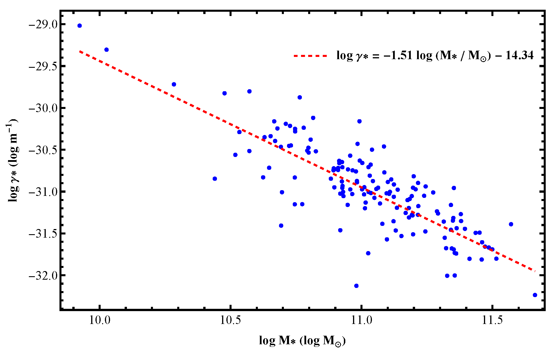
Using the observational data listed in Table 1, we calculated the value of for each lensing system by substituting into the lensing Equation (32) under the condition . Given that is a universal constant determined by the cosmological background and remains the same across all systems, we fixed its value as . The computed values of were plotted in Figure 1. Following the method adopted by Cutajar and Zarb Adami [23], we performed a least-squares fit to examine the empirical relation between and the stellar mass enclosed within the Einstein radius. The resulting fitting formula was given by
To distinguish this result from the standard parameter value derived from spiral galaxy rotation curves, we denoted the fitting result from strong lensing as . Compared to the findings of Cutajar and Zarb Adami [23], our obtained was significantly lower, yet it still remained substantially higher than the value inferred from galactic rotation curve fitting.
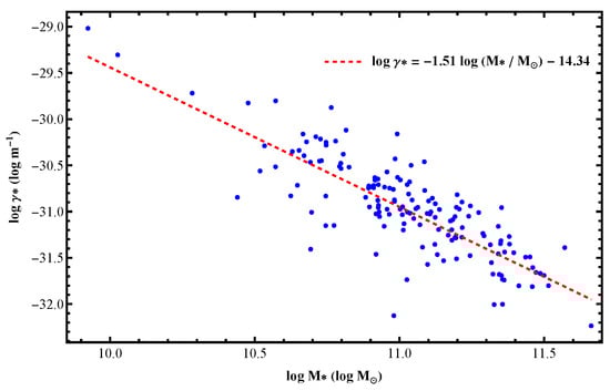
Figure 1.
A plot showing the relation between the Mannheim–Kazanas linear potential parameter and the stellar mass within the Einstein radius, which was derived from strong gravitational lensing observations. The data points represent individual lensing systems, and the dotted line denotes the empirical best-fit result.
In the following section, we will perform a statistical analysis of the lensing probability distribution based separately on and in order to further assess the explanatory power of different parameterizations with respect to the observational sample.
5. Galaxy Stellar Mass Function
To obtain the lensing probability within the framework of Conformal Gravity (CG), the galaxy stellar mass function (GSMF) is needed. It has been shown that, in different redshift ranges, choosing either a Schechter function [26],
or a double Schechter function [27],
can provide a good fit to the GSMF, where denotes the comoving number density of galaxies with mass between M and , is the normalization factor, and and are characteristic stellar mass of galaxies and the low-mass slope, respectively. Relying on the photometric data in the near-IR bands of the COSMOS2015 catalog and correcting the Eddington bias, Davidzon et al. [28] measured the GSMF in the redshift range of . This was achieved using a Schechter function and double Schechter function, as presented in Table 2. For galaxies with a redshift , Li and White [29] utilized a complete and uniform sample of 486,840 galaxies from the Sloan Digital Sky Survey to characterize the galaxy stellar mass function (GSMF) by fitting a Schechter function. They reported two sets of resulting parameters: one set was fitted in different stellar mass intervals, and the other was fitted across the entire mass range. Although the latter approach might overestimate the abundances of very massive galaxies, the number density of such galaxies is extremely low. Consequently, it has little impact on the prediction of the lensing probability. For convenience, in this study, we adopted the GSMF fitted across the entire mass range to describe galaxies with . The specific parameter values are also presented in Table 2.
Table 2.
The Schechter parameters across different redshift ranges. The parameter values for are cited from Li and White [29]. These values were obtained by fitting a Schechter function, and the reduced Hubble constant was adopted. For the redshift range , the parameter values were sourced from the reference Davidzon et al. [28]. Specifically, for , the values were fitted using a double Schechter function, while, for , a single Schechter function was used for fitting. In this case, the corresponding value of .
6. Lensing Probability
As previously mentioned, within the framework of Conformal Gravity (CG), we can only model the lens as a point mass. Despite the additional linear potential, namely the term, the lensing equation for a point mass in CG does not differ significantly from that in General Relativity (GR), as can be seen from Equations (31) and (32). In Figure 2, we present a typical lensing equation for a point luminous mass of . The source and the lens are located at redshifts and , respectively. As depicted, analogous to the situation in GR, a point-mass lensing system always has two images. We also found that, when , . Since the brightness of an image decreases as it gets closer to the lens and vice versa, the flux density ratio between the two brighter and fainter images increases as increases. On the other hand, any strong lensing sample has an allowed upper limit for , which leads to a corresponding upper limit of for each lensing system.
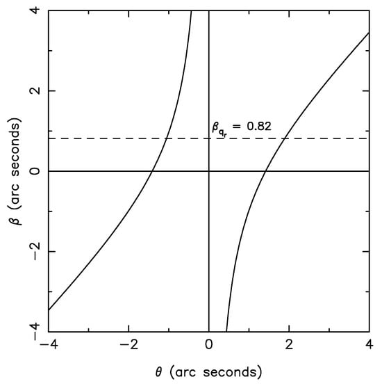
Figure 2.
The lensing Equation (32) for a point luminous mass of . The parameters were set as m−1, , and . The horizontal dashed line represents the allowed value of , which is constrained by the largest flux density ratio of the sample that was used in ref. [30].
In this study, we utilized the strong lensing sample presented in reference Inada et al. [30]. In this sample, the magnitude difference between the two brighter and fainter images in the i-band was restricted to mag, which implies . The magnifications of the two images are defined by
where are the two solutions of the lensing equation , corresponding to the angular positions of the two images. The flux density ratio is defined by . Specifically, we have
Here, represents the solution of the lensing equation on the negative half axis. Thus, can be obtained by solving the combined Equations (39) and (32).
In addition, gravitational lensing can magnify the brightness of background sources, such as quasars or galaxies. As a result, sources that would otherwise lie below the detection threshold (i.e., too faint to be observed) may be magnified above that threshold, thereby increasing their probability of being detected in survey samples. This leads to an observed number of lensing systems that exceeds the statistical expectation in the absence of lensing. On the other hand, magnification also stretches the image of the background object, effectively enlarging the observed area on the sky and thus reducing the surface number density of sources per unit solid angle. The net effect, known as magnification bias, is a combination of these two competing influences [31]. The expression for the magnification bias for a source at redshift and intrinsic luminosity L, under the effect of gravitational lensing, is given by [32,33]:
where is the luminosity function of the source population at redshift , is the lensing magnification factor, and characterizes the radial scale of the strong lensing region. A CLASS survey found that the number density of background sources follows a simple power–law relation . By fitting the number–flux relation of flat-spectrum sources with flux densities in the range at a frequency of , Rusin and Tegmark [34] determined the best-fit slope to be . In general applications, this parameter is typically taken as . With this simplification, Equation (40) reduces to the following:
where denotes the total magnification factor [32,33].
The lensing cross section is a central concept in the theory of statistical gravitational lensing, and it is used to quantify the effective area covered by a lensing system under specific imaging conditions. More precisely, it describes the area on the source plane in which a source satisfies a given imaging criterion—such as the production of multiple images, an image separation larger than a certain threshold, or a flux ratio below a specified value—for a fixed lens–source geometry. The cross section on the source plane for systems producing image separations greater than is defined as where is the caustic radius on the source plane corresponding to multiple imaging, is the image separation produced by a lens with mass M, and is the Heaviside function, which is defined as
For practical purposes, the lensing cross section is often transformed from the source plane to the lens plane. Using geometric relations, one obtains the following: which leads to the expression for the lensing cross section on the lens plane
This expression is of fundamental importance in the statistical prediction of strong gravitational lensing probabilities.
A lensing cross section with an image separation larger than and a flux density ratio less than , when combined with the amplification bias , is [35,36]
where is the source position at which a lens produces the image separation ; is the separation of the two images that are just on the Einstein ring; is the upper limit of the separation above which the flux ratio of the two images will be greater than ; andc is defined as the product of the lensing cross section and the magnification bias .
At last, in Conformal Gravity (CG), the lensing probability for QSOs at a mean redshift , which is lensed by foreground point-mass objects with image separations greater than and flux density ratios below , is given by
where the proper distance is provided in Equation (17), and the comoving number density can be selected from the galaxy stellar mass function (GSMF) fitted using a single Schechter function [Equation (36)] or double Schechter function [Equation (37)].
We utilized the final statistical sample of gravitationally lensed quasars from the Sloan Digital Sky Survey (SDSS) Quasar Lens Search (SQLS) [30]. This well-defined sample comprises 26 lensed quasars, with i-band magnitudes brighter than 19.1 and redshifts between 0.6 and 2.2, and they were selected from 50,826 spectroscopically confirmed quasars in SDSS Data Release 7 (DR7). The sample is restricted to systems with image separations of and i-band magnitude differences of less than 1.25 mag between the two images. For this lensed quasar sample, we adopted a mean source redshift of and constrained the flux density ratio to (corresponding to i-band magnitude differences mag) in our lensing probability calculations.
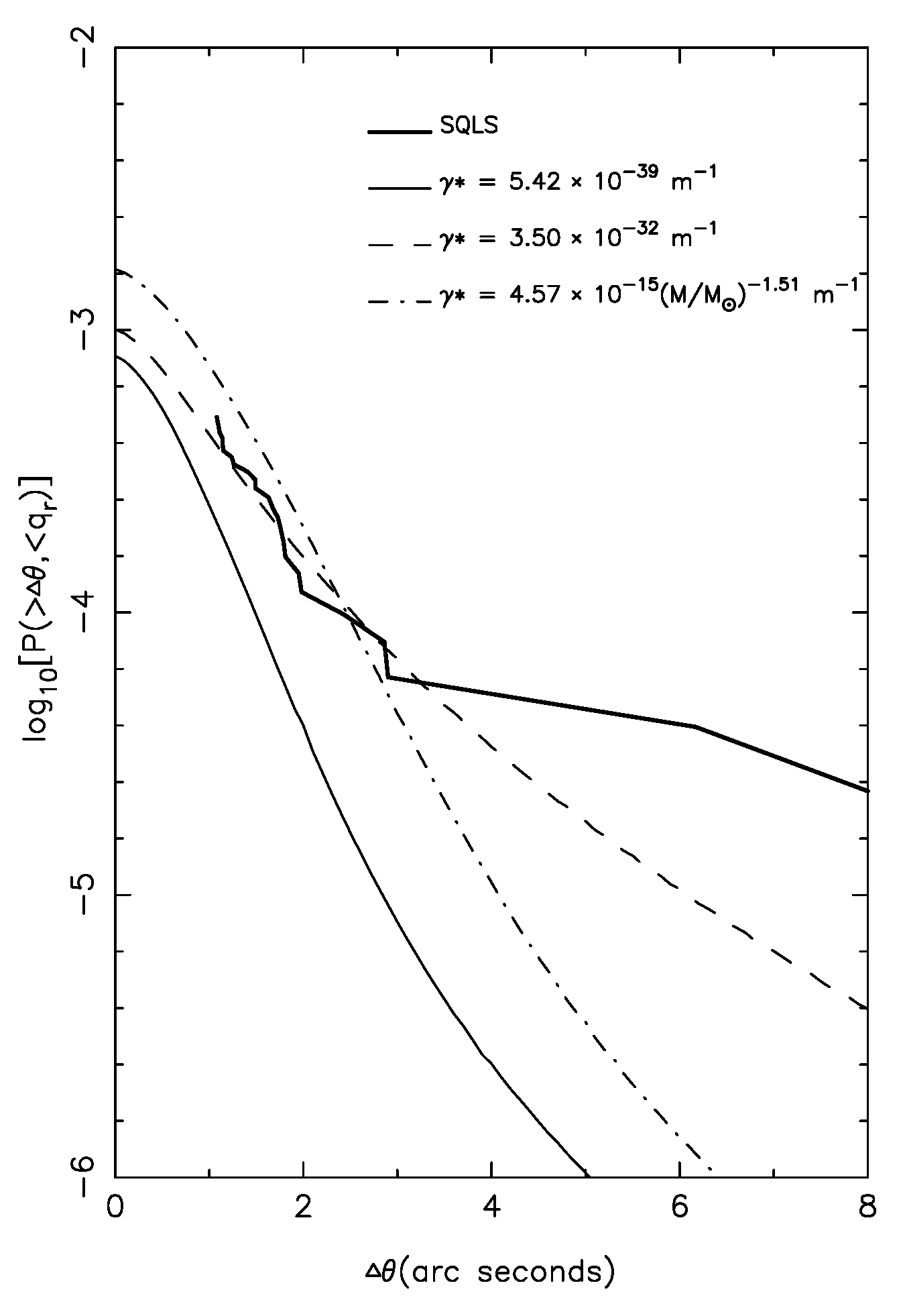
The parameter was constrained by fitting the lensing probability distribution predicted by Equation (44) to observations. Figure 3 presents the fitting results. The observed probability (thick histogram) was derived from the Inada et al. [30] sample through . The thin solid line shows the lensing probability prediction using the rotation-curve-derived standard value m−1 [3]. This significantly underestimates the observed distribution (thick histogram), and it is consistent with single-cluster studies [23].
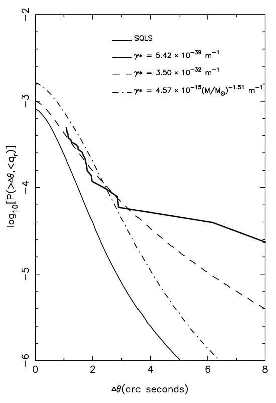
Figure 3.
Lensing probability with image separations and flux density ratios . The thick histogram shows the observed distribution from the Inada et al. [30] sample. The theoretical predictions are shown for the following: a standard rotation-curve-derived m−1 (thin solid line; [3]); obtained from strong gravitational lensing fits m−1 (dash-dotted line); and a best-fit constant m−1 (dashed line).
The dot-dashed line represents the predicted probability distribution of strong gravitational lensing under Conformal Gravity when the MK parameter is set to the best-fit value . It can be seen that, in the region of small image separations , the theoretical prediction lies above the observed distribution. This behavior is consistent with our earlier analysis: since the point-mass lens model neglects the non-local contribution of stellar mass located outside the Einstein radius to the linear potential term, the fitted value of is naturally elevated to compensate for the missing contribution. As a result, the predicted lensing probability is overestimated in the small-separation regime. In addition, a more important factor is the negative correlation between and the lens mass: lower-mass lenses tend to yield larger fitted values of . This enhances the contribution of the linear potential term in the deflection angle, increases the lensing cross section, and, consequently, amplifies the lensing probability for low-mass systems in the small-separation regime. In contrast, for image separations , the theoretical prediction from Conformal Gravity falls significantly below the observed distribution. A major reason for this discrepancy lies in the fact that the fitted decreases with increasing lens mass. For massive galaxies or galaxy clusters, the corresponding linear potential coefficient becomes smaller, thereby weakening the deflection angle and reducing the lensing probability.
For further comparison, we also plotted the predicted lensing probability distribution by assuming a constant , which is shown as the dashed line in the figure. The assumption of a constant is consistent with the fundamental premise of Conformal Gravity, wherein is taken to be the linear potential coefficient associated with a unit solar mass (for a detailed discussion, see Mannheim [3]). The best-fit constant MK parameter was found to be
As shown in Figure 3, when the image separation is , the strong lensing probability predicted by Conformal Gravity with a constant MK parameter is lower than that obtained using the mass-dependent parameter . In contrast, for , the prediction based on exceeds that of . This trend is consistent with our earlier analysis. However, when compared with the observational data, it is evident that Conformal Gravity underpredicts the strong lensing probability that occurs at large image separations, regardless of the form of adopted. Even when is tuned to its best-fit constant value from the data, the current formulation of Conformal Gravity remains insufficient to fully account for the observed strong lensing probability distribution.
Wang et al. [37] systematically investigated the strong lensing probability distributions corresponding to different dark matter halo density profiles within the framework of General Relativity. When using the same observational sample, SQLS [30] (the commonly used SIS+NFW composite model), as was adopted in this study, showed good agreement with the observations in the small-separation regime, but it significantly underestimated the occurrence rate of strong lensing events at large image separations. This trend is consistent with our findings under the Conformal Gravity framework: whether adopting the mass-dependent MK parameter or the constant form , the theoretical predictions agree reasonably well with observations at small image separations, but they also, likewise, exhibit a noticeable underestimation in the large-separation regime.
7. Conclusions and Discussions
Cutajar and Zarb Adami [23] derived an empirical relation between the total linear potential parameter (where ) and the visible matter mass of the lens , and this was based on strong lensing observations of galaxy clusters. However, the deflection angle formula employed in their analysis lacked the crucial second-order correction term , which likely led to an overestimation of the fitted results. To address this issue, we adopted a more accurate deflection angle expression , incorporated it into the lens equation, and performed a new fit to the MK parameter using the strong lensing sample compiled by Oguri et al. [24]. As theoretically expected, the resulting value of was significantly lower than that reported by Cutajar and Zarb Adami [23], yet it remained several orders of magnitude higher than the standard value obtained from galaxy dynamics in the non-relativistic limit. This result is consistent with previous findings based on galaxy clusters, such as Abell 370 and Abell 2390 [22]. Moreover, the parameter exhibited a clear mass dependence, and it decreased with increasing lens mass.
Subsequently, we performed, considering different values of the MK parameter , a statistical analysis of the lensing probability distribution using the expression given in Equation (44). The results were then compared with the complete strong lensing observational sample provided by Inada et al. [30]. Our analysis shows that, when is fixed at the standard value obtained from fitting the rotation curves of spiral galaxies, the theoretical prediction falls significantly below the observational data across the entire range of image separations. As a result, it fails to effectively reproduce the strong lensing events observed in reality. This finding suggests that, although Conformal Gravity performs well in explaining the dynamical behavior of spiral galaxies—thereby successfully reproducing the observations without invoking dark matter—it encounters difficulties in remaining consistent with strong lensing observations when assuming a constant linear potential parameter. This also poses certain challenges to the universality of Conformal Gravity across different physical scales and phenomena, suggesting that its current formulation may be insufficient to fully accommodate the diverse observational constraints ranging from internal galactic dynamics to gravitational lensing.
When the MK parameter is taken as the mass-dependent value that is obtained from strong gravitational lensing fits, the prediction slightly exceeds the observational results in the image separation range . This overestimation arises from two key factors: first, decreases with increasing lens mass; second, the point-mass lens model neglects the contribution of matter outside the Einstein radius to the linear gravitational potential at . However, as the image separation increases, the theoretical prediction rapidly declines and falls significantly below the observed values, thereby failing to account for the strong lensing events at large separations. In addition, we obtained a best-fit constant parameter from the observational data, which is consistent with the requirement that be a constant, as determined from the galaxy rotation curve fits by Mannheim [3]. The fitted value of exceeded the standard value derived from spiral galaxy rotation curves by approximately seven orders of magnitude. Although this constant improved the prediction in certain parameter ranges, it still failed to reproduce the observed statistics at large image separations. This result indicates that even adopting a constant is insufficient to resolve the discrepancy currently faced by Conformal Gravity in the context of strong lensing statistics. This conclusion is consistent with the predictions made under General Relativity when assuming a dark matter halo distribution modeled by the SIS+NFW combination [37].
In summary, our results indicate that Conformal Gravity faces certain difficulties in providing a self-consistent explanation for multi-scale observational phenomena, ranging from galactic dynamics to strong gravitational lensing.
Moreover, the quantum gravity theory proposed by Chen and Wang [38], Chen [39] also incorporates a linear potential term similar to that in Conformal Gravity. A systematic investigation of this theory at galactic scales and in the context of gravitational lensing may provide further insights into the viability of explaining observational phenomena without invoking dark matter through linear gravitational potentials. Such studies would also allow for a comparative assessment of the performance of linear potentials across different gravitational frameworks, potentially offering new perspectives for understanding the fundamental nature of gravity.
Author Contributions
Conceptualization, L.-X.Y.; Methodology, L.-X.Y.; Software, L.-X.Y.; Validation, L.-X.Y.; Formal analysis, L.-X.Y.; Investigation, L.-X.Y.; Writing—original draft, D.-M.C.; Writing—review & editing, D.-M.C. All authors have read and agreed to the published version of the manuscript.
Funding
This work was supported by the National Natural Science Foundation of China (Grant No. 12203066).
Data Availability Statement
The data used in this study are entirely obtained from previously published sources, as cited in the references. No new data were generated or analyzed in this study.
Acknowledgments
We would like to sincerely thank the anonymous referees for their careful reading of our manuscript and for providing many insightful comments and constructive suggestions. Their efforts have greatly contributed to improving the clarity, accuracy, and overall quality of this work.
Conflicts of Interest
The authors declare no conflicts of interest.
References
- Schneider, P.; Ehlers, J.; Falco, E. Gravitational Lenses; Astronomy and Astrophysics Library; Springer: Berlin/Heidelberg, Germany, 1999. [Google Scholar]
- Weinberg, S. Gravitation and Cosmology: Principles and Applications of the General Theory of Relativity; John Wiley and Sons: New York, NY, USA, 1972. [Google Scholar]
- Mannheim, P.D. Alternatives to dark matter and dark energy. Prog. Part. Nucl. Phys. 2006, 56, 340–445. [Google Scholar] [CrossRef]
- Mannheim, P.D. Conformal Gravity and the Flatness Problem. Astrophys. J. 1992, 391, 429. [Google Scholar] [CrossRef]
- Mannheim, P.D. Attractive and repulsive gravity. Found. Phys. 2000, 30, 709–746. [Google Scholar] [CrossRef]
- Mannheim, P.D. Cosmic Acceleration as the Solution to the Cosmological Constant Problem. Astrophys. J. 2001, 561, 1. [Google Scholar] [CrossRef]
- Yang, R.; Chen, B.; Zhao, H.; Li, J.; Liu, Y. Test of conformal gravity with astrophysical observations. Phys. Lett. B 2013, 727, 43–47. [Google Scholar] [CrossRef]
- Mannheim, P.D.; Kazanas, D. Exact vacuum solution to conformal Weyl gravity and galactic rotation curves. Astrophys. J. 1989, 342, 534–544. [Google Scholar] [CrossRef]
- Mannheim, P.D.; O’Brien, J.G. Fitting galactic rotation curves with conformal gravity and a global quadratic potential. Phys. Rev. D 2012, 85, 124020. [Google Scholar] [CrossRef]
- Mannheim, P.D.; O’Brien, J.G. Galactic rotation curves in conformal gravity. J. Physics Conf. Ser. 2013, 437, 012002. [Google Scholar] [CrossRef]
- O’Brien, J.G.; Moss, R.J. Rotation curve for the Milky Way galaxy in conformal gravity. In Journal of Physics: Conference Series, Proceedings of the 9th Biennial Conference on Classical and Quantum Relativistic Dynamics of Particles and Fields (IARD 2014), Storrs, CT, USA, 9–13 June 2014; IOP Publishing: Bristol, UK, 2015; Volume 615, p. 012002. [Google Scholar] [CrossRef]
- Edery, A.; Paranjape, M.B. Classical tests for Weyl gravity: Deflection of light and time delay. Phys. Rev. D 1998, 58, 024011. [Google Scholar] [CrossRef]
- Sultana, J.; Kazanas, D. Bending of light in conformal Weyl gravity. Phys. Rev. D 2010, 81, 127502. [Google Scholar] [CrossRef]
- Sultana, J. Deflection of light to second order in conformal Weyl gravity. J. Cosmol. Astropart. Phys. 2013, 2013, 048. [Google Scholar] [CrossRef]
- Cattani, C.; Scalia, M.; Laserra, E.; Bochicchio, I.; Nandi, K.K. Correct light deflection in Weyl conformal gravity. Phys. Rev. D 2013, 87, 047503. [Google Scholar] [CrossRef]
- Lim, Y.-K.; Wang, Q.-h. Exact gravitational lensing in conformal gravity and Schwarzschild–de Sitter spacetime. Phys. Rev. D 2017, 95, 024004. [Google Scholar] [CrossRef]
- Kaşıkcı, O.; Deliduman, C. Gravitational lensing in Weyl gravity. Phys. Rev. D 2019, 100, 024019. [Google Scholar] [CrossRef]
- Mannheim, P.D.; Kazanas, D. Newtonian limit of conformal gravity and the lack of necessity of the second order Poisson equation. Gen. Relativ. Gravit. 1994, 26, 337–361. [Google Scholar] [CrossRef]
- Mannheim, P.D. Mass generation, the cosmological constant problem, conformal symmetry, and the Higgs boson. Prog. Part. Nucl. Phys. 2017, 94, 125–183. [Google Scholar] [CrossRef]
- Riegert, R.J. Birkhoff’s Theorem in Conformal Gravity. Phys. Rev. Lett. 1984, 53, 315–318. [Google Scholar] [CrossRef]
- Mannheim, P.D. Are galactic rotation curves really flat? Astrophys. J. 1997, 479, 659–664. [Google Scholar] [CrossRef]
- Ghosh, S.; Bhattacharya, M.; Sherpa, Y.; Bhadra, A. Test of conformal theory of gravity as an alternative paradigm to dark matter hypothesis from gravitational lensing studies. J. Cosmol. Astropart. Phys. 2023, 2023, 008. [Google Scholar] [CrossRef]
- Cutajar, D.; Zarb Adami, K. Strong lensing as a test for conformal Weyl gravity. Mon. Not. R. Astron. Soc. 2014, 441, 1291–1296. [Google Scholar] [CrossRef]
- Oguri, M.; Rusu, C.E.; Falco, E.E. The stellar and dark matter distributions in elliptical galaxies from the ensemble of strong gravitational lenses. Mon. Not. R. Astron. Soc. 2014, 439, 2494–2504. [Google Scholar] [CrossRef]
- Hernquist, L. An Analytical Model for Spherical Galaxies and Bulges. Astrophys. J. 1990, 356, 359. [Google Scholar] [CrossRef]
- Schechter, P. An analytic expression for the luminosity function for galaxies. Astrophys. J. 1976, 203, 297–306. [Google Scholar] [CrossRef]
- Pozzetti, L.; Bolzonella, M.; Zucca, E.; Zamorani, G.; Lilly, S.; Renzini, A.; Moresco, M.; Mignoli, M.; Cassata, P.; Tasca, L.; et al. zCOSMOS – 10k-bright spectroscopic sample—The bimodality in the galaxy stellar mass function: Exploring its evolution with redshift. Astron. Astrophys. 2010, 523, A13. [Google Scholar] [CrossRef]
- Davidzon, I.; Ilbert, O.; Laigle, C.; Coupon, J.; McCracken, H.J.; Delvecchio, I.; Masters, D.; Capak, P.; Hsieh, B.C.; Le Fèvre, O.; et al. The COSMOS2015 galaxy stellar mass function: Thirteen billion years of stellar mass assembly in ten snapshots. Astron. Astrophys. 2017, 605, A70. [Google Scholar] [CrossRef]
- Li, C.; White, S.D.M. The distribution of stellar mass in the low-redshift Universe. Mon. Not. R. Astron. Soc. 2009, 398, 2177–2187. [Google Scholar] [CrossRef]
- Inada, N.; Oguri, M.; Shin, M.S.; Kayo, I.; Strauss, M.A.; Morokuma, T.; Rusu, C.E.; Fukugita, M.; Kochanek, C.S.; Richards, G.T.; et al. The Sloan Digital Sky Survey Quasar Lens Search. V. Final Catalog from the Seventh Data Release. Astron. J. 2012, 143, 119. [Google Scholar] [CrossRef]
- Narayan, R.; Bartelmann, M. Lectures on Gravitational Lensing. arXiv 1996, arXiv:astro-ph/9606001. [Google Scholar]
- Turner, E.L.; Ostriker, J.P.; Gott, J.R.I. The statistics of gravitational lenses: The distributions of image angular separations and lens redshifts. Astrophys. J. 1984, 284, 1–22. [Google Scholar] [CrossRef]
- Oguri, M.; Taruya, A.; Suto, Y.; Turner, E.L. Strong Gravitational Lensing Time Delay Statistics and the Density Profile of Dark Halos. Astrophys. J. 2002, 568, 488–499. [Google Scholar] [CrossRef]
- Rusin, D.; Tegmark, M. Why Is the Fraction of Four-Image Radio Lens Systems So High? Astrophys. J. 2001, 553, 709. [Google Scholar] [CrossRef]
- Chen, D.M.; Zhao, H. Strong lensing probability for testing TeVeS theory. Astrophys. J. 2006, 650, L9. [Google Scholar] [CrossRef]
- Chen, D.M. Strong lensing probability in TeVeS (tensor–vector–scalar) theory. J. Cosmol. Astropart. Phys. 2008, 2008, 006. [Google Scholar] [CrossRef]
- Wang, L.; Chen, D.M.; Li, R. Baryon effects on the dark matter haloes constrained from strong gravitational lensing. Mon. Not. R. Astron. Soc. 2017, 471, 523–531. [Google Scholar] [CrossRef]
- Chen, D.M.; Wang, L. Quantum Effects on Cosmic Scales as an Alternative to Dark Matter and Dark Energy. Universe 2024, 10, 333. [Google Scholar] [CrossRef]
- Chen, D.M. Torsion Fields Generated by the Quantum Effects of Macro-bodies. Res. Astron. Astrophys. 2022, 22, 125019. [Google Scholar] [CrossRef]

Disclaimer/Publisher’s Note: The statements, opinions and data contained in all publications are solely those of the individual author(s) and contributor(s) and not of MDPI and/or the editor(s). MDPI and/or the editor(s) disclaim responsibility for any injury to people or property resulting from any ideas, methods, instructions or products referred to in the content. |
© 2025 by the authors. Licensee MDPI, Basel, Switzerland. This article is an open access article distributed under the terms and conditions of the Creative Commons Attribution (CC BY) license (https://creativecommons.org/licenses/by/4.0/).