Abstract
Seeing is a key factor affecting the image quality of astronomical observations and can be quantitatively described by the Fried parameter . The larger the value (in unit of cm), the better the seeing conditions. Currently, daytime seeing measurements are primarily conducted using the Solar Differential Image Motion Monitor (SDIMM) or the spectral ratio method. In this work, we propose a neural network model for estimating daytime . The experimental results of the training set and the test set show that this model can currently estimate with an accuracy exceeding . Using this model, we estimate the of the Huairou Solar Observing Station (HSOS) in 22 consecutive years from 1989 to 2010. The median of HSOS in 22 consecutive years was around 2.5 cm, and the best seeing condition was in April and September of one year. This result confirmed the long-term stability of seeing conditions. In addition, we conducted an error analysis comparing the seeing measured by SDIMM and the results obtained by the spectral ratio method both under domeless and domed conditions. The results indicate a significant correlation between the SDIMM results and the spectral ratio method results, with first-order fitting coefficients of 2.2 and 2.9, respectively.
1. Introduction
Seeing refers to the effect of atmospheric turbulence on the quality of astronomical imaging. The better the seeing, the higher the imaging quality. It is typically defined by the Full Width at Half Maximum (FWHM, in units of arcseconds) of the image of a point source. The smaller the FWHM, the better the seeing. The Fried parameter (in units of centimeters) is an important parameter for quantifying seeing [1]. It represents the coherence length of wavefront distortion caused by atmospheric turbulence and reflects the typical scale over which the wavefront remains coherent under the influence of turbulence. According to Fried’s theory, seeing is positively correlated with the Fried parameter . A larger value indicates the lesser impact of turbulence on wavefront distortion, resulting in better imaging quality [1,2]. Accurate and long-term observation records of are crucial for astronomical site selection and high-resolution imaging. For instance, during the site selection process at Lenghu, the extensive long-term monitoring of seeing conditions was conducted at an average wavelength of 550 nm, which confirmed the site’s excellent suitability for astronomical observations with a median seeing of 0.75 arcseconds at this wavelength [3]. In the site selection process for the Chinese Giant Solar Telescope (CGST) [4,5,6], the extensive monitoring of seeing was conducted at Mount Wumingshan, located in Daocheng County, providing crucial data for assessing the atmospheric conditions at these potential observatory locations [7]. The number of Shack–Hartmann wavefront sensor microlens arrays in adaptive optics is also determined by seeing [8]. The level of atmospheric turbulence affects both the functionality and the associated costs of a system. Poor seeing requires a higher number of microlenses to realize adequate sampling and the correction of wavefront distortions, which in turn increases the complexity and expenses related to the telescope’s design, operation, and maintenance. The Differential Image Motion Monitor (DIMM) is used to measure nighttime seeing by capturing the differential motion of star images [9]. The Solar Differential Image Motion Monitor (SDIMM) [10] serves a similar purpose but is tailored for solar seeing measurements, focusing on the extended source. At present, there are several main methods for estimating seeing. One is to use instruments to obtain day-time seeing parameters, such as using the SDIMM [10,11]. The other is to measure the constant of atmospheric temperature structure at different altitudes using an air probe or acoustic radar and to calculate seeing using interference fringes disturbed by the atmosphere in the interferometer [12]. Another method is to estimate the degree of seeing through algorithms, such as estimating the speckle pattern of short-exposure images captured during telescope observation [13]. For extended targets such as the sun, the spectral ratio method is often used to determine the day-time degree of seeing through the ratio curve of the long-exposure power spectrum to short-exposure power spectrum [14]. There are shortcomings in these methods; for instance, because the SDIMM is on a different telescope, there is a discrepancy between them. This discrepancy prevents the SDIMM from accurately reflecting the actual seeing conditions at the time of data acquisition. Additionally, the spectral ratio method, which requires processing a large amount of short-exposure data, results in significant computational costs. Methods employing an air probe or acoustic radar to measure seeing cannot accurately assess their impact on observational data. Moreover, these methods are unable to estimate historical seeing. Deriving seeing data from historical observations is essential for providing a basis to guide future equipment upgrades.
In order to solve the above problems, this paper proposes a method for estimating the seeing of long-period historical daytime based on neural networks under machine learning. Machine learning is a method of implementing artificial intelligence that can learn implicit patterns from data and establish models, and it is mainly used for solving problems that are difficult to describe with ordinary rules. In recent years, machine learning has developed rapidly and has had many applications in solving engineering problems. John Hopfield invented an associative memory network capable of storing and reconstructing images and other types of data information [15], while Geoffrey Hinton developed a type of Boltzmann machine that could learn to recognize feature elements in specific types of data [16]. Their research laid the foundation for the large artificial neural networks used today, enabling machines to mimic functions such as memory and learning, and they were awarded the Nobel Prize in physics in 2024. in the field of astronomy. For example, machine learning is used to calibrate the observed solar spectral lines of a band filter magnetograph [17], predict solar activity [18,19], detect the operational status of the telescope [20], and measure the solar magnetic field [21].
This article first uses the spectral ratio method to calculate daytime seeing and then performs principal component analysis (PCA) on the image, proposing an effective preprocessing scheme. Finally, by utilizing the powerful non-linear fitting ability of the BP (back propagation) neural network under machine learning [22,23,24], a regression relationship between observed images and daytime seeing was established. This article evaluates a machine learning method using training and validation sets and estimates daytime seeing based on historical long-term solar photospheric observation data to assess the long-term stability of seeing in HSOS.
2. Data and Preprocessing
2.1. Data
In this work, we use data collected by the Solar Magnetic Field Telescope (SMFT) at the HSOS, which is also known as Huairou Solar Observatory. SMFT is located on an island on the north bank of the Huairou Reservoir in Beijing [25], China (116°30′ E, 40°20′ N), 24 m above the ground. It was put into use in 1985 and has been operating in two main ways: (i) observations for solar activity research topics; (ii) long-term accumulation of routine observational data. SMFT has made important contributions to the development of solar physics both domestically and internationally [26]; it also provides basic solar magnetic field observation data for space weather forecasting in China. The SMFT instrument is capable of obtaining vector magnetic field and line-of-sight velocity data from the photosphere at the Å wavelength, as well as line-of-sight magnetic field and velocity data from the chromosphere at the Å wavelength. Each FITS file consists of an intensity image and Stokes parameters, expressed as , where I represents the intensity image (also referred to as a monochromatic image) and S denotes the Stokes parameters of polarization. For the purposes of this study, we have employed monochromatic image data at the Å wavelength for our analysis. We selected data from 2021 to 2023 and 1989 to 2010. The data for 2021–2023 include monochromatic images and corresponding short-exposure images. Data from 1989 to 2010 include only monochromatic images. The pixel resolution and single-frame exposure time of these data are shown in Table 1.

Table 1.
Image resolution and its exposure time in different time periods.
2.2. Obtaining by Spectral Ratio Method
The spectral ratio method, proposed by O. von der Lühe in 1984 [27], obtains by comparing the actual spectral ratio of a set of images with its theoretical values. The spectral ratio formula can be defined as follows:
where tilde “∼” represents the Fourier transform of a physical quantity I, “⟨⟩” represents the average of a sequence over a certain sampling time, “‖” stands for the modulo operation, stands for the energy intensity of the image after Fourier transform, and u stands for the frequency-domain coordinate variable. in the formula is the long-exposure power spectrum, for which its value quickly ends at . Up to the limit resolution of the telescope, the spectral ratio curve will have a sudden drop at . As long as this point is found on the spectral ratio curve, the value of can be obtained [14].
2.3. Adjustment of the Resolution of Historical Data
In this study, we have standardized the image resolution to ensure the accuracy of the correlation analysis between image quality and the seeing parameter . Recognizing the direct impact of the pixel resolution on image clarity and detail, we have uniformly adjusted the pixel resolution of the image data to . This adjustment is crucial not only for enhancing the consistency and comparability of image quality but also for the precise measurement of seeing conditions. We have already applied this standard to all image data in Table 1 to ensure more reliable and consistent results in subsequent analyses.
2.4. PCA Dimensionality Reduction
In the present study, we processed the data with principal component analysis (PCA). PCA is an unsupervised learning algorithm that transforms the original data into a set of linearly independent data for each dimension, using PCA to extract the main feature components of the data. On the one hand, it can eliminate the interference of small signals. On the other hand, it also makes the trained network lightweight, thereby accelerating convergence. This article integrated all data and conducted principal component analysis to transform the image into a one-dimensional array (which is the principal component mapped by the PCA dimensionality reduction in the image). The PCA dimensionality reduction order selected in this article was 200. The contribution rates of different orders to the image are shown in Figure 1, and the images before and after reconstruction are shown in Figure 2.
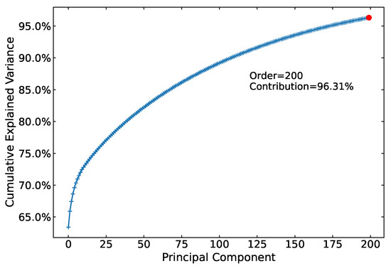
Figure 1.
Cumulative explained variance by principal component analysis (PCA) across different orders. The x-axis represents the principal component index, while the y-axis shows the cumulative explained variance percentage. A red dot highlights the contribution rate at order 200, achieving 96.31% cumulative variance explanation.
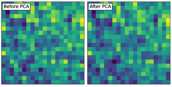
Figure 2.
Visual comparison of image reconstruction before and after principal component analysis (PCA). The left panel labeled “Before PCA” shows the original image, while the right panel labeled “After PCA” displays the reconstructed image using PCA. Both images are visually similar, indicating effective dimensionality reduction and reconstruction.
3. Method for Estimating Based on BP Neural Network
The concept of the BP network was proposed by Rinehart and McClelland et al. in 1986 [28]. Its topological structure includes an input layer, multiple hidden layers, and an output layer. The training process of the BP network consists of two parts: forward propagation and backward propagation. During forward propagation, the input signal passes through the hidden layer to the output nodes and undergoes non-linear transformations to generate the output signal. The error between the calculated forward propagation output and the given signal is then transferred to the backward propagation process. In this process, the error is recursively transmitted from the output nodes through the hidden layers, and the error is distributed to all units in each layer. The units obtain the error signal, which serves as the basis for weight adjustment. Through repeated learning and training, the network parameters corresponding to the minimum error are determined, and network training is completed.
The training process of BP neural network essentially adopts a global approximation method, which has good generalization ability and can be used as a general nonlinear input–output mapping model.
3.1. Design of Vision Estimation Algorithm Based on BP Neural Network
The correspondence between image and visual acuity is difficult to characterize using an analytical function. This multiple non-linear regression relationship can be established using the non-linear fitting ability of the BP neural network model. The input of the proposed BP-based visual acuity estimation network is a one-dimensional vector of size [1, 60] (preprocessed data), with a total of 8 hidden layers, and the output is a one-dimensional array of size [1, 1] (). The network uses the mean squared error () as the loss function, and the calculation formula is as follows:
In the hidden layer, ReLU (Rectified Linear Units) is used as the activation function [29]. In general, this function refers to the slope function in mathematics, which is given by the following:
The ReLU function is used as the activation function of a neuron, defining the non-linear output of the neuron after linear transformation . After using the activation function ReLU, for an input vector x from the previous neural network layer, its output is , which is then passed to the next layer of neurons or serves as the output of the entire network. Using the ReLU activation function has faster training speed, and networks with ReLU have performed better in some cases compared to those using other activation functions.
The initialization of network parameters uses random initialization. The learning rate is set as follows, with the initial learning rate of lr set to
During the training process, as long as the loss continues to decrease, the current learning rate remains unchanged. All data completed during training are recorded as one epoch. When the loss between two epochs decreases by less than or the validation score increases by less than , the learning rate is updated using the following equation:
Here, is the new learning rate. If the verification score in consecutive 10 epochs increases by less than , terminate training. To prevent the program from continuously training, the maximum number of iterations for training is set to 5000.
3.2. Algorithm Implementation Platform
The software environment of this algorithm is built using Python (Version 3.6.3) based on the Scikit-learn framework on Windows system. Scikit-learn (Version 0.24.2) is an open source, concise and efficient data mining and data analysis tool [30]. It includes commonly used modules for machine learning, making it easy to build your own network. The main information involved in the hardware environment of the algorithm is shown in Table 2:
Table 2.
Experimental environment.
4. Experimental Results and Discussion
When presenting the results of method testing, a 1:1 correlation line between predicted and actual values is used to present the training results of the network for evaluation. Take Figure 3 as an example, the horizontal axis represents the actual value, and the vertical axis represents the predicted value, with the mean square error of the training set and test set presented. This experiment mainly includes two parts: method testing and seeing change estimation for 22 consecutive years.
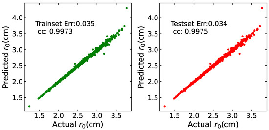
Figure 3.
Correlation diagram of training set and test set. The x-axis represents the actual values in centimeters, and the y-axis shows the predicted values. The training set plot, marked with green dots, has a mean squared error (MSE) of 0.035 and a correlation coefficient (cc) of 0.9973, indicating a high degree of accuracy and correlation. The test set plot, marked with red dots, has an MSE of 0.034 and a cc of 0.9975, also demonstrating a high level of accuracy and correlation.
4.1. Method Testing
The data obtained using the spectral ratio method were tested using this approach. Seventy percent (70%) of the data were selected as the training set, and thirty percent (30%) as the testing set. The experimental results are shown in Figure 3, where the horizontal and vertical axes represent the actual and predicted values, respectively (in units of cm). The mean square error of the training set and testing set is calculated using the following formula:
where represents the label value, and represents the predicted label value. From the experimental results, the mean square errors were 0.343 and 0.243, indicating that the data errors above were less than 0.68 cm and 0.48 cm, respectively. The correlation between the predicted and actual values was calculated using the following equation:
where and are the mean values of and , The correlation coefficients are 0.9973 and 0.9975. This result indicates that within a certain error range, this method can be used to estimate the of observed images. In the experiment, the error statistics of the test set were smaller than those of the training set, which may be due to the limited number of datasets.
4.2. Actual Estimation of from 1989 to 2010
Using the 22-year continuous solar photosphere image data accumulated at the HSOS from 1989 to 2010, we estimated the condition and calculated the median value for each year. The long-term seeing variation over the 22-year period is shown in Figure 4:
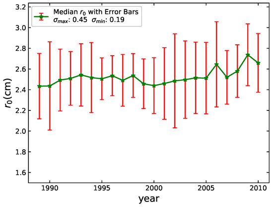
Figure 4.
Annual median change curve of value from 1989 to 2010. The x-axis represents the years, while the y-axis shows the median values in centimeters. Error bars indicate the maximum ( = 0.45) and minimum ( = 0.19) standard deviations.
The horizontal axis is the year, and the vertical axis is the value of . From the graph, the change in seeing is basically distributed between 2.5 and 3 cm, indicating that the seeing at the HSOS is stable within two solar activity cycles.
Take the median value of for each month of all years, and the curve of seeing variation from January to December is shown in Figure 5:
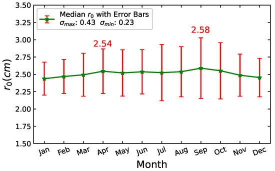
Figure 5.
Seeing change curve from January to December. The x-axis is months, and the y-axis is in cm. April and September have higher median values than adjacent months, as indicated by the green line and red error bars for standard deviations ( = 0.43 cm; = 0.23 cm).
The horizontal axis represents the months, ranging from January to December, while the vertical axis indicates the value in cm, ranging from 2.2 to 2.9 cm. The curve shows a general trend in seeing quality over the year. Here are the key observations from the graph: (i) starts at approximately 2.4 cm in January. (ii) There is an upward trend in seeing from January through April, reaching a peak around April. (iii) From May to August, seeing remains relatively stable with minor fluctuations. (iv) September sees the highest value of the year, marked at 2.58 cm. (v) A gradual decline in seeing is observed from September through December. Overall, the graph indicates the seasonal changes in seeing quality, with the best seeing occurring in September and the poorest in January and December. This pattern is consistent with practical observational experience, where atmospheric conditions often lead to variations in seeing quality throughout the year. The results reflect the typical influence of seasonal changes on atmospheric turbulence, which in turn affects astronomical seeing.
In Figure 6, we show the percentage of data where the seeing parameter is greater than 3 cm across all datasets.

Figure 6.
Percentage of greater than 3 cm from 1989 to 2010. The x-axis represents the years, ranging from 1989 to 2010, and the y-axis shows the percentage values. Each bar corresponds to a specific year and illustrates the proportion of exceeding 3 cm. Notable fluctuations are observed, with a significant peak in 2005, where the percentage reaches 22.7%.
The horizontal axis represents the year, and the vertical axis represents the percentage of cm. As can be seen from the figure, from 1989 year to 2010 year, almost every year, more than of the data were observed with an of greater than 3 cm. At most, of the data were observed with an greater than 3 cm. The results indicate that the seeing conditions were stable for a considerable proportion of the observation time period at the HSOS. The proportion of different sizes of in all data is shown in Figure 7. The majority of observations () were conducted under conditions where > 2 cm, with a significant decrease in percentage as increases. We can draw the following scientific conclusions: Firstly, atmospheric seeing at the observation site is generally favorable, with the vast majority of observations () completed under conditions where exceeded 2 cm. Secondly, while the majority of observations were conducted under relatively good conditions with greater than 2.5 cm, a significant proportion were also taken under extremely favorable atmospheric conditions. This suggests that the observing site occasionally experiences periods of very stable atmospheric conditions.
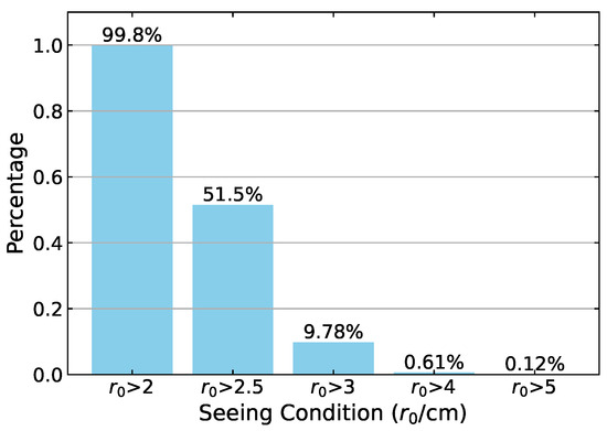
Figure 7.
Proportion of different sizes of . The x-axis represents the ranges ( > 2 cm, > 2.5 cm, > 3 cm, > 4 cm, > 5 cm), and the y-axis displays the corresponding percentage values. The majority of fall within the > 2 cm range, accounting for .
4.3. Systematic Error Estimation Experiment
The variations in seeing are consistent with the observational experience of our observers, as well as our conventional experience in data usage and interpretation. To further verify the effectiveness of the seeing estimation method proposed in this paper, we conducted actual tests at the HSOS. We compared the obtained from SDIMM and the spectral ratio method. SDIMM is an instrument specifically designed for measuring atmospheric , which calculates by observing the minute displacements at the edge of the Sun. The instrument uses a telescope with two sub-apertures, separated by an optical wedge prism on the focal plane to create two images of the solar edge, and it projects these images onto a CCD detector. By comparing the relative motion of these two images, the wavefront distortion caused by atmospheric turbulence can be calculated, thus obtaining the seeing parameter . SDIMM has the advantages of high-precision measurement, strong adaptability, high automation, and rich data, making it suitable for daytime observation, especially for measuring solar seeing.
This part of the experiment was conducted in cooperation with Southwest Jiaotong University and Yunnan Observatory, using the SDIMM they used for the CGST site selection at Wumingshan Mountain. This SDIMM is based on the previous research of Yunnan Observatory’s SDIMM. It is also equipped with independently developed calculation software, as shown in Figure 8.
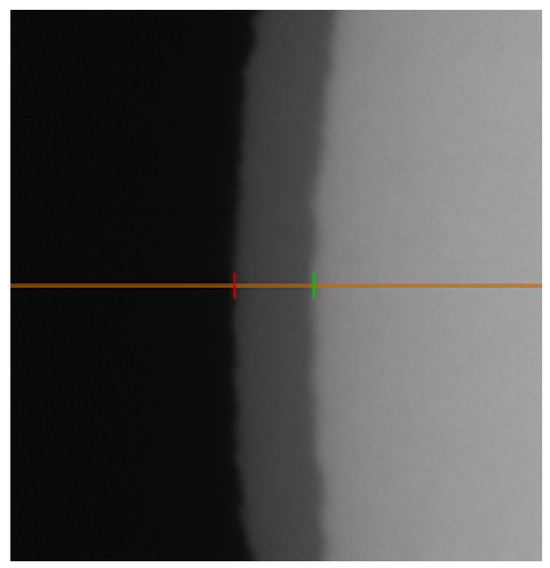
Figure 8.
Image observed by SDIMM System Software. The red and green lines represent the solar edges detected using the SDIMM software.
Through the tests conducted at Wuming Mountain, the effectiveness and reliability of the SDIMM in actual observation have been verified, providing important seeing data support for the CGST site selection. These test results not only verify the applicability of the SDIMM under different conditions but also provide actual observational data for comparison and reference for the seeing estimation method proposed in this paper. The specific parameters of the SDIMM are shown in Table 3:
Table 3.
Main parameters of SDIMM.
We conducted tests with and without a dome. The SDIMM is situated on a tripod approximately 2 m below the SMFT, as is shown in Figure 9.

Figure 9.
Comparative setup of the SDIMM under different observational conditions. The SMFT, represented by the larger white structure, is positioned above the SDIMM. (a) SDIMM deployed without a dome, showcasing the unobstructed exposure to the atmosphere, which is conducive to low-wind-speed and optimal seeing conditions. (b) SDIMM installed within the dome structure of the SMFT, designed to mitigate high-wind-speed and poor seeing conditions.
The calculation method of the SDIMM is as follows:
- The position of the solar limb is extracted using phase congruency algorithm, and the angle-of-arrival (AA) is calculated for a set of images. This part of the algorithm is detailed in the paper by Song et al. [7] and will not be repeated here;
- is calculated using the following formula:
where d represents the distance between the two sub-apertures, D denotes the diameter of the sub-aperture, and K is a constant related to the ratio of d to D [31]:
with .
The results are shown in Figure 10.
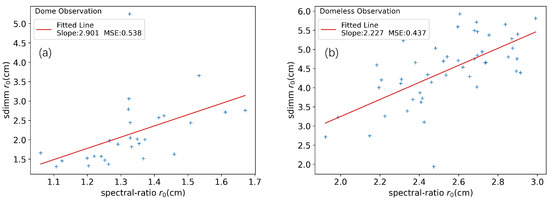
Figure 10.
The modulating effect of domes on seeing measurements under wind speed influence: (a) Dome observation results: shows the measurements taken during high wind speeds and poor seeing conditions. (b) Domeless observation results: presents the measurements taken during low wind speeds and good seeing conditions.
In this experiment, we compared the measured by the SDIMM and the spectral ratio method by averaging the results every minute, as shown in Figure 10. We also fitted the first-order coefficients of the SDIMM and spectral ratio method under conditions with and without a dome, and we calculated their mean square error (MSE). In domeless observation, the slope of the fitting line is 2.227, and the mean square error (MSE) is 0.437. In observation with a dome, the slope of the fitting line is 2.901, higher than in domeless observation, indicating that the relationship between the spectral ratio method and is more significant under dome conditions. The mean square error (MSE) is 0.538, slightly higher than in domeless observation, which may be due to increased atmospheric turbulence under high wind speeds. Although the MSE of dome observation is slightly higher, the steeper slope under high wind speeds indicates that the dome alleviates the negative impact of wind on measurement to some extent. This may be because the dome provides additional protection, reducing the direct impact of wind on atmospheric turbulence and thus stabilizing measurement.
If we consider the data obtained by SDIMM as the benchmark, the correlation between the measurements from SDIMM and the spectral ratio method, especially under domed conditions, demonstrates the consistently favorable seeing conditions at HSOS. The high fitting coefficients and low mean square errors (MSEs) further indicate that HSOS has excellent observational conditions, which are conducive to high-precision astronomical observations. This suggests that the site is exceptionally well suited for high-precision astronomical observations. Additionally, the results from other observation sites are shown in Table 4 [7,32]. Table 4 presents the median values for HOSO obtained by two different methods: one calculated using a neural network, and the other derived from spectral ratio analysis and SDIMM systematic error analysis. In the table, HSOS (neural network) indicates the results estimated from historical seeing data using the neural network proposed in this paper. HSOS (SDIMM) represents the values calculated by multiplying the HSOS (neural network) results by the slope shown in Figure 10b. As can be observed in the tabulated data, there are significant differences in the median values across different sites and periods, further highlighting the superior seeing conditions at HSOS among all the observation sites.
Table 4.
Comparison of median (cm) from several sites.
5. Summary and Outlook
This study addresses the challenge of assessing historical seeing data from available image data. It utilizes image data captured by existing observational instruments to train a neural network model. Furthermore, the paper introduces a novel neural-network-based approach for estimating long-term variations in seeing quality at astronomical observatories. Initially, we employ existing observational instruments to procure both single-frame and multi-frame short-exposure images. Subsequently, seeing parameter is derived for the composite images through the application of spectral ratio techniques. Ultimately, these data are amalgamated to form the dataset necessary for our analysis. We used PCA for dimensionality reduction during data preprocessing. Furthermore, a machine learning scheme based on the BP regression network is proposed. Then, the scheme was verified, and the results of seeing for 22 consecutive years were estimated. The method was fast and effective.
In the experiment of method testing, the dataset is randomly allocated as the training set and as the test set. From the experimental results, there is a strong correlation between the prediction results and label values of the training and testing sets. This method is effective for estimating the seeing using existing image data. The estimated results of the seeing stability for the 22 years from 1989 to 2010 show that the of the HSOS has been stable at around 2.5–3 cm for a long time. During all observation periods, the exceeded 3 cm for at least 2% of the time, and at its peak, it reached 22%. The correlation plot comparing SDIMM and spectral ratio methods shows that a dome significantly enhances the accuracy and stability of seeing measurements, especially under high wind speeds. Future research should delve deeper into the impact of dome design on seeing measurements and investigate how dome design can be optimized to adapt to a range of wind speed conditions.
This paper establishes a direct correspondence between images and seeing in a new way and machine learning methods, it and estimates the long-term seeing variations at astronomical observatories. This method can be used to estimate historical seeing at other sites in future applications.
Author Contributions
Conceptualization, X.H., S.Y. and X.B.; methodology, X.H. and S.Y.; software, X.H., S.Y. and T.S.; investigation, X.H. and S.Y.; resources, Y.D., T.S. and M.Z.; data curation, X.H. and S.Y.; writing—original draft preparation, X.H.; writing—review and editing, X.H., S.Y. and Y.L.; supervision, S.Y.; project administration, S.Y. and W.S.; funding acquisition, Y.D. and S.Y. All authors have read and agreed to the published version of the manuscript.
Funding
This research is supported by the National Key R&D Program of China No.2022YFF0503800, 2021YFA1600500, and 2022YFF0503001; National Natural Science Foundation of China (grants No. 12250005, 12073040, 12273059, 11973056, 12003051, 11573037, 12073041, 11427901, 11572005, 12373063 and 11611530679, 12473089, 12373057, and 62427804); the Strategic Priority Research Program of the China Academy of Sciences (grants No. XDB0560000, XDA15052200, XDB09040200, XDA15010700, XDB0560301, and XDA15320102); and the Chinese Meridian Project (CMP) and Yunnan Fundamental Research Projects (202401AT070140).
Data Availability Statement
The training and testing data, as well as parts of the workflow used in this study, are available online at https://gitee.com/steven-ux/seeing-estimation/tree/master/ (accessed on 23 April 2025). The dataset is available upon request from the authors.
Acknowledgments
We are grateful for the support of this project by the Specialized Research Fund for the State Key Laboratory of Solar Activity and Space Weather.
Conflicts of Interest
The authors declare no conflicts of interest.
References
- Fried, D.L. Optical Resolution Through a Randomly Inhomogeneous Medium for Very Long and Very Short Exposures. J. Opt. Soc. Am. 1966, 56, 1372–1379. [Google Scholar] [CrossRef]
- Liu, Z.; Qiu, P.Z.; Qiu, Y.H. Differential image motion visual acuity measurement experiment. Publ. Yunnan Obs. 1993, 4, 22–30. [Google Scholar]
- Deng, L.; Yang, F.; Chen, X.; He, F.; Liu, Q.; Zhang, B.; Zhang, C.; Wang, K.; Liu, N.; Ren, A.; et al. Lenghu on the Tibetan Plateau as an astronomical observing site. Nature 2021, 596, 353–356. [Google Scholar] [CrossRef] [PubMed]
- Liu, Z.; Deng, Y.Y.; Ji, H.S.; Li, H. Ground-based giant solar telescope of China. Sci. Sin. Phys. Mech. Astron. 2012, 12, 1282–1291. [Google Scholar] [CrossRef]
- Liu, Y.; Song, T.F.; Zhang, X.F.; Liu, S.; Zhao, M.; Tian, Z.; Miao, Y.; Li, H.; Huang, J.; Su, B.; et al. Progress of site survey for large solar telescopes in western China. Proc. Int. Astron. Union 2016, 11, 447–449. [Google Scholar] [CrossRef]
- Liu, Z.; Deng, Y.Y.; Yang, D.H.; Ji, H.S.; Jin, Z.Y.; Lin, J. Chinese Giant Solar Telescope. Sci. Sin. Phys. Mech. Astron. 2019, 49, 059604. [Google Scholar] [CrossRef]
- Song, T.F.; Wen, Y.M.; Liu, Y.; Elmhamdi, A.; Kordi, A.S.; Zhao, M.Y.; Zhang, X.F.; Li, X.B.; Wang, J.X.; Fu, Y.; et al. Automatic Solar Seeing Observations at Mt. Wumingshan in Western China. Sol. Phys. 2018, 2, 37. [Google Scholar] [CrossRef]
- Roggemann, M.C.; Welsh, B.M. Imaging Through Turbulence, 1st ed.; CRC Press: Boca Raton, FL, USA, 1996; pp. 154–196. [Google Scholar]
- Martin, H.M. Image Motion as a Measure of Seeing Quality. Publ. Astron. Soc. Pac. 1987, 99, 1360. [Google Scholar] [CrossRef]
- Liu, Z.; Lou, K.; Zhang, R.L.; Lu, R.W.; Beckers, J. The Day-time Seeing Monitor at Fuxian Lake and Some Primary Results. Publ. Yunnan Obs. 2000, 4, 95–100. [Google Scholar]
- Liu, Z.; Beckers, J.M. Comparative Solar Seeing and Scintillation Studies at the Fuxian Lake Solar Station. Sol. Phys. 2001, 198, 197–209. [Google Scholar]
- Wu, S.; Hu, X.D.; Han, Y.J.; Wu, X.; Su, C.; Luo, T.; Li, X. Measurement and analysis of atmospheric optical turbulence in Lhasa based on thermosonde. J. Atmos. Sol. Terr. Phys. 2020, 201, 105241. [Google Scholar] [CrossRef]
- Labeyrie, A. Attainment of Diffraction Limited Resolution in Large Telescopes by Fourier Analysing Speckle Patterns in Star Images. Astron. Astrophys. 1973, 6, 85–87. [Google Scholar]
- Deng, Y.Y.; Ai, G.X.; Zhang, B.; Qiu, P.Z.; Qiu, Y.H.; Liu, Z. High resolution image recovery in the region of the Sun. Sinica 1994, 35, 380–386. [Google Scholar]
- Krotov, D.; Hopfield, J. Large Associative Memory Problem in Neurobiology and Machine Learning. arXiv 2021, arXiv:2008.06996. [Google Scholar]
- Hinton, G.E.; Sejnowski, T.J. Optimal perceptual inference. In Proceedings of the IEEE Computer Society Conference on Computer Vision and Pattern Recognition, Washington, DC, USA, 19–23 June 1983; pp. 448–453. [Google Scholar]
- Hu, X.; Yang, S.B.; Ji, K.F.; Lin, J.B.; Deng, Y.Y.; Bai, X.Y.; Zhu, X.M.; Bai, Y.; Wang, Q. Calibration of Observing Wavelength Points of Birefringent Narrow Band Filter-Type Magnetograph Based on Neural Network. Chin. J. Lasers 2023, 13, 92–101. [Google Scholar]
- Huang, X.; Wang, H.N.; Xu, L.; Liu, J.; Li, R.; Dai, X. Deep Learning Based Solar Flare Forecasting Model. I. Results for Line-of-sight Magnetograms. Astrophys. J. 2018, 856, 11. [Google Scholar] [CrossRef]
- Yuan, Y.; Shih, F.; Jing, J.; Wang, H. Automated flare forecasting using a statistical learning technique. Res. Astron. Astrophys. 2010, 10, 785–796. [Google Scholar] [CrossRef]
- Hu, T.Z.; Zhang, Y.; Cui, X.Q.; Zhang, Q.Y.; Li, Y.P.; Cao, Z.H.; Pan, X.S.; Fu, Y. Telescope performance real-time monitoring based on machine learning. Mon. Not. R. Astron. Soc. 2012, 1, 388–396. [Google Scholar] [CrossRef]
- Guo, J.J.; Bai, X.Y.; Deng, Y.Y.; Liu, H.; Lin, J.B.; Su, J.T.; Yang, X.; Ji, K.F. A Non-Linear Magnetic Field Calibration Method for Filter-Based Magnetographs by Multilayer Perceptron. Solar Phys. 2020, 295, 18. [Google Scholar] [CrossRef]
- Wen, X.; Li, X.; Zhang, X.W. Implementing Neural Networks with MATLAB, 1st ed.; National Defence Industry Press: Beijing, China, 2015; pp. 95–100. [Google Scholar]
- Mitchell, T.M. Machine Learning, 1st ed.; International Edition: New York, NY, USA, 1997; pp. 9–20. [Google Scholar]
- Haykin, S.O. Neural Networks and Learning Machines, 1st ed.; Pearson: New York, NY, USA, 2008; pp. 15–25. [Google Scholar]
- Wang, J.M.; Qian, Z.Y.; Ai, G.X.; Shi, Z.X.; Hu, Y.F. Comparison of candidate solar optical observation sites in Shahe, Xinglong, and Huairou (II)—Observation of atmospheric temperature fluctuations in the near surface layer. Acta Astron. Sin. 1977, 02, 182–191. [Google Scholar]
- Ai, G.X.; Li, W.; Zhang, H.Q. FeI lambda 5324.19 A line forms in the solar magnetic field and the theoretical calibration of the solar magnetic field telescope. Acta Astron. Sin. 1982, 23, 39–48. [Google Scholar]
- von der Lühe, O. Estimating Fried’s parameter from a time series of an arbitrary resolved object imaged through atmospheric turbulence. J. Opt. Soc. Am. 1984, 5, 510–519. [Google Scholar] [CrossRef]
- Rumelhart, D.E.; Hinton, G.E.; Williams, R.J. Learning representations by back-propagating errors. Nature 1986, 323, 533–536. [Google Scholar] [CrossRef]
- Nair, V.; Hinton, G.E. Rectified linear units improve restricted Boltzmann machines. In Proceedings of the 27th International Conference on Machine Learning, Haifa, Israel, 21–24 June 2010. [Google Scholar]
- Guido, S.; Mueller, A.C. Introduction to Machine Learning with Python, 1st ed.; O’Reilly Media: New York, NY, USA, 2016; pp. 154–166. [Google Scholar]
- Tokovinin, A. From Differential Image Motion to Seeing. Publ. Astron. Soc. Pac. 2002, 114, 1556–1566. [Google Scholar] [CrossRef]
- Özışık, T.; Ak, T. First day-time seeing observations at the TÜBİTAK. Astron. Astrophys. 2004, 3, 1129–1133. [Google Scholar] [CrossRef]
Disclaimer/Publisher’s Note: The statements, opinions and data contained in all publications are solely those of the individual author(s) and contributor(s) and not of MDPI and/or the editor(s). MDPI and/or the editor(s) disclaim responsibility for any injury to people or property resulting from any ideas, methods, instructions or products referred to in the content. |
© 2025 by the authors. Licensee MDPI, Basel, Switzerland. This article is an open access article distributed under the terms and conditions of the Creative Commons Attribution (CC BY) license (https://creativecommons.org/licenses/by/4.0/).