Dust Universes in Higher Dimensions with Gauss–Bonnet Corrections

Abstract

We study dust models in higher-dimensional general relativity and the Einstein–Gauss–Bonnet theory in a maximally symmetric spacetime. We show that the dynamics of the model is governed by an Abel differential equation of the second kind. This equation is solved in general for all arbitrary dimensions and spatial curvature to yield solutions for the cosmic scale factor. We show that the existence of the first integral determining the dynamics of dust can be demonstrated without additional assumptions. Analysis of the first integral shows that explicit and implicit solutions are possible depending on the presence of the cosmological constant. Comparisons between the higher-order theory and general relativity are discussed in detail.

1. Introduction

Dust models have been studied over the years in various gravity theories. These are exact solutions of the field equations that have positive energy density; however, the distribution of matter in question has vanishing pressure. They represent highly idealised representations of clusters of galaxies, and they serve as a first approximation for studying galactic dynamics. Dust models also provide simple frameworks to study gravitational collapse in relativistic astrophysics. Many interesting physical features arise in studies within general relativity, and these are reflected in the reviews by Harrison [1], Vajk [2], and Stephani et al. [3]. A comprehensive study of charged dust matter distributions in spherically symmetric fields incorporating general relativistic effects was undertaken by Raychaudhuri [4]. Clearly, if the pressure is nonvanishing then we obtain the standard Friedmann–Lemaître–Robertson–Walker (FLRW) cosmological models, usually with a barotropic equation of state [5]. The survey of generalised FLRW models by Mantica and Molinari [6] shows that these models may be extended to include effects of spatial inhomogeneity. The dynamics of the universe was discussed in [7,8], where a solution for the scale factor was provided for the general linear equation of state via an alternative approach, first introduced by [5], where, instead of using physical cosmic time, a conformal time parameter was introduced, and the general equations of motion were then derived. It was then shown that for the spatially flat universe, the system behaves like a free particle. For the closed, spherical universe, the system behaves like a simple harmonic oscillator for any value of the equation-of-state parameter. For the open, hyperbolic universe, the system acts like an anti-oscillator: a particle that is subjected to a repulsive force which is proportional to the distance.

Lovelock gravity theories have been studied extensively in recent decades. They allow for higher-dimensional interactions that reduce to general relativity as the low-energy effect theory. They represent models of gravity that contain field equations with second-order derivatives of the metric tensor but the action functional can be a higher-degree polynomial involving the curvature tensor. For quadratic polynomials we obtain the Einstein–Gauss–Bonnet (EGB) action, which has been comprehensively studied because of consistency involving the expanding universe, its astrophysical applications, and its relations to string theory. For some recent treatments in this direction, see the papers of Rej et al. [9], Chatterjee and Jaryal [10], and Maurya et al. [11]. There have been some attempts to study charged static dust spheres in EGB gravity. The first exact dust solution in a static spherically symmetric geometry, in EGB gravity, was found by Hansraj [12] in closed form in $N=5$ and $N=6$ dimensions. A wider class of exact solutions, with the same geometry, was obtained by Naicker et al. [13] for arbitrary N; in this treatment it is shown that the dynamical behaviour of the dust model is governed by an Abel differential equation, which is different from general relativity. The results of [13] contain the solutions of [12] as a special case. The collapse of an inhomogeneous dust was also analysed in five-dimensional EGB gravity in [14], where Tolman–Lemaître–Bondi-type spacetime was discussed with the addition of the higher-order Gauss–Bonnet terms. A timelike and weak singularity formed as a consequence of collapse, which is forbidden in general relativity, showing that the effects of the Gauss–Bonnet corrections can vastly affect the overall dynamics of a physical system. Several other applications of the EGB theory with regards to gravitational collapse and black holes were conducted in [15,16,17,18,19,20]. We note that there are several reasons for increasing dimensions and modifying general relativity to include higher-order curvature terms. Firstly, general relativity is a global physical theory and does not explain physics on very large (or very small) scales, due to the fact that it is not well tested in those extremes. Examples include the accelerated late-time expansion of the universe, as well as dark energy and dark matter, on large scales, and the singularity problem of black holes on infinitely small scales. In addition to appearing in the low-energy limit of heterotic string theory, the presence of the higher-order curvature terms of the EGB theory, as well as the extra dimensions, could perhaps explain dark matter and dark energy and this accelerated expansion. We show that the presence of the higher-order terms, in tandem with the cosmological constant, which is vacuum energy, increases the rate of cosmic expansion, and thus these higher-order terms may be a good candidate, collectively, for accelerated expansion.

Cosmology in modified gravity has been the subject of in depth analysis by several authors. For example, some analytical solutions were found in $f\left(T\right)$ gravity for a maximally symmetric spacetime containing a dust fluid and radiation as well as for an empty anisotropic Bianchi I universe in [21]. A dynamical systems analysis was conducted for the non-flat universe in the context of $f\left(Q\right)$ gravity, a non-metric theory, in [22]. Within the $f\left(R\right)$ modification, which includes fourth-order equations of motion, as well as scalar fields, some cosmological solutions were found and analysed in [23,24,25,26,27]. As far as we are aware, expanding dust models in EGB gravity have not been well studied. Cosmological solutions in the Lovelock theory were obtained by Deruelle and Fariña-Busto [28] for FLRW spacetimes, maximally symmetric spacetimes and indeed product manifolds of symmetric subspaces—that is, the product of an external FLRW spacetime and an internal maximally symmetric compact space. Cosmic inflation as well as late-time acceleration within the framework of quantum Lovelock gravity was analysed by Bousder et al. [29,30]. The inflationary model was discussed in the context of the Lovelock theory in [31] and the exact transition amplitude for EGB gravity with Neumann/Robin boundary conditions was analysed in a review in [32]. A recent treatment in general Lovelock theory attempts to describe various expanding dust-type models in the context of higher dimensions and orders [33]. However, the resulting solutions depend on solving a higher-order polynomial equation, a difficult endeavour. The novelty of our approach is that we can integrate the resulting dynamical cosmological equation in EGB gravity, in general, to obtain a first integral; explicit and implicit forms of the scale factor are obtained. In this paper, we demonstrate that expanding dust solutions are possible in EGB theories within a higher-dimensional FLRW geometry. Interestingly, the matter distribution in expanding dust models is neutral, which is in contrast to static models, which are necessarily charged. We solve the EGB field equations and also regain (and extend) solutions in higher-dimensional general relativity.

2. The Expanding Universe

The dynamics of the gravitational field can be extended to higher dimensions in an elegant generalisation of classical general relativity by including higher-order curvature corrections in EGB gravity. EGB gravity is contained within the Lovelock class of theories. This is characterised by field equations which contain second-order derivatives of the metric tensor and an additional term in the standard Einstein–Hilbert action, which is quadratic in the Riemann tensor. The EGB field equations are given by

$$G_{ab}-{\displaystyle \frac{\alpha }{2}}{H}_{ab}+\mathrm{\Lambda }{g}_{ab}={\kappa }_N{T}_{ab}.$$

(1)

where $\mathrm{\Lambda }$ is the cosmological constant, $\alpha$ is the EGB coupling constant, and the tensor $H_{ab}$ is the second-order Lovelock tensor; this contains higher-order curvature corrections. Einstein’s coupling constant in higher dimensions is given in terms of the Gamma function as

$${\kappa }_N={\displaystyle \frac{2(N-2){\pi }^{\frac{N-1}{2}}}{(N-3)\mathrm{\Gamma }\left(\frac{N-1}{2}\right)}}.$$

The Lovelock tensor allows for great insight into the geometric nature of gravity and is described by

$$H_{ab}=g_{ab}{L}_{GB}-4R{R}_{ab}+8R_{ac}{R^c}_b+8R^{cd}{R}_{acbd}-4{R_a}^{cde}{R}_{bcde}.$$

(2)

The quantity $L_{GB}$ is the Lovelock term that is quadratic in the Riemann tensor, Ricci tensor, and the Ricci scalar, and has the specific form

$$L_{GB}=R^2+R_{abcd}{R}^{abcd}-4R_{cd}{R}^{cd}.$$

(3)

The Lovelock tensor vanishes identically when $N<5$; the above term $L_{GB}$ is merely a geometrical invariant in four dimensions but vanishes for $N<4$. Ultimately, the law of conservation necessitates that

$${H^{ab}}_{;b}=0,$$

(4)

in addition to the second-differential Bianchi identities. When $\alpha =0$ in (1), we obtain higher-dimensional general relativity. The presence of the Lovelock tensor leads to greater complexity in the field equations in modified gravity theories, as discussed in Padmanabhan and Kothawala [34] and Shankaranarayan and Johnson [35]. The dynamics of matter change in higher dimensions, as emphasised by Zwiebach [36] in a study involving the connection between string theory and cosmology.

It is possible to extend the standard homogeneous and isotropic geometry from four to higher dimensions, so that the FLRW metric in N dimensions is given by

$$\begin{array}{ccc}\hfill d{s}^2& =& -d{t}^2+{\left({\displaystyle \frac{a\left(t\right)}{1+k{r}^2}}\right)}^2\left(d{r}^2+r^{2}d{\mathrm{\Omega }}_{N-2}^2\right).\hfill \end{array}$$

(5)

where $k=0,-1,+1$ represents the spatial curvature and $a\left(t\right)$ is the scale factor. The metric for the unit-$(N-2)$ sphere has the form

$$\begin{array}{ccc}\hfill d{\mathrm{\Omega }}_{N-2}^2& =& \sum _{i=1}^{N-2}\left(\left[\prod _{j=1}^{i-1}\left({sin}^2{\theta }_j\right)\right]{\left(d{\theta }_i\right)}^2\right).\hfill \end{array}$$

(6)

This result is kinematical and holds in any theory of gravity for maximally symmetric spacetimes. The theory of gravity selected determines the profile of the scale factor $a\left(t\right)$.

The assumption of an exactly homogeneous and isotropic universe yields a maximally symmetric manifold in N dimensions. The higher-dimensional EGB field equations are given as

$$\begin{array}{ccc}\hfill {\kappa }_N\rho & =& {\displaystyle \frac{(N-1)(N-2)}{2a^2}}({\dot{a}}^2+4k)\left[1+{\displaystyle \frac{\widehat{\alpha }}{a^2}}({\dot{a}}^2+4k)\right]-\mathrm{\Lambda },\hfill \\ \hfill {\kappa }_{N}p& =& -{\displaystyle \frac{(N-2)}{a}}\left(\ddot{a}+{\displaystyle \frac{N-3}{2a}}({\dot{a}}^2+4k)\right)\hfill \end{array}$$

(7a)

$$\begin{array}{ccc}& & -{\displaystyle \frac{2(N-2)\widehat{\alpha }}{a^3}}({\dot{a}}^2+4k)\left[\ddot{a}+{\displaystyle \frac{N-5}{4a}}({\dot{a}}^2+4k)\right]+\mathrm{\Lambda },\hfill \end{array}$$

(7b)

where we have set $\widehat{\alpha }=\alpha (N-3)(N-4)$ for convenience. We have included the cosmological constant $\mathrm{\Lambda }$.

The higher-dimensional energy conservation equation ${T^{ab}}_{;b}=0$ is

$$\dot{\rho }+(N-1){\displaystyle \frac{\dot{a}}{a}}(\rho +p)=0.$$

(8)

The condition (8) can equivalently be derived from the field Equation (7). When we set $\alpha =0$ and $N=4$, we regain ipso facto original general relativity. From this, we can establish that a nonvanishing Gauss–Bonnet invariant $\alpha \ne 0$ has an evident effect on the dynamics of the spacetime. However, a special case arises when $N=5$ since the term ${\displaystyle \frac{N-5}{4a}}({\dot{a}}^2+4k)$ vanishes, and we can therefore discern that the dynamics is inherently different from $N\ge 6$. It is thus essential that all values of N should be considered when $\alpha \ne 0$. The cosmic dynamics of the universe can be determined via a combination of the two field equations, either in the form of an equation of state or via another assumption like cosmic dust with $p=0$.

If we consider (7a) with $\mathrm{\Lambda }=0$, it can be written as

$$\widehat{\alpha }{H}^4+\left(1+{\displaystyle \frac{\widehat{\alpha }}{a}}k\right)H^2={\displaystyle \frac{2{\kappa }_N\rho }{(N-1)(N-2)}}-{\displaystyle \frac{4k}{a}}\left(1+4\widehat{\alpha }k\right),$$

(9)

in terms of the Hubble parameter

$$H={\displaystyle \frac{\dot{a}}{a}}.$$

The Hubble parameter is time-dependent, whereas the Hubble constant $H_0$ is a measure of the said parameter at any instant of cosmological time. Often in the literature, both terminologies are used interchangeably, which is incorrect. Equation (9) is the EGB generalisation of the Friedmann equation. In N-dimensional general relativity, this reduces to

$$H^2={\displaystyle \frac{2{\kappa }_N\rho }{(N-1)(N-2)}}-{\displaystyle \frac{4k}{a}}.$$

(10)

Equations (9) and (10) are alternative ways to represent the generalised Friedmann equation in terms of the Hubble parameter, in EGB gravity and in higher-dimensional general relativity, respectively.

3. Dust Models in N-Dimensional General Relativity

In astrophysics, dust models are studied as a consequence of their application to stars, galactic dynamics, accretion discs, and quasars. A recent investigation along these lines is given by Garcia-Reves [37] for conformastatic dust disks. Therefore, a special case that is physically important arises in the pressure-free distribution. In general relativity, the higher-dimensional Einstein field equations are

$$\begin{array}{ccc}\hfill {\kappa }_N\rho & =& {\displaystyle \frac{(N-1)(N-2)}{2a^2}}({\dot{a}}^2+4k)-\mathrm{\Lambda },\hfill \end{array}$$

(11a)

$$\begin{array}{ccc}\hfill {\kappa }_{N}p& =& -{\displaystyle \frac{(N-2)}{a}}\left(\ddot{a}+{\displaystyle \frac{N-3}{2a}}({\dot{a}}^2+4k)\right)+\mathrm{\Lambda },\hfill \end{array}$$

(11b)

where the dimension N is explicit. If we set

$$p=0,z={\dot{a}}^2+4k,$$

in Equation (11b), we arrive at the cosmic dust equation,

$${\displaystyle \frac{1}{2}}{a}^2{\displaystyle \frac{dz}{da}}+{\displaystyle \frac{1}{2}}(N-3)az-{\displaystyle \frac{\mathrm{\Lambda }{a}^3}{N-2}}=0,$$

(12)

which is a linear differential equation in z.

Therefore, the general solution to Equation (12) can be obtained, after some calculation, as

$$a^{N-3}z-{\displaystyle \frac{2\mathrm{\Lambda }{a}^{N-1}}{(N-1)(N-2)}}=a_0,$$

(13)

where $a_0$ is an integration constant. The above solution for z is the first integral for $a\left(t\right)$. We now consider two separate cases.

3.1. Case I: $\mathrm{\Lambda }=0$, $a_0\ne 0$

When $\mathrm{\Lambda }=0$, the first integral (13) becomes

$$z={\displaystyle \frac{a_0}{a^{N-3}}}.$$

(14)

Usually, on physical grounds, this constant is set to zero. The scale factor is initially zero at the beginning of all cosmic time, or the birth of the universe, which is why the constant of the first integral is usually taken to vanish. However, we can write

$${\dot{a}}^2={\displaystyle \frac{a_0}{a^{N-3}}}-4k,$$

(15)

which is a generalisation to higher dimensions of the result obtained by Lima [8]. The above equation can also be written in terms of the Hubble parameter as

$$H^2={\displaystyle \frac{a_0}{a^{N-1}}}-{\displaystyle \frac{4k}{a^2}},H={\displaystyle \frac{\dot{a}}{a}}.$$

(16)

We note that if a spatially flat universe $(k=0)$ is assumed, Equation (15) then admits an explicit general solution. This solution is given by

$$a\left(t\right)={\left[a_0\left({\displaystyle \frac{N-1}{2}}\right)(t+a_1)\right]}^{{\displaystyle \frac{2}{N-1}}}.$$

(17)

where $a_1$ is a second integration constant and $a_0>0.$ The effects of the spacetime dimension N are explicit in the evolution of the cosmic scale factor. We also make the note that from (17), the derivative $\dot{a}\left(t\right)>0$ for all dimensions, which indicates an expanding universe; this is not surprising. The second derivative $\ddot{a}\left(t\right)<0$ for all dimensions, which indicates that the expansion of the spatially flat universe is decelerating over time. In the four dimensional scenario, (17) reduces to

$$a\left(t\right)=a_0{\left({\displaystyle \frac{3}{2}}\right)}^{{\displaystyle \frac{2}{3}}}{(t+a_1)}^{{\displaystyle \frac{2}{3}}},$$

(18)

which was obtained by Lima [8].

If the universe is curved in any spatial manner, id est $k=1,-1$, the solution to (15) can be given implicitly in terms of hypergeometric functions as

$${\displaystyle \frac{a{\sqrt{1-\frac{a_0{a}^{N-3}}{4k}}}_2{F}_1\left(\frac{1}{2},\frac{1}{3-N};1+\frac{1}{3-N};\frac{a_0{a}^{N-3}}{4k}\right)}{\sqrt{a_0{a}^{N-3}-4k}}}=t+a_1.$$

(19)

If the dimension is specified, some progress can be made in obtaining a simpler closed-form solution. For example, when $N=4$, the solution is implicit in nature and is given by

$$-{\displaystyle \frac{1}{8k^{\frac{3}{2}}}}\left[a_1{tan}^{-1}\left({\displaystyle \frac{1}{2\sqrt{k}}}\sqrt{{\displaystyle \frac{a_0}{a}}-4k}\right)-2\sqrt{k}a\sqrt{{\displaystyle \frac{a_0}{a}}-4k}\right]=t+a_1,$$

(20)

where $k\ne -1$. If the dimension of spacetime is $N=5$, the solution is remarkably then an explicit closed-form one given, for the two additional values of the spatial curvature k, by

$$a\left(t\right)=\left\{\begin{array}{cc}\sqrt{2a_0(t+a_1)},\hfill & k=0\hfill \\ {\displaystyle \frac{1}{2}}\sqrt{-a_0-16{(a_1-t)}^2},\hfill & k=1\hfill \\ {\displaystyle \frac{1}{2}}\sqrt{16(t+a_1)-a_0},\hfill & k=-1\hfill \end{array}\right.$$

It is important to note that the $N=5$ scenario is the only such one where a closed-form explicit solution for the scale factor can be obtained for $k=\pm 1$. We note that a closed universe $k=1$ is not possible in five dimensions since we have that $a_0<0$, which contradicts (16). For all dimensions where $N>5$, the solution for the scale factor is obtained in terms of special functions, namely, hypergeometric functions—the four-dimensional universe is also distinct since the implicit solution (20) can be obtained in that case. 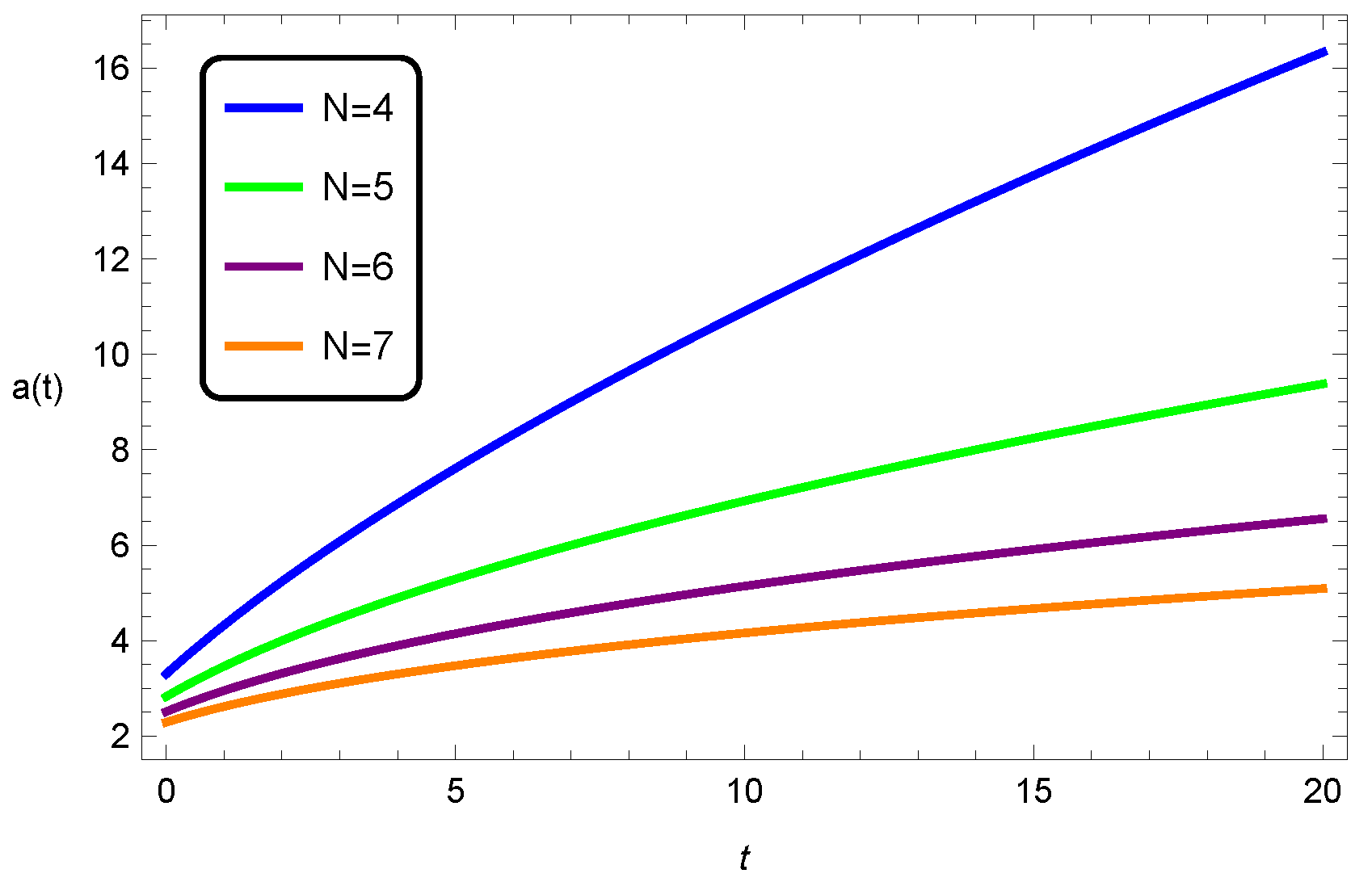In Figure 1, we see the evolution of the scale factor (17) for several dimensions in the universe of flat spatial curvature; an increase in dimension appears to slow the scale factor’s evolution. 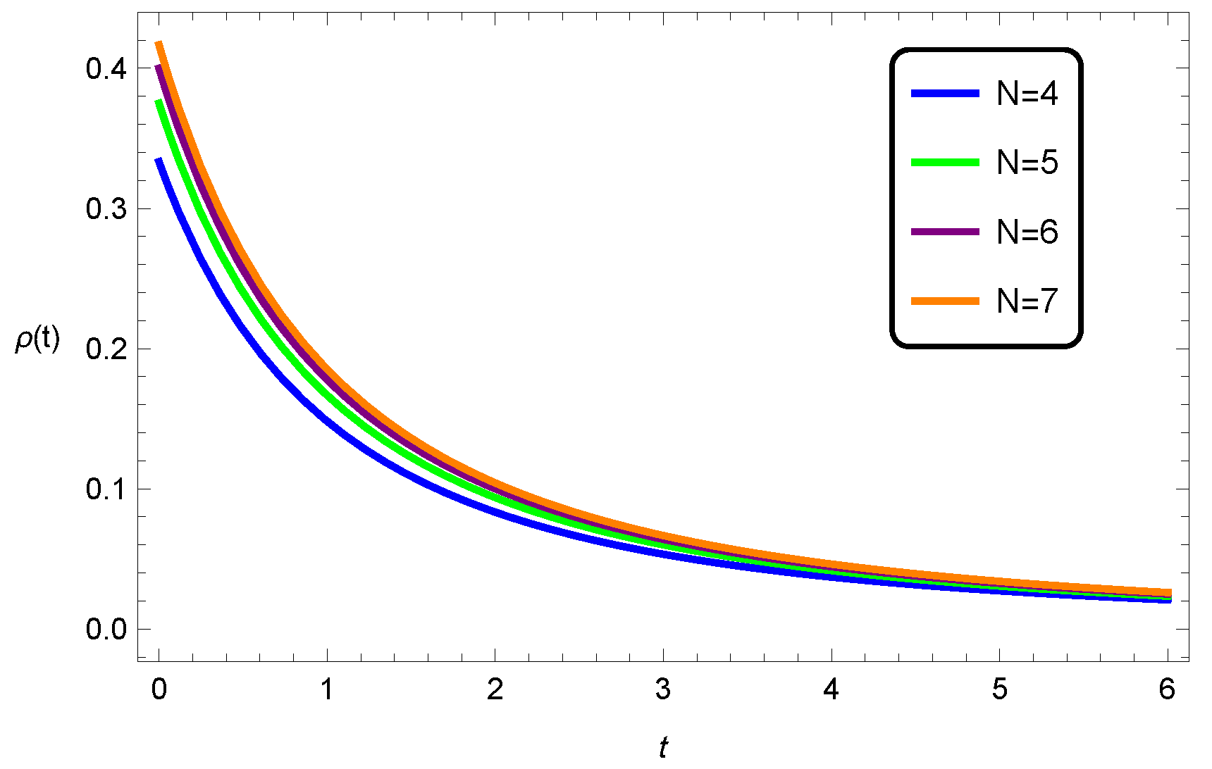Figure 2 depicts the behaviour of the energy density for several dimensions, with the solution (17). The energy density is everywhere positive and well defined and decreases over time, with the behaviour appearing similar for all dimensions.

3.2. Case II: $\mathrm{\Lambda }\ne 0$, $a_0=0$

In the case of a nonvanishing cosmological constant and $a_0=0$, Equation (13) reduces to the following:

$$z={\displaystyle \frac{2\mathrm{\Lambda }{a}^2}{(N-1)(N-2)}}.$$

(21)

Since ${\dot{a}}^2=z-4k$, we can write

$$\dot{a}=\sqrt{{\displaystyle \frac{2\mathrm{\Lambda }}{(N-1)(N-2)}}{a}^2-4k}.$$

(22)

This equation is a separable differential equation and, depending on the value of the spatial curvature k, can be solved to yield

$$a\left(t\right)=\left\{\begin{array}{cc}{a}_{1}exp\left[\sqrt{{\displaystyle \frac{2\mathrm{\Lambda }}{(N-1)(N-2)}}}t\right],\hfill & k=0\hfill \\ \sqrt{{\displaystyle \frac{2(N-1)(N-2)}{\mathrm{\Lambda }}}}cosh\left[\sqrt{{\displaystyle \frac{2\mathrm{\Lambda }}{(N-1)(N-2)}}}(t+a_1)\right],\hfill & k=1\hfill \\ \sqrt{{\displaystyle \frac{2(N-1)(N-2)}{\mathrm{\Lambda }}}}sinh\left[\sqrt{{\displaystyle \frac{2\mathrm{\Lambda }}{(N-1)(N-2)}}}(t+a_1)\right],\hfill & k=-1\hfill \end{array}\right.$$

which is in terms of exponential and hyperbolic trigonometric functions, as well as the dimension N. From the above, we can see that $\mathrm{\Lambda }>0$, thus an anti-de Sitter type universe is not possible. We also note that the presence of the cosmological constant term generates a physical solution for the closed universe $k=1$, for all dimensions, unlike the five-dimensional case mentioned previously for nonvanishing $a_0$. For any spatial curvature $k=0,\pm 1$, the derivative $\dot{a}\left(t\right)>0$ for all cosmological time, which again indicates an expanding universe for all $N\ge 4$. This is unsurprising as the solutions for all spatial curvatures are exponential in nature. We also have that $\ddot{a}\left(t\right)>0$, which indicates an accelerated expansion, thus the presence of the cosmological constant term has a direct effect on the expansion of either the flat, open, or closed universe; the de Sitter universe is expanding at an accelerating rate.

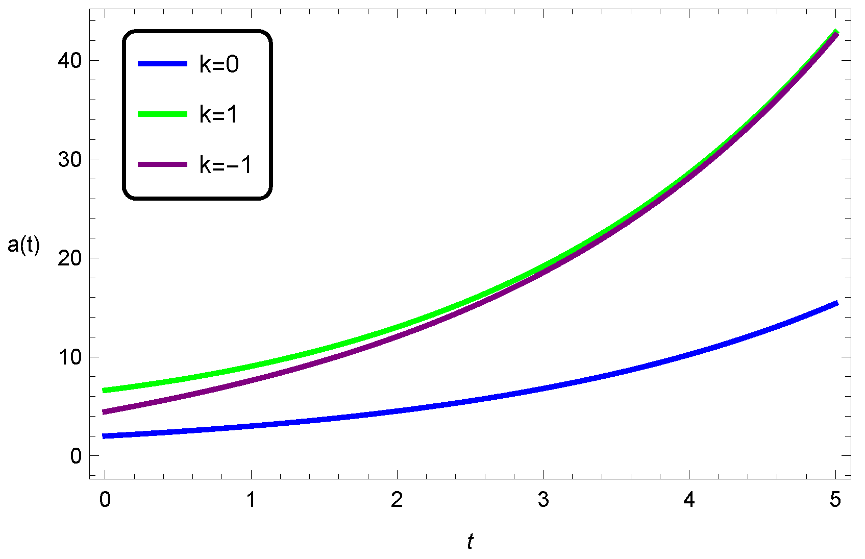
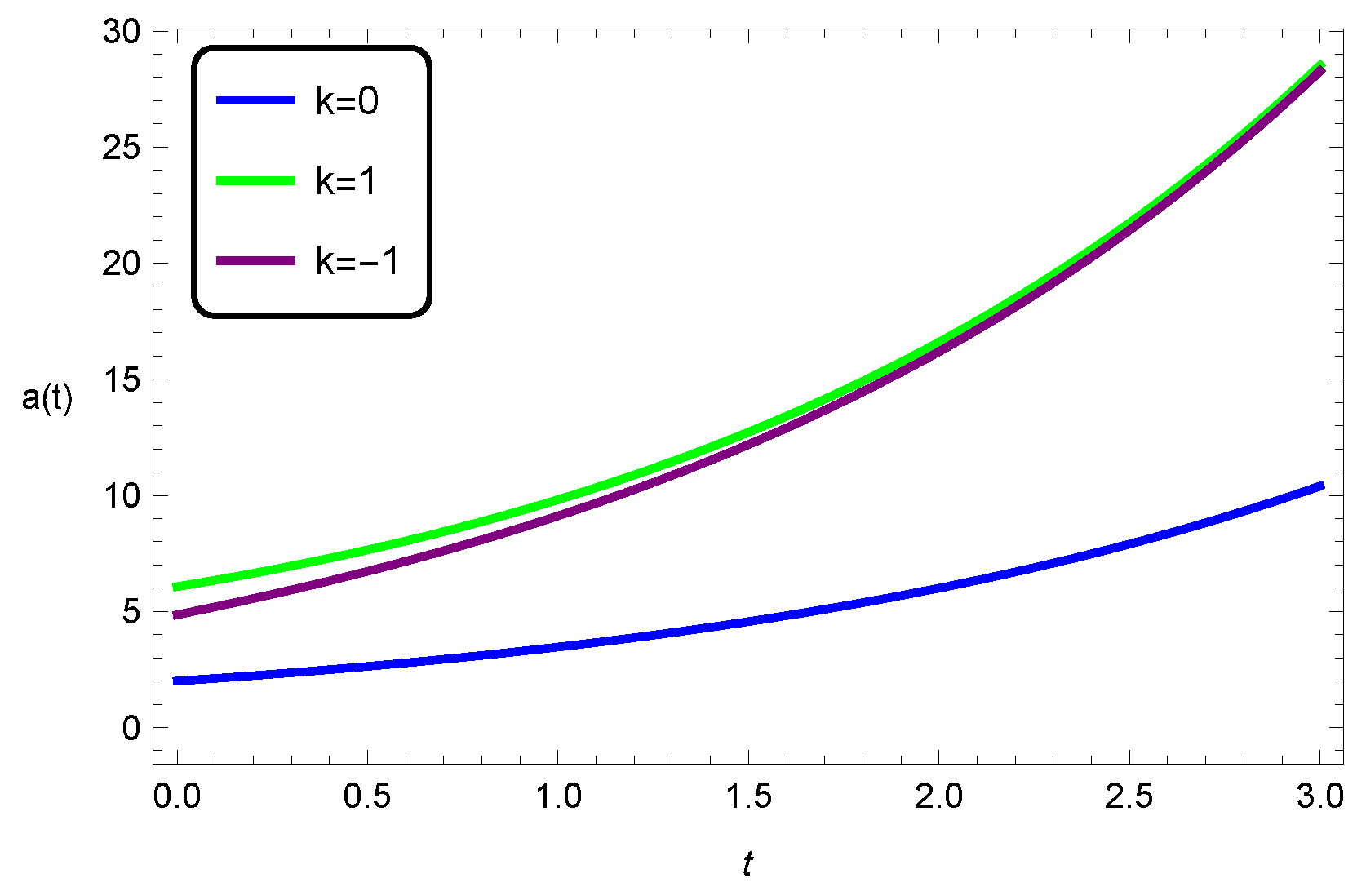
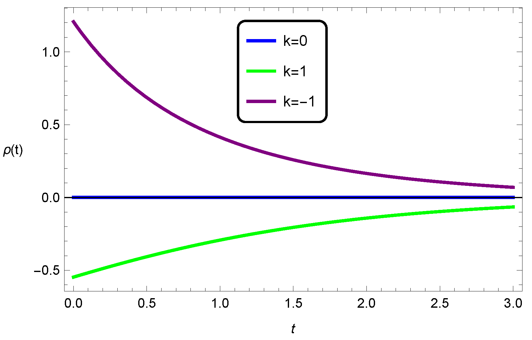
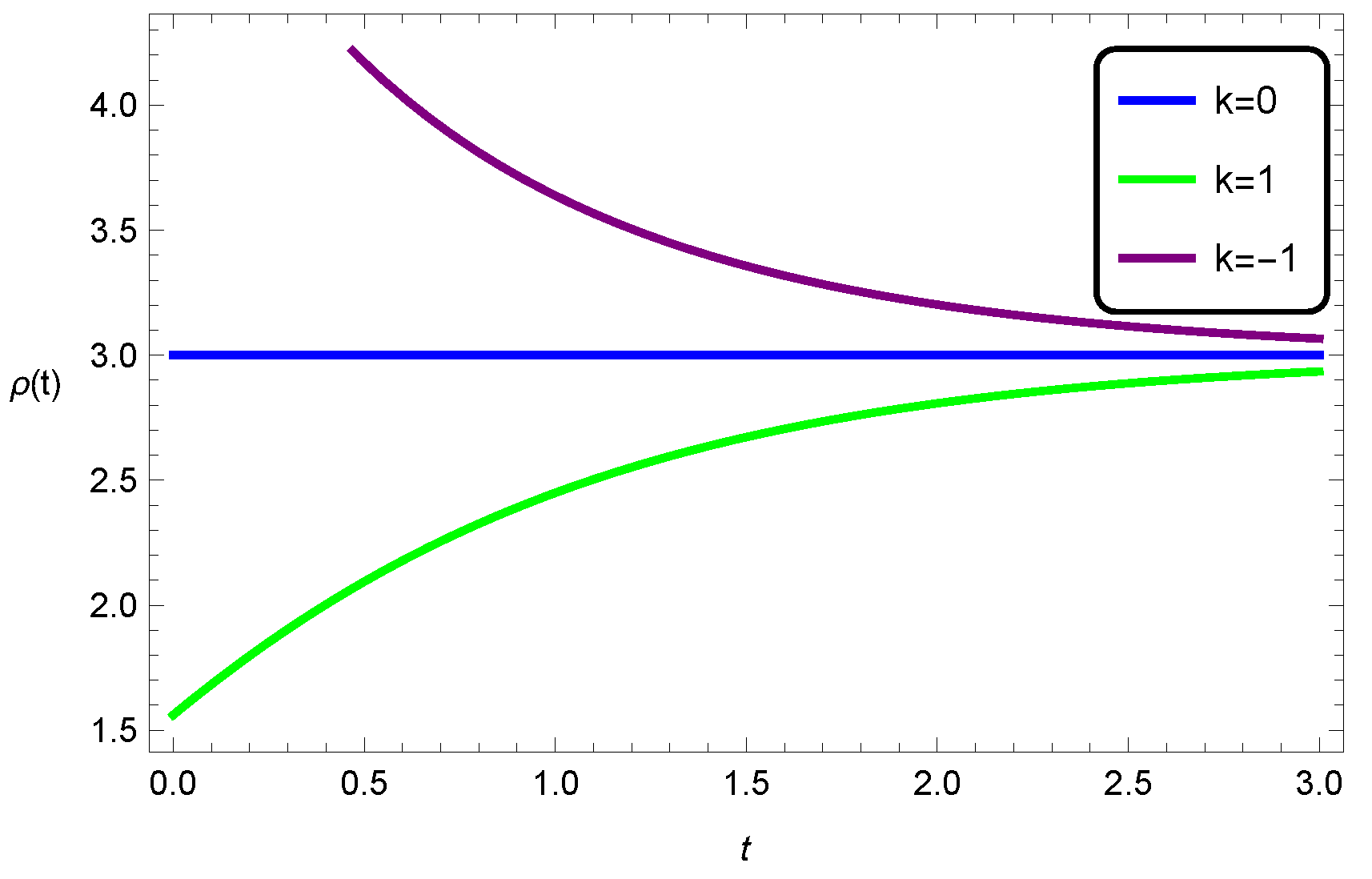
Figure 3 depicts the behaviour of the scale factor for all spatial curvatures for a nonvanishing and positive cosmological constant. All three cases depict increasing behaviour; however, the rate of increase is higher for the open and closed de Sitter universes. Figure 4 depicts the behaviour of the energy density for all spatial curvatures in five dimensions. We can see that in the flat universe the energy density $\rho =0$, and for the closed universe, the energy density is always negative, which is an unacceptable notion. However, for the open universe the situation is corrected and the energy density is positive and decreasing over cosmic time. We note that these plots were created for the five-dimensional scenario so that comparisons with the physics of the EGB universe is then a possibility.

4. Dust Models in Higher-Dimensional EGB Gravity

The dynamics of the dust model are greatly influenced by the higher-order curvature corrections indicative of EGB gravity. Analogously, if we set

$$p=0,z={\dot{a}}^2+4k,$$

in system (7), we then obtain

$$\begin{array}{ccc}\hfill {\kappa }_N\rho & =& {\displaystyle \frac{(N-1)(N-2)}{2a^2}}z\left[1+{\displaystyle \frac{\widehat{\alpha }}{a^2}}{z}^2\right]-\mathrm{\Lambda },\hfill \end{array}$$

(23a)

$$\begin{array}{ccc}\hfill 0& =& \left({\displaystyle \frac{1}{2}}{a}^2+\widehat{\alpha }z\right){\displaystyle \frac{dz}{da}}+{\displaystyle \frac{1}{2}}(N-3)az+{\displaystyle \frac{1}{2}}(N-5)\widehat{\alpha }{\displaystyle \frac{1}{a}}{z}^2-{\displaystyle \frac{\mathrm{\Lambda }{a}^3}{N-2}}\hfill \end{array}$$

(23b)

The governing Equation (23b) is now an Abel differential equation which is nonlinear in the variable z, in contrast to the linear case in general relativity. This makes the EGB dynamical evolution of dust far more difficult to interpret. Few exact solutions exist to Abel differential equations [38].

In order to attempt finding a solution to (23b), we introduce the functions

$$\begin{array}{ccc}\hfill P(a,z)& =& {\displaystyle \frac{1}{2}}(N-3)az+{\displaystyle \frac{1}{2}}(N-5)\widehat{\alpha }{\displaystyle \frac{1}{a}}{z}^2-{\displaystyle \frac{\mathrm{\Lambda }{a}^3}{N-2}}\hfill \end{array}$$

(24a)

$$\begin{array}{ccc}\hfill Q(a,z)& =& {\displaystyle \frac{1}{2}}{a}^2+\widehat{\alpha }z,\hfill \end{array}$$

(24b)

such that

$$P(a,z)da+Q(a,z)dz=0.$$

From the above, it is clear that ${\displaystyle \frac{\mathsf{\partial }P}{\mathsf{\partial }z}}\ne {\displaystyle \frac{\mathsf{\partial }Q}{\mathsf{\partial }a}}$, thus Equation (23b) is not exact. We therefore require an integrating factor $\mu \left(a\right)$ such that

$$\mu \left(a\right)P(a,z)+\mu \left(a\right)Q(a,z){\displaystyle \frac{dz}{da}}=0.$$

After some calculation, we find that

$$\mu \left(a\right)=a^{N-5}.$$

(25)

We now multiply Equation (23b) by the above integrating factor to obtain

$$\begin{array}{ccc}\hfill 0& =& a^{N-5}\left({\displaystyle \frac{1}{2}}{a}^2+\widehat{\alpha }z\right){\displaystyle \frac{dz}{da}}+{\displaystyle \frac{1}{2}}(N-3)a^{N-4}z+{\displaystyle \frac{1}{2}}(N-5)\widehat{\alpha }{a}^{N-6}{z}^2-{\displaystyle \frac{\mathrm{\Lambda }{a}^{N-2}}{N-2}}.\hfill \end{array}$$

(26)

It is desirable to let

$$\begin{array}{ccc}\hfill \tilde{P}(a,z)& =& {\displaystyle \frac{1}{2}}(N-3)a^{N-4}z+{\displaystyle \frac{1}{2}}(N-5)\widehat{\alpha }{a}^{N-6}{z}^2-{\displaystyle \frac{\mathrm{\Lambda }{a}^{N-2}}{N-2}},\hfill \end{array}$$

(27a)

$$\begin{array}{ccc}\hfill \tilde{Q}(z,a)& =& \left({\displaystyle \frac{1}{2}}{a}^{N-3}+\widehat{\alpha }{a}^{N-5}z\right),\hfill \end{array}$$

(27b)

to find that

$${\displaystyle \frac{\mathsf{\partial }\tilde{P}}{\mathsf{\partial }z}}={\displaystyle \frac{\mathsf{\partial }\tilde{Q}}{\mathsf{\partial }a}}={\displaystyle \frac{1}{2}}(N-3)a^{N-4}+(N-5)\widehat{\alpha }{a}^{N-6}z,$$

(28)

so Equation (26) is exact. Therefore, the general solution to Equation (23b) can be obtained, after some calculation, as

$$\widehat{\alpha }{a}^{N-5}{z}^2+a^{N-3}z-{\displaystyle \frac{2\mathrm{\Lambda }{a}^{N-1}}{(N-1)(N-2)}}=a_0,$$

(29)

where $a_1$ is an integration constant. It is remarkable that the integrating factor $\mu \left(a\right)$ in (25) could be found, as in general the integrating factor satisfies a new differential equation, which is often more complicated than the original one. We can now state our result as follows.

Theorem 1.

The dynamical evolution of dust in the FLRW spacetime in EGB gravity is given by the first integral (29) in general. This holds for all spacetime dimensions where $N>4$ and spatial curvature $k=0,\pm 1$. When the Gauss–Bonnet coupling parameter $\widehat{\alpha }=0$ we regain the first integral for N-dimensional general relativity.

The existence of the first integral (29) has been demonstrated for the first time as far as we are aware. The appearance of the term containing the Gauss–Bonnet coupling parameter $\widehat{\alpha }$ changes the dynamical behaviour of dust in FLRW spacetimes. The above solution is a quadratic polynomial equation in z. We now, as before, consider two cases.

4.1. Case I: $\mathrm{\Lambda }=0$, $a_0\ne 0$

In the case of a vanishing cosmological constant, we can write (29) as

$$\widehat{\alpha }{a}^{N-5}{z}^2+a^{N-3}z=a_0,$$

(30)

which has the solution

$${\dot{a}}^2=-{\displaystyle \frac{1}{2\widehat{\alpha }}}{a}^2\left(1-\sqrt{1+{\displaystyle \frac{4{\widehat{\alpha }}^2{a}_0}{a^{N-1}}}}\right)-4k,$$

(31)

which is a generalisation to EGB gravity of the result contained in [8]. In terms of the Hubble parameter, this can be described by

$$H^2=-{\displaystyle \frac{1}{2\widehat{\alpha }}}\left(1-\sqrt{1+{\displaystyle \frac{4{\widehat{\alpha }}^2{a}_0}{a^{N-1}}}}\right)-{\displaystyle \frac{4k}{a^2}},$$

(32)

where the scale factor must be nonvanishing. If we consider a flat universe, Equation (31) can be written as

$${\dot{a}}^2=-{\displaystyle \frac{1}{2\widehat{\alpha }}}{a}^2\left(1-\sqrt{1+{\displaystyle \frac{4{\widehat{\alpha }}^2{a}_0}{a^{N-1}}}}\right),$$

(33)

which is a highly nonlinear ordinary differential equation, where the severity of the nonlinearity depends on the dimension N. As it stands, this equation is indeed separable and can be integrated after some calculation to yield an implicit solution given by

$$\begin{array}{c}\hfill {\displaystyle \frac{\sqrt{2}-\sqrt{\sqrt{4{\widehat{\alpha }}^2{a}_0{a}^{1-N}+1}-1}{tanh}^{-1}\left[\frac{1}{\sqrt{2}}\sqrt{\sqrt{4{\widehat{\alpha }}^2{a}_0{a}^{1-N}+1}-1}\right]}{\sqrt{\sqrt{4{\widehat{\alpha }}^2{a}_0{a}^{1-N}+1}-1}}}\\ \hfill =\sqrt{\widehat{\alpha }}\left({\displaystyle \frac{1}{2}}(N-1)t+a_1\right),\end{array}$$

(34)

which is in terms of the inverse hyperbolic tangent function and the dimension N, and where $a_1$ is the second-integration constant. We observe that this solution remains implicit for all $N\ge 5$. We note that it is not possible to complete the integration of Equation (31) for the closed or open universe, and so it remains as the quadrature

$$t+a_1=\int {\displaystyle \frac{da}{\sqrt{-\frac{1}{2\widehat{\alpha }}{a}^2\left(1-\sqrt{1+4{\widehat{\alpha }}^2{a}_0{a}^{1-N}}\right)-4k}}},$$

(35)

a first integral in the scale factor $a\left(t\right)$.

4.2. Case II: $\mathrm{\Lambda }\ne 0$, $a_0=0$

The Gauss–Bonnet solution with cosmological constant and vanishing $a_0$ involves solving the polynomial

$$\widehat{\alpha }{a}^{N-5}{z}^2+a^{N-3}z-{\displaystyle \frac{2\mathrm{\Lambda }{a}^{N-1}}{(N-1)(N-2)}}=0,$$

(36)

yielding the solution

$$\begin{array}{ccc}\hfill {\dot{a}}^2& =& {\displaystyle \frac{1}{2\widehat{\alpha }}}{a}^2\left(-1+\sqrt{1+{\displaystyle \frac{8{\widehat{\alpha }}^2\mathrm{\Lambda }}{(N-1)(N-2)}}}\right)-4k,\hfill \end{array}$$

(37)

This can then be written as

$${\dot{a}}^2=\mathfrak{B}{a}^2-4k,$$

(38)

where

$$\mathfrak{B}={\displaystyle \frac{1}{2\widehat{\alpha }}}\left(-1+\sqrt{1+{\displaystyle \frac{8{\widehat{\alpha }}^2\mathrm{\Lambda }}{(N-1)(N-2)}}}\right).$$

(39)

Equation (38) can be solved to yield a closed-form and explicit solution for the scale factor, depending on the value of the spatial curvature. Thus, we have

$$a\left(t\right)=\left\{\begin{array}{cc}{a}_{1}exp\left[\sqrt{\mathfrak{B}}t\right],\hfill & k=0\hfill \\ {\displaystyle \frac{2}{\sqrt{\mathfrak{B}}}}cosh\left[\sqrt{\mathfrak{B}}(t+a_1)\right],\hfill & k=1\hfill \\ {\displaystyle \frac{2}{\sqrt{\mathfrak{B}}}}sinh\left[\sqrt{\mathfrak{B}}(t+a_1)\right],\hfill & k=-1\hfill \end{array}\right.$$

where we have $\mathfrak{B}$ from Equation (39) and $a_1$ is an integration constant. It is remarkable that the above solution is an explicit and closed-form solution for the scale factor $a\left(t\right)$. As far as we are aware, this is a new solution despite it bearing a similar form to its general relativistic counterpart. The above solution is in terms of the general spatial curvature k, the dimension N, and the Gauss–Bonnet coupling constant $\widehat{\alpha }=\alpha (N-3)(N-4)$. This solution for $a\left(t\right)$ is also a direct extension to EGB gravity of the solution of general relativity for a cosmological constant. The first and second derivatives of the scale factor are both positive quantities, indicating that the universe has accelerated expansion for all spatial curvatures.

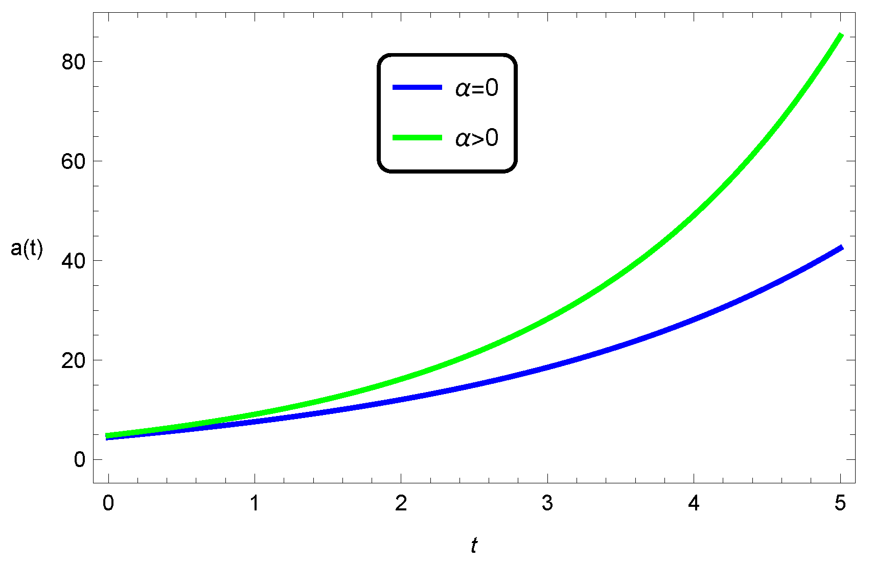
In Figure 5, we demonstrate the evolution of the scale factor in five-dimensional EGB gravity for the three spatial curvatures and a nonvanishing cosmological constant. It can be seen that for the open and closed universes, the increase is greater than for the flat universe, indicating that the presence of spatial curvature has an effect on this increase. In Figure 6, the energy density is depicted with the cosmological constant and, similarly to the general relativity case, only the open universe has physically acceptable behaviour; the closed universe violates the null energy condition, in that the energy density is negative. For the flat universe, the energy density vanishes identically. 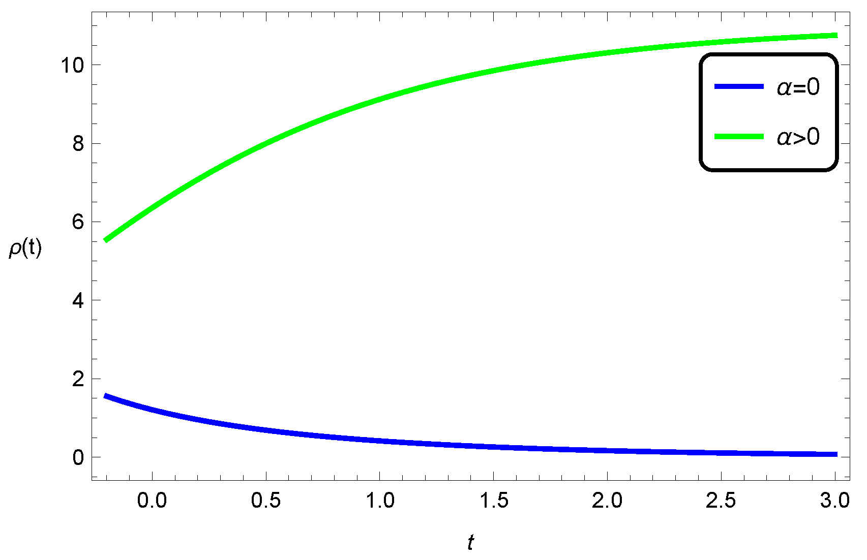Figure 7 depicts the comparative behaviour of the energy densities of the closed universe between EGB gravity and general relativity, with the cosmological constant. Both are positive and well-behaved functions, with the general relativistic case being decreasing, and the EGB scenario being a gradually increasing function; the Gauss–Bonnet corrections are directly contributing to an increasing energy density over cosmic time. 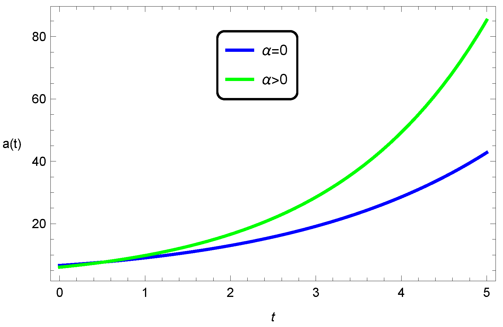Figure 8, Figure 9 and Figure 10 depict the scale-factor evolution in general relativity against the EGB universe. In all cases, the EGB contributions enhance the rate of the expansion.

5. Discussion

In this treatise, we analysed cosmological dust in higher-dimensional general relativity and EGB gravity. We showed that the model dynamics were governed by an Abel differential equation of the second kind, which was solved in general for all spacetime dimensions and spatial curvature to generate solutions for the scale factor. A general first integral was found in the EGB theory, and explicit and implicit solutions for the scale factor are possible, depending on the presence of the cosmological constant. Graphical plots were generated for the scale factor and the energy density in both general relativity and EGB gravity for several dimensions to probe the behaviour and evolution of these quantities over cosmic time. Due to the exponential nature of the solutions with nonvanishing $\mathrm{\Lambda }$, the scale factor was shown to increase over time, for all spatial curvature, indicating an expanding universe; the Gauss–Bonnet corrections contributed to the rate of expansion. We also note that for the open universe, the energy density in both general relativity and EGB gravity was negative for $\mathrm{\Lambda }\ne 0$, which is unphysical. A negative pressure is acceptable for a dark energy-type equation of state, which is something we aim to analyse in a subsequent treatise.