Abstract
We report the latest results on particle mixing in quantum field theory on curved spacetimes. We highlight possible connections with dark matter and dark energy. Furthermore, we present two indirect methods to observe these phenomena: one using non-relativistic neutrinos and the other employing an atomic analogue.
1. Introduction
The problems of dark matter and dark energy represent some of the most profound and puzzling challenges in modern cosmology and astrophysics. Both concepts arose out of the need to explain several large-scale observations that cannot be satisfactorily accounted for by current physical theories. The -cold dark matter (CDM) model, widely supported by observational evidence, suggests that dark energy constitutes approximately 68% of the total energy density of the universe [1]. In this model, the cosmological constant acts as dark energy, fueling the accelerated expansion of the universe [2,3,4,5,6,7]. Instead, dark matter was introduced to reconcile the discrepancies between the mass estimates of clusters and galaxies derived from kinematic measurements and those inferred from luminosity data. The existence of dark matter, as originally proposed by Trimble [8], is inferred primarily from its gravitational effects, as it has not been directly observed. Dark matter constitutes about 26% of the energy density of the universe, starkly contrasting with the 5% contributed by baryonic matter [9,10,11,12,13,14,15,16,17,18,19,20,21,22,23,24,25,26,27].
The nature of dark matter, in particular, has given rise to a wide number of theoretical proposals, each with different origins and implications. Among these models, some postulate the existence of entirely new particles beyond the Standard Model [28,29,30,31]. Supersymmetric extensions of the Standard Model [32,33,34,35,36,37,38,39,40,41,42,43,44,45,46,47], for instance, predict a rich spectrum of particles, with the lightest supersymmetric particle often identified as a stable and weakly interacting dark matter candidate. Other examples include axions and axion-like particles [48,49,50,51,52,53,54,55,56,57,58,59,60,61,62,63], which were originally introduced as a solution to the strong CP problem in quantum chromodynamics, but have since proved to be compelling candidates for dark matter. Others are based on condensation mechanisms that emerge in quantum field theory (QFT), invoking the non-trivial structure of the vacuum, including effects arising from flavour fermion mixing [64,65,66,67,68,69,70,71]. In recent years, a novel connection between flavour fermion mixing and cosmology has gained significant attention. One of the potential QFT models for flavour fermion mixing, formulated within the framework of the flavour Hilbert space [72,73,74,75,76,77], involves a condensed vacuum state known as the flavour vacuum. This vacuum state, due to its condensate structure, introduces a new contribution to the energy-momentum tensor, and it can be shown that for a wide range of spacetime metrics it attains the form of a classical perfect fluid with vanishing pressure. In a similar way, it has been shown that the flavour vacuum of mixed bosons could, in principle, represent a component of the dark energy [70]. Testing the contribution of mixed fermions, such as neutrinos, to dark matter poses significant challenges. This difficulty arises because the condensate energy only becomes relevant at cosmological scales, and because the fermions involved (e.g., neutrinos) are notoriously difficult to control experimentally.
In this review, we revisit two different approaches to evaluating the contribution of the flavour vacuum to dark matter. The first approach is based on the observation that the same mechanism that leads to flavour vacuum condensation also modifies neutrino oscillation formulas within QFT. However, while these corrections are generally negligible, they become relevant for non-relativistic neutrinos, since in natural units, the neutrino energy is of the same order as its mass , i.e., .
This limitation effectively rules out traditional oscillation experiments as a means of probing the condensation mechanism. However, experiments designed to detect non-relativistic neutrinos, such as PTOLEMY [78,79], could provide a platform where QFT effects become observable.
The second approach explores the possibility of identifying an analogous physical system that can be controlled under laboratory conditions. One promising candidate is a system consisting of an ensemble of independent Rydberg atoms interacting with laser light, which could mimic certain aspects of the flavour vacuum.
The paper is structured as follows: Section 2 introduces the QFT model for particle mixing based on the flavour Hilbert space and its connection to the dark components of the universe. This section establishes the notation and includes an analysis of the associated energy-momentum tensor. Section 3 examines the potential for low-energy neutrino experiments, such as PTOLEMY, to test the QFT of neutrino mixing and its associated dark matter-like contributions. Section 4 discusses the use of an analogous physical system, specifically, an ensemble of Rydberg atoms, atoms in which a valence electron occupies a state with a high principal quantum number , interacting with laser light, to investigate these effects. In Section 5, we draw our conclusions.
2. Mixing in QFT and Dark Components of the Universe
The main features of the QFT formalism for the fermion mixing are summarised below. For the sake of simplicity, we restrict ourselves to the two-flavour case and, without loss of generality, we choose the reference frame such that . In QFT, the usual mixing relations (in which and are promoted to fields) read:
where is the mixing angle are the fields with definite masses, respectively, and , and are the (electronic and muonic) flavour fields. The Equation (1) can be rewritten as , where and is the generator of mixing transformations. The flavour annihilation operators are defined as and . From the flavour operators, it is possible to define the so-called flavour vacuum as:
This is related to the ordinary mass vacuum (defined as the state annihilated by the operators with definite masses ) through the mixing generator as . The crucial point of this section is that the flavour vacuum, which is the physical one, presents a condensate structure of () fermions (antifermions) . and are the Bogoliubov coefficients of mixing, given by the scalar products of modes, respectively, and , with positive u and negative energy v. Explicitly:
where . One interesting consequence of the condensate structure of the flavour vacuum is that the flavour vacuum itself turns out to be unitary inequivalent to the mass vacuum . We now briefly recap the properties of the energy-momentum tensor associated to the flavour vacuum, first in flat and then in curved spacetime. The energy-momentum content of the flavour vacuum is characterised via the vacuum expectation value (VEV) , where normal ordering is with respect to the mass vacuum , which isolates the pure mixing contribution (see [66,68]). It should be noted that in general the energy-momentum tensor depends on two, generally distinct, time arguments t and , one associated with the fields and one characterising the flavour vacuum, . The energy-momentum tensor (operator) in a curved spacetime is:
For free fields, . On the other hand, for a wide range of metrics, including Minkowski, the VEV on the flavour vacuum is non-zero only for the 00 component, the energy density , and for all . In particular, the pressure of the flavour vacuum is equal to zero, . Thus, the equation of state gives an adiabatic index , as is the case for cold dark matter and more generally for non-relativistic matter, known in cosmology as dust. In flat spacetime, one has the explicit expression:
In recent analyses, the flavour vacuum has been studied in the Friedmann–Lemaître–Robertson–Walker (FLRW) metric [68].
Starting from the line element , where is the conformal time defined as with range corresponding to , can be written as (for the details, we refer to [68]):
where is the helicity and the momentum, and are solutions of the Dirac equation in the FRLW metric, and are the annihilation operators for particles and antiparticles and is an auxiliary tensor given by
Again, the tensor is non-zero only for . Therefore, this quantity can be interpreted as the energy-momentum tensor of a perfect fluid. Under the assumption of isotropy, this tensor has only two independent components: and . Considering the specific case where the cosmological scale factor follows an exponential evolution, with being the constant Hubble factor, we analyse the limit of . Approximating the result to first order in the conformal time , we obtain the following expression for the energy density :
where and are the Bogoliubov coefficients while the components are zero . Therefore, at the lowest order in , the adiabatic coefficient and, consequently, the energy-momentum tensor associated with the flavour vacuum satisfies the equation of state of a pressureless perfect fluid. In particular, as it is diagonal and conserved (satisfying the Bianchi identities), it can be interpreted as the relativistic tensor of a perfect fluid. In the specific case of the De Sitter background, it is demonstrated that this tensor adheres to the equation of state of dust and cold dark matter, indicating that it may constitute a component of cosmological dark matter.
This analysis has been extended recently to include astrophysical metrics [69], such as spherically symmetric spacetimes with and , arbitrary but sufficiently regular functions of R. Also, in this context, the only non-vanishing component of the VEV is :
where L is the flavour index, j is the total angular momentum, its projection, is the Dirac quantum number defined as for and for , and and are the solutions of the radial Dirac equation, and for the q contribution, we have . Interestingly, if the weak field approximation is taken into account, one can obtain a modification of the gravitational potential, induced by the flavour vacuum, in the form of a Yukawa potential:
with a freely specifiable dimensionless parameter, , with G the Newtonian constant of gravitation, and K is the expectation value on the flavour vacuum of the component in the Minkowski metric, Equation (6). This extra term in the gravitational potential could account for both flat rotation curves and the baryonic Tully–Fisher relation [80,81,82].
In the framework of QFT, boson mixing also shows intriguing connections to the dark sector. Following a procedure similar to the one for the fermion mixing, one can compute the VEV of the energy momentum tensor within the FLRW metric.
In Ref. [70], the complete computation has been performed, showing that the energy-momentum tensor is diagonal and, therefore, it behaves like a classical perfect fluid, whose properties depend on the metric. Moreover, can be considered as a source term for the Einstein field equations, since it satisfies the Bianchi identity. Considering a de Sitter background, the values of the adiabatic factor of the boson flavour mixing are included in the interval . If one takes the flat spacetime limit, where and , and by definition flat space corresponds to , implying , when , the component of the energy-momentum tensor assumes the simple form:
leading to , which corresponds to a typical dark energy equation of state .
These results suggest a possible connection between purely quantum field theoretical effects and the dark components of the universe. Obtaining an experimental validation of these phenomena is, in principle, a challenging task, since they would be relevant only on cosmological scales. Nevertheless, in recent years, alternative routes towards an experimental verification of the above models have been proposed, and we now proceed to review them.
Testing the possible contribution of the mixed fermion condensate to dark matter directly is a challenge of considerable difficulty. The major difficulties are related to the fact that the fermions involved, namely, neutrinos, are elusive, and also to the fact that the condensate energy is relevant only on cosmological scales. We review two different approaches to this problem; the first relies on an analysis of the condensate effects in low-energy neutrinos through the process of neutrino capture on tritium; the second is centered on the determination of an atomic analogue to flavour fermion mixing.
3. Neutrino Capture on Tritium
The first method to probe the QFT of neutrino mixing and its potential connection to dark matter involves conducting low-energy neutrino experiments, such as those proposed by the PTOLEMY project [78]. Specifically, our focus is on examining the QFT condensation effect on the detection process, represented by neutrino capture on tritium. We consider non-relativistic (low energy) neutrinos, which constitute the cosmic neutrino background and may be probed by the PTOLEMY experiment. The fundamental process for neutrino capture is the inverse beta decay, where a neutrino interacts with a neutron to produce an electron and a proton (). Because of the relatively low energies of the neutrinos, we can accurately describe this reaction using the current–current interaction Hamiltonian [79]:
where , , , are, respectively, the neutron, the proton, the electron and the neutrino field, is the Fermi constant, is the CKM matrix element, and and are nuclear form factors [83]. The tree level amplitude is usually defined as
where S denotes the scattering matrix, with subscripts labelling the matrix element between the initial state I and final state F, is the Kronecker delta, and the Dirac delta function enforces conservation of total four-momentum. Restricting to two neutrino flavours for simplicity, the electron-neutrino field can be expressed as with the mixing angle. The initial and final states for the inverse beta decay are
where the are momentum indices, the spin indices for . The different ways researchers approach neutrino mixing mainly stem from how they define the flavour states of neutrinos. We can categorise these variations into four cases: Firstly, there are Decoupled Pontecorvo States, where neutrinos are initially produced as Pontecorvo flavour states. Due to the different propagation velocities and for the two mass components and , the initial coherent combination decoheres as it propagates. By the observation time, complete decoherence into mass eigenstates is observed. The resulting inverse beta decay takes the form . In this case, mixing effects are present only at the state level. Next, Pontecorvo States involve neutrinos being both produced and interacting as Pontecorvo flavour states. Mixing at the field level is considered “eternal” without decoherence. Neutrino states in the amplitude are expressed as . However, this definition overlooks the spinorial nature of the neutrino states and can be interpreted as the action of the flavour creation operator on the neutrino vacuum state. This is clearly in contrast with the QFT of flavour fields.
Within the Pontecorvo–Dirac formalism, mixing is introduced at the field-theoretic level, taking into account the spinor nature of neutrino states. The creation operator for an electron neutrino is defined by where denotes the Dirac inner product, and is the annihilation operator of the antineutrino . The coefficients and are scalar products and encode spinor overlaps. When applied to the vacuum, the operator creates the state This construction assumes a single neutrino vacuum, , annihilated by the operators , , , and . In the Flavour Fock Space formalism, mixing is introduced at the field level without decoherence. The electron-flavour creation operator retains the structure but the flavour state is defined by its action on a flavour vacuum , which is distinct from the mass vacuum . Since depends explicitly on time, all fields and states must include the appropriate time arguments. Only in this full construction does the vacuum itself yield a dark-matter contribution.
As the most comprehensive scheme—recovering the other approaches as special cases—we separate the mixing in the field expansion, from that in the state definition, noting that when both appear together. Since all other mixing prescriptions arise as limiting cases of this flavour Fock space model, we compute the S-matrix elements and associated cross-section within this unified framework. Let us address our attention to the unnormalised amplitude
The integration boundary T must be pushed to . Using the generic states of Equation (16), we can write:
We can readily compute the matrix elements corresponding to the neutron, proton, and electron states. However, for neutrino states, the situation is slightly different: the time-dependent nature of the flavour vacuum introduces two distinct time parameters, and , which refer to the initial and final times of the asymptotic states. Given the extremely brief timescales involved in weak interactions, it is a valid approximation to assume . Consequently, we set . By using the flavour neutrino field and the flavour annihilators, the neutrino matrix element is given by
where and and are the flat Bogoliubov coefficients. We use the notation and to differentiate between the mixing angles in the fields and in the states. Inserting the neutrino matrix element in Equation (18) and taking the infinite time limit , we find
where , , where are
Considering the neutron rest frame and neglecting the proton recoil, then the 4-momenta are . We also set , sum over the neutron and proton spins and average over the electron spin, in order to have the unpolarised cross- section. The differential cross-section is then:
where the functions A and B are defined in terms of the (positive) neutrino velocities , , , , . The integral over cancels all the B terms and, for the non-relativistic neutrinos considered here, , , and we can neglect the difference .
We then multiply Equation (21) by , and the Fermi function, , with , to obtain the capture cross-section
This equation represents the most general form for the capture cross-section.
We can now distinguish different cases based on the various approaches to neutrino mixing, previously exposed: In the first case of decoupled Pontecorvo states, as expected, the cross-section aligns with the outcome from the reference [79], demonstrating that Equation (22) constitutes a proper generalisation. Next, for the Pontecorvo states, the Bogoliubov coefficients behave in the following way , , and , and we observe that the difference from the previous case lies solely in the multiplicative factor. In the Pontecorvo–Dirac approach, the cross-section exhibits a nuanced dependence on the neutrino momentum through :
It is worth noting that the same outcome is derived in the flavour Fock space approach if the negative energy term is excluded. Finally, in the Flavour Fock space states, the cross-section is given by:
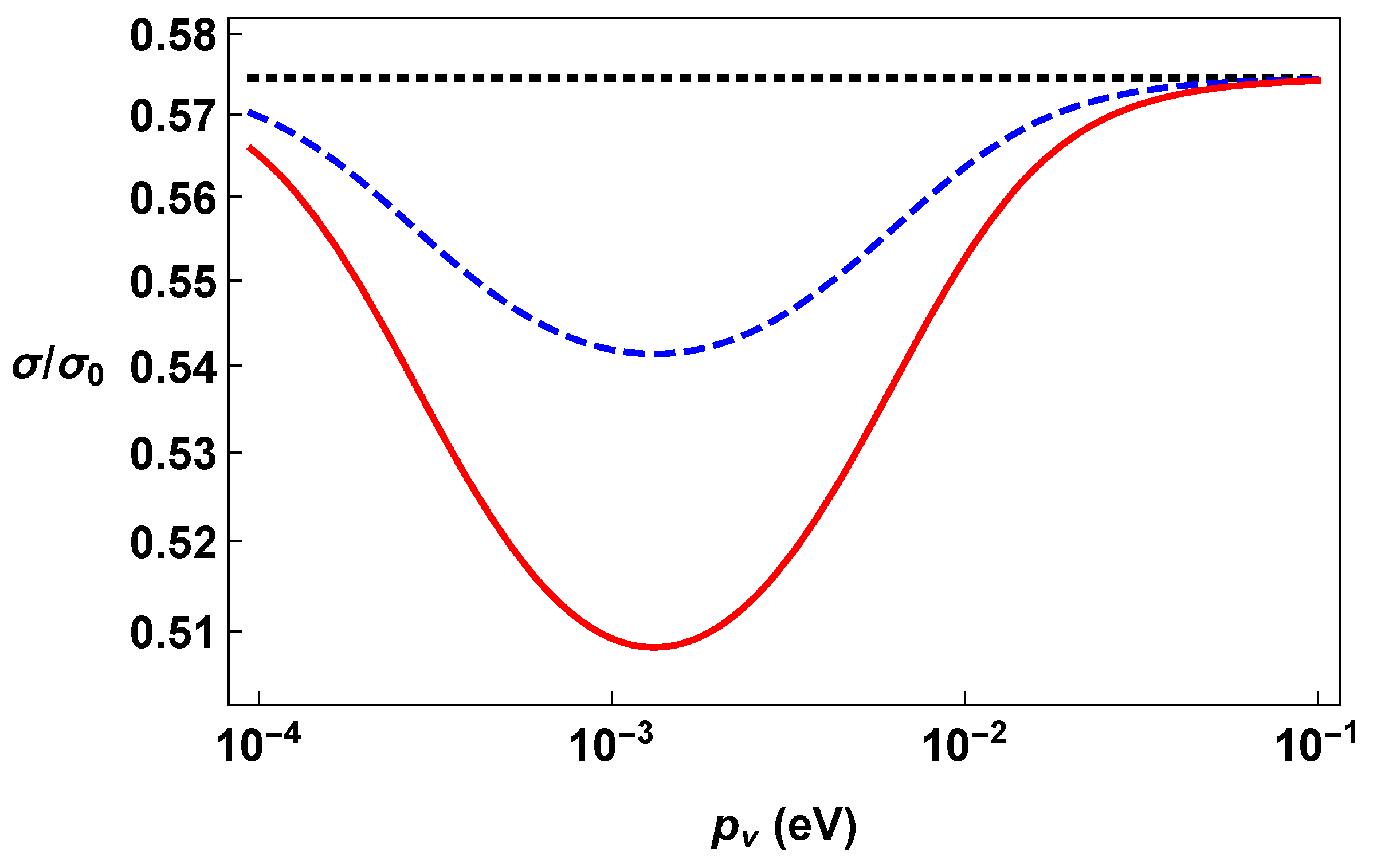
This result holds true under the assumption that the negative energy term represents a condensate hole term; otherwise, Equation (23) is obtained. Observe that the cross-section has a direct dependence on the square modulus of the Bogoliubov coefficient . Therefore, the same mechanism present at the base of the condensate generates a correction to the cross-section. The plot of the various cross-sections as a function of the neutrino momentum is shown in Figure 1. From the figure, it can be seen that the red graph (i.e., the cross-section in Fock space) has a minimum with respect to the Pontecorvo cross-section (dashed in black) and the blue dashed Pontecorvo–Dirac cross-section (without condensate), precisely because of the mechanism at the origin of the condensate. The expectation value of the number operator on the empty state is proportional to the square modulus of the Bogoliubov coefficient , as can be seen from the following relation: . Therefore, we retain that if the condensate effect is present, this could be a way to detect it.
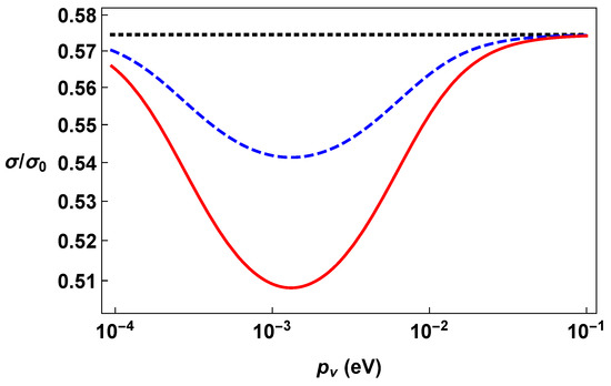
Figure 1.
The plot illustrates how the ratio of changes with neutrino momentum across the range of eV. The Pontecorvo cross-section is represented by the black dotted line, corresponding to . Meanwhile, the blue dashed line signifies the Pontecorvo–Dirac cross section, , and the red solid line depicts the Flavour Fock space cross-section labelled as . The ratio , representing the cross-section for decoupled neutrinos, remains constant at 1 and is not explicitly shown on the plot. Parameters include , eV2, and eV.
The capture rate on a sample of tritium of mass can be expressed in terms of the capture cross-section as
where represents the total count of tritium nuclei in the sample, and denotes the (differential) density of neutrinos per available energy state. It is important to note that the definition, provided in Equation (25), does not explicitly incorporate the velocity of neutrinos, which is inherent in the neutrino flux. This omission is due to the fact that the neutrino velocity is already implicitly factored into the capture cross-section . Under the sudden freeze-out approximation, the phase space distribution of neutrinos corresponds to the redshifted distribution function observed during the decoupling epoch. At a redshift z, the number density is given by:
where the integration over solid angle has been carried out in the final step.
Here, , and with the label denoting the quantities at the freeze-out.
We note that, strictly speaking, the distribution in Equation (26) should be written in terms of the neutrino energies rather than the momentum . However, since the freeze-out temperature is much larger than the neutrino masses , those masses are typically neglected.
At the current epoch , we have
where and eV. Finally, the differential capture rate becomes
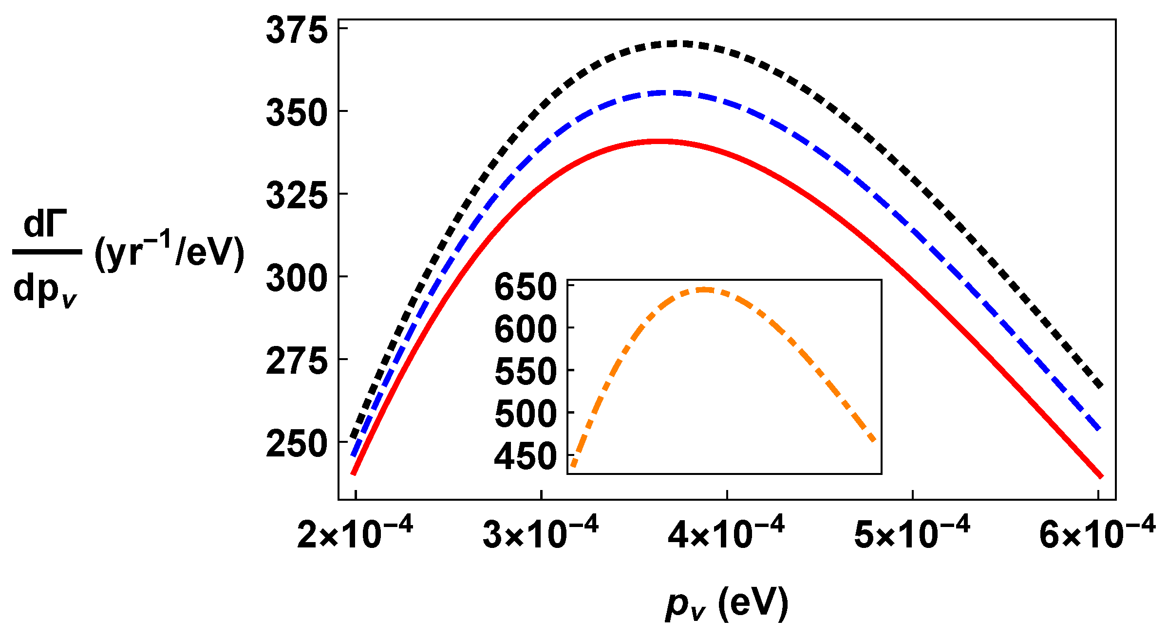
with the capture cross-section . Therefore, the same mechanism present at the base of the condensate generates a correction to the cross-section and, consequently, this correction must also be present in the capture rate. In Figure 2, we plot the differential capture rate for the various schemes discussed above. At higher momenta, all three curves depicted in Figure 2 converge toward the Pontecorvo result (the black dotted line).
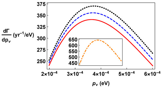
Figure 2.
The graph illustrates the differential capture rate , plotted against the neutrino momentum , ranging from to eV. Although dimensionless, the rate is expressed in units of yr−1 eV for easier comparison with prior findings. The Pontecorvo cross-section , is depicted by the black dotted line, while the Pontecorvo–Dirac cross-section , is represented by the blue dashed line. The red solid line corresponds to the Flavour Fock Space cross-section, . Furthermore, the inset features the capture rate (orange dot-dashed line) associated with the decoupled Pontecorvo cross-section. The analysis assumes a tritium sample with a total mass g. Other parameters remain consistent with those presented in Figure 1.
4. Rydberg Atoms
This section illustrates an alternative methodology for assessing the role of the condensate of mixed fermions, such as neutrinos, in the context of dark matter. This approach is founded upon the formal analogy that exists between independent Rydberg atoms interacting with a laser light and the mixing of fermions in the context of QFT. Rydberg atoms are atoms whose electrons are in an excited state, characterised by a very large principal quantum number, represented by the symbol n [84,85,86,87,88]. For , the energy of a Rydberg atom is given by , where is the Rydberg constant and is a corrective factor, called the quantum defect, which is negligible except for (see references [85,86,87]). In the case of a total spin of , the atom is fermionic. This is the case for alkaline atoms. In the following, we will consider a set of independent Rydberg atoms at a very low density and low temperature in order to avoid the interaction between them and also all the finite temperature effects. This approach allows us to neglect the interaction among the atoms and the finite temperature effects. The atoms interact with a laser light with Rabi frequency, , and detuning, . The laser light couples two levels of the atoms, for instance, the ground state and the first excited state (which we will refer to as and ), with . In QFT, these states are promoted to fields, with the total Hamiltonian being expressed as a sum of one-particle operators describing a single atom. Furthermore, the single-atom Hamiltonian can be separated into two distinct contributions: one for the centre-of-mass Hamiltonian, denoted as , and the other for the outer electron, represented by . We assume that the centre-of-mass Hamiltonian is that of free Dirac fields:
where m stands for the mass of the atom considered. The electronic part of the Hamiltonian is [88]
where is a doublet of free fermion fields and M is a matrix given by:
with . In this context, the M matrix plays the role of the mixing matrix. The Hamiltonian (30) can be diagonalised by means of a rotation:
where the “mixing angle” is . The fields, with , play the role of flavour neutrino fields and the fields, with , play the role of mass neutrino fields. The electron Hamiltonian explicitly becomes
where
By means of the rotation, the total Hamiltonian can be decomposed into the sum of two free Dirac Hamiltonian with masses and . Thus, atomic fields can be expanded into plane waves of mass
where are the solutions of Dirac equation for the free fields. The creation and annihilation operators undergo a trivial time evolution, i.e., . With these fields expansion, the total Hamiltonian is given by:
To conclude the formal analogy between the QFT description of Rydberg atoms and the QFT description of neutrino mixing, we can recast the rotation by means of the mixing generator and write . The mixing generator is given by:
This operator preserves the usual anticommutation relation and, at finite volume, is unitary. Moreover the action of this generation is equivalent to a Bogoliubov transformation nested into a rotation: , . The generator connects the representations associated with the “flavour” fields , and the “mass” fields ,. In particular, the vacuum in the two representations is related by means of the transformation . As in the case of fermion mixing, the VEV for the mixed fields of the energy momentum tensor for free Rydberg atoms is diagonal, with the only non-zero component given by the 00 component, as shown in Equation (6):
where and K is the cut-off on the momenta. By integrating over the whole space occupied by the condensate, the energy contribution, denoted by U, is obtained. By deriving U with respect to temperature T, it is possible to assess the contribution of the condensate to the thermal capacity of the system. Neglecting the finite effects of temperature, U turns out to be independent of the latter. However, a first approximation of the thermal effects can be obtained by introducing a temperature-dependent cut-off. This can be justified because as the temperature increases, the average energy increases, and consequently states with higher momenta are populated. Therefore, it is reasonable to assume that the cut-off must increase as T increases. In the simplest case of linear dependence of the cut-off K on temperature, given by , the contribution to the specific heat at constant volume due to the vacuum energy of mixed atoms is as follows:
where V is the volume of the gas of Rydberg atoms. Several peculiarities emerge regarding this contribution to the thermal capacity of the system, which deviate from conventional expectations. In particular, most notable is its dependence not on the number of constituent atoms, but on the volume of the condensate. This peculiar characteristic derives from its connection with the condensate’s vacuum energy, which corresponds to the continuous creation and annihilation of virtual Rydberg atom pairs from the vacuum. The abundance of such pairs scales with the volume occupied by the condensate and remains independent of the actual number of Rydberg atoms present. Consequently, given the zero pressure of the condensate, it follows from the first law of thermodynamics that , thus also linking entropy to volume. This quantum aspect of the entropy field [89] can manifest counterintuitive behaviour, requiring careful consideration when interpreting the heat capacity expression given in Equation (39) added to the ordinary terms, among which the one of a Fermi gas with two Rabi coupled components.
The QFT of particle mixing also predicts corrections to the oscillation formulae. In particular, the charge operators for ground and excited Rydberg fields are as follows:
Following the prescriptions of the section above, the oscillation formulae are and , where . In this equation, a high frequency oscillation term proportional to is visible. This QFT correction to the oscillation formulae could, in principle, be tested experimentally.
5. Conclusions
In this article, we have reviewed some key results for particle mixing in QFT, with a focus on its potential links to dark matter and dark energy. Given the inherent challenges in testing the contribution of mixed fermions to dark matter, we have explored two different approaches to probe these effects in the laboratory. The first approach focuses on low-energy neutrino capture experiments. We have considered different neutrino mixing schemes and the corresponding flavour state definitions in the calculation of neutrino absorption rates by tritium. Experiments such as PTOLEMY therefore have the potential to provide indirect evidence for flavour condensates and dark matter contributions induced by neutrino mixing. In the second approach reviewed, we have investigated the possibility of identifying a controllable physical system analogous to fermion mixing. Furthermore, its flavour vacuum has a non-trivial energy, leading to an additional contribution to the thermal capacity of the Rydberg atom ensemble that is directly related to this vacuum energy. These two complementary approaches offer promising avenues for exploring the interplay between fermion mixing, flavour condensates, and their potential implications for dark matter.
Author Contributions
Conceptualization, Writing, Review, and Editing: A.C., S.M., G.P., A.Q. and R.S.; Supervision, A.C. All authors have read and agreed to the published version of the manuscript.
Funding
This research received no external funding.
Data Availability Statement
This paper is a theoretical paper without generated data.
Acknowledgments
A.C., A.Q. and R.S. acknowledge partial financial support from MIUR and INFN. A.C. also acknowledge the COST Action CA1511 Cosmology and Astrophysics Network for Theoretical Advances and Training Actions (CANTATA).
Conflicts of Interest
The authors declare no conflicts of interest.
References
- Ade, P.A.R. et al. [Planck Collaboration] Planck 2015 results. XIII. Cosmological parameters. Astron. Astrophys 2016, 594, A13. [Google Scholar] [CrossRef]
- De Bernardis, P.; Ade, P.A.; Bock, J.J.; Bond, J.R.; Borrill, J.; Boscaleri, A.; Cobleet, K.; Crill, B.P.; De Gasperis, G.; Farese, P.C.; et al. A flat Universe from high-resolution maps of the cosmic microwave background radiation. Nature 2000, 404, 955. [Google Scholar] [CrossRef] [PubMed]
- Spergel, D.N.; Verde, L.; Peiris, H.V.; Komatsu, E.; Nolta, M.R.; Bennett, C.L.; Halpern, M.; Hinshaw, G.; Jarosik, N.; Kogut, A.; et al. First-Year Wilkinson Microwave Anisotropy Probe (WMAP) Observations: Determination of Cosmological Parameters. Astrophys. J. Suppl. Ser. 2003, 148, 175. [Google Scholar] [CrossRef]
- Dodelson, S.; Narayanan, V.K.; Tegmark, M.; Scranton, R.; Budavari, T.; Connolly, A.; Csabai, I.; Eisenstein, D.; Frieman, J.A.; Gunn, J.E.; et al. The Three-dimensional Power Spectrum from Angular Clustering of Galaxies in Early Sloan Digital Sky Survey Data. Astrophys. J. 2002, 572, 140. [Google Scholar] [CrossRef]
- Szalay, A.S.; Jain, B.; Matsubara, T.; Scranton, R.; Vogeley, M.S.; Connolly, A.; Dodelson, S.; Eisenstein, D.; Frieman, J.A.; Gunn, J.E.; et al. Karhunen-Loève Estimation of the Power Spectrum Parameters from the Angular Distribution of Galaxies in Early Sloan Digital Sky Survey Data. Astrophys. J. 2003, 591, 1. [Google Scholar] [CrossRef]
- Peebles, P.J.E.; Ratra, B. The cosmological constant and dark energy. Rev. Mod. Phys. 2003, 75, 559. [Google Scholar] [CrossRef]
- Riess, A.G.; Strolger, L.; Tonry, J.; Casertano, S.; Ferguson, H.C.; Mobasher, B.; Challis, P.; Filippenko, A.V.; Jha, S.; Li, W.; et al. Type Ia Supernova Discoveries at z>1 from the Hubble Space Telescope: Evidence for Past Deceleration and Constraints on Dark Energy Evolution. Astrophys. J. 2004, 607, 665. [Google Scholar] [CrossRef]
- Trimble, V. Exotic dark matter in the universe. Annu. Rev. Astron. Astrophys. 1987, 25, 425–472. [Google Scholar] [CrossRef]
- Hinshaw, G.; Larson, D.; Komatsu, E.; Spergel, D.N.; Bennett, C.L.; Dunkley, J.; Nolta, M.R.; Halpern, M.; Hill, R.S.; Odegard, N.; et al. Nine-Year Wilkinson Microwave Anisotropy Probe (WMAP) Observations: Cosmological Parameter Results. Astrophys. J. Suppl. Ser. 2013, 208, 19. [Google Scholar] [CrossRef]
- Hin, T.; Gupta, V. The Dark Matter: A Review of Current Understanding. Phys. Rep. 2020, 843, 1–54. [Google Scholar]
- Bertone, G.; Hooper, D.; Silk, J. Particle dark matter: Evidence, candidates and constraints. Phys. Rep. 2005, 405, 279. [Google Scholar] [CrossRef]
- D’amico, G.; Kamionkowski, M.; Sigurdson, K. Dark matter astrophysics. arXiv 2012, arXiv:0907.1912(2012). [Google Scholar]
- Bertone, G. Particle Dark Matter: Observation, Models and Searches; Cambridge University Press: Cambridge, UK, 2010. [Google Scholar]
- Bottino, A.; Fornengo, N. Dark matter and its particle candidates. lectures published in Trieste 1998, non-accelerator particle physics. arXiv 1988, arXiv:hep-ph/9904469. [Google Scholar]
- Feng, J.L. Dark Matter Candidates from Particle Physics and Methods of Detection. Ann. Rev. Nuc. Part. Sci. 2010, 48, 495–545. [Google Scholar] [CrossRef]
- Chang, J.; Ambrosi, G.; An, Q.; Asfandiyarov, R.; Azzarello, P.; Bernardini, P.; Bertucci, B.; Cai, M.S.; Caragiulo, M.; Chen, D.Y.; et al. The DArk Matter Particle Explorer mission. Astrop. Phys. 2017, 95, 6–24. [Google Scholar] [CrossRef]
- Profumo, S.; Giani, L.; Piattella, O.F. An Introduction to Particle Dark Matter. Universe 2019, 5, 213. [Google Scholar] [CrossRef]
- Bertone, G.; Tait, T.M.P. A new era in the search for dark matter. Nature 2018, 562, 51–56. [Google Scholar] [CrossRef]
- Hooper, D. Particle Dark Matter; The Dawn of the LHC Era: Boulder, CO, USA, 2010; pp. 709–764. [Google Scholar]
- Boehm, C.; Fayet, P.; Silk, J. Light and heavy dark matter particles. Phys. Rev. D 2004, 69, 101302. [Google Scholar] [CrossRef]
- Arkani-Hamed, N.; Finkbeiner, D.P.; Slatyer, T.R.; Weiner, N. A theory of dark matter. Phys. Rev. D 2009, 79, 015014. [Google Scholar] [CrossRef]
- Khoury, J. Alternative to particle dark matter. Phys. Rev. D 2015, 91, 024022. [Google Scholar] [CrossRef]
- Comelli, D.; Pietroni, M.; Riotto, A. Dark energy and dark matter. Phys. Lett. B 2003, 571, 115–120. [Google Scholar] [CrossRef]
- Farrar, G.R.; Peebles, P.J.E. Interacting Dark Matter and Dark Energy. Astroph. J. 2004, 604, 1. [Google Scholar] [CrossRef]
- Baudis, L. Dark matter detection. J. Phys. G Nucl. Part Phys. 2016, 43, 044001. [Google Scholar] [CrossRef]
- Hui, L. Wave dark matter. Ann. Rev. Astr. Astroph. 2021, 59, 247–289. [Google Scholar] [CrossRef]
- Gaskins, J.M. A review of indirect searches for particle dark matter. Contemp. Phys. 2016, 57, 496–525. [Google Scholar] [CrossRef]
- Capolupo, A.; Pisacane, G.; Quaranta, A.; Romeo, F. Probing mirror neutrons and dark matter through cold neutron interferometry. Phys. Dark Universe 2024, 46, 101688. [Google Scholar] [CrossRef]
- Capolupo, A.; Quaranta, A.; Serao, R. The impact of the X17 boson on particle physics anomalies: Muon anomalous magnetic moment, Lamb shift and W mass. Phys. Dark Universe 2025, 47, 101748. [Google Scholar] [CrossRef]
- Iwamoto, S.; Seller, K.; Trócsányi, Z. Sterile neutrino dark matter in a U(1) extension of the standard model. J. Cosmol. Astropart. Phys. 2022, 1, 35. [Google Scholar] [CrossRef]
- Ilten, P.; Soreq, Y.; Williams, M.; Xue, W. Serendipity in dark photon searches. J. High Energy Phys. 2018, 6, 4. [Google Scholar] [CrossRef]
- Huang, P.; Wagner, C.E.M. Blind spots for neutralino dark matter in the MSSM with an intermediate mA. Phys. Rev. D 2014, 90, 015018. [Google Scholar] [CrossRef]
- Low, M.; Wang, L.T. Neutralino dark matter at 14 TeV and 100 TeV. J. High Energy Phys. 2014, 2014, 161. [Google Scholar] [CrossRef]
- Enqvist, K.; Mazumdar, A. Cosmological consequences of MSSM flat directions. Phys. Rep. 2003, 380, 99–234. [Google Scholar] [CrossRef]
- Roszkowski, L.; Sessolo, E.M.; Trojanowski, S. WIMP dark matter candidates and searches- current status and future prospects. Rep. Prog. Phys. 2018, 81, 066201. [Google Scholar] [CrossRef] [PubMed]
- Carroll, S.M. The cosmological constant. Liv. Rev. Relativ. 2001, 4, 1. [Google Scholar] [CrossRef]
- Dolan, M.J.; Kahlhoefer, F.; McCabe, C.; Schmidt-Hoberg, K. A taste of dark matter: Flavour constraints on pseudoscalar mediators. J. High Energ. Phys. 2015, 2015, 171. [Google Scholar] [CrossRef]
- Martin, S.P. A supersymmetry primer. Adv. Ser. Direct. J. High Energy Phys. 1998, 18, 1. [Google Scholar]
- Beekveld, M.V.; Caron, S.; Austri, R.R.D. The current status of fine-tuning in supersymmetry. J. High Energ. Phys. 2020, 2020, 147. [Google Scholar] [CrossRef]
- Baer, H.; Barger, V.; Huang, P.; Tata, X. Natural supersymmetry: LHC, dark matter and ILC searches. J. High Energ. Phys. 2012, 2012, 109. [Google Scholar] [CrossRef]
- Munoz, C. Model of supersymmetry for dark matter. EPJ Web Conf. 2017, 36, 01002. [Google Scholar] [CrossRef]
- Gomez, M.E.; Lazarides, G.; Pallis, C. yukawa quasi-unification. Nucl. Phys. B 2002, 638, 165–185. [Google Scholar] [CrossRef]
- Lopez, J.L.; Yuan, K.; Nanopoulos, D.V. SUSY guts dark matter. Nucl. Phys. B 1991, 267, 2. [Google Scholar] [CrossRef]
- Feng, J.L.; Matcvhev, K.T.; Wilczek, F. Neutralino dark matter in focus point supersymmetry. Phys. Lett. B 2000, 482, 4. [Google Scholar] [CrossRef]
- Nath, P.; Arnowitt, R. Nonuniversal soft supersymmetry breaking and dark matter. Phys. Rev. D 1997, 56, 5. [Google Scholar] [CrossRef]
- Cohen, T.; Lisanti, M.; Pierce, A.; Slatyer, T.R. Wino dark matter under siege. J. Cosmol. Astropart. Phys. 2013, 2013, 061. [Google Scholar] [CrossRef]
- Fan, J.; Reece, M. In wino veritas? Indirect searches shed light on neutralino dark matter. J. High Energ. Phys. 2013, 2013, 124. [Google Scholar] [CrossRef]
- Perivolaropoulos, L.; Skara, F. Challenges for ΛCDM: An update. New Astron. Rev. 2022, 95, 101659. [Google Scholar] [CrossRef]
- Misiaszek, M.; Rossi, N. Direct detection of dark matter: A critical review. Symmetry 2024, 16, 201. [Google Scholar] [CrossRef]
- Oikonomou, V.K. Effects of the axion through the Higgs portal on primordial gravitational waves during the electroweak breaking. Phys. Rev. D 2023, 107, 064071. [Google Scholar] [CrossRef]
- Pandey, S.; Hall, E.D.; Evans, M. First results from the axion dark-matter birefringent cavity (ADBC) experiment. Phys. Rev. Lett. 2024, 133, 111003. [Google Scholar] [CrossRef]
- Oswald, R.; Nevsky, A.; Vogt, V.; Schiller, S.; Figueroa, N.; Zhang, K.; Tretiak, O.; Antypas, D.; Budker, D.; Banerjee, A.; et al. Search for dark matter induced oscillations of fundamental constant using molecular spectroscopy. Phys. Rev. Lett. 2022, 129, 031302. [Google Scholar] [CrossRef]
- Dror, J.A.; Gori, S.; Munbodh, P. QCD axion-mediated dark matter. J. High Energy Phys. 2023, 2023, 128. [Google Scholar] [CrossRef]
- Peccei, R.D.; Quinn, H. CP conservation in the presence of pseudoparticles. Phys. Rev. Lett. 1977, 38, 1440. [Google Scholar] [CrossRef]
- Peccei, R.D.; Quinn, H. Constraints imposed by CP conservation in the presence of pseudoparticles. Phys. Rev. D 1977, 16, 1791. [Google Scholar] [CrossRef]
- Weinberg, S. A New Light Boson? Phys. Rev. Lett. 1978, 40, 223. [Google Scholar] [CrossRef]
- Wilczek, F. Problem of strong P and T invariance in the presence of instantons. Phys. Rev. Lett. 1978, 40, 279. [Google Scholar] [CrossRef]
- Raffelt, G.G. Axions- motivation, limits and searches. J. Phys. A 2007, 40, 6607. [Google Scholar] [CrossRef]
- Marsch, D.J.E. Axion Cosmology. Phys. Rep. 2016, 643, 1–79. [Google Scholar] [CrossRef]
- Kim, J.E. Weak-Interaction Singlet and Strong CP Invariance. Phys. Rev. Lett. 1979, 43, 103. [Google Scholar] [CrossRef]
- Shifman, M.; Vainshtein, A.; Zakharov, V. Can confinement ensure natural CP invariance of strong interactions? Nucl. Phys. B 1980, 166, 493. [Google Scholar] [CrossRef]
- Zhitnitsky, A.R. On Possible Suppression of the Axion Hadron Interactions. Sov. J. Nucl. Phys. 1980, 31, 260. [Google Scholar]
- Dine, M.; Fischler, W.; Srednicki, M. A Simple Solution to the Strong CP Problem with a Harmless Axion. Phys. Lett. B 1981, 104, 199. [Google Scholar] [CrossRef]
- Capolupo, A.; Giampaolo, S.M.; Lambiase, G.; Quaranta, A. Probing quantum field theory particle mixing and dark-matter-like effects with Rydberg atoms. Eur. Phys. J. C 2020, 80, 423. [Google Scholar] [CrossRef]
- Capolupo, A.; Quaranta, A. Neutrino capture on tritium as a probe of flavor vacuum condensate and dark matter. Phys. Lett. B 2023, 839, 137776. [Google Scholar] [CrossRef]
- Capolupo, A.; Quaranta, A.; Serao, R. Field mixing in curved spacetime and Dark Matter. Symmetry 2023, 15, 807. [Google Scholar] [CrossRef]
- Capolupo, A.; Maria, G.D.; Monda, S.; Quaranta, A.; Serao, R. Quantum field theory of neutrino mixing in spacetime with torsion. Universe 2024, 10, 170. [Google Scholar] [CrossRef]
- Capolupo, A.; Carloni, S.; Quaranta, A. Quantum flavor vacuum in the expanding universe: A possible candidate for cosmological dark matter? Phys. Rev. D 2022, 105, 105013. [Google Scholar] [CrossRef]
- Capolupo, A.; Capozziello, S.; Pisacane, G.; Quaranta, A. Missing matter in galaxies as a neutrino mixing effect. Phys. Dark Universe 2025, 48, 101894. [Google Scholar] [CrossRef]
- Capolupo, A.; Quaranta, A. Boson mixing and flavor vacuum in the expanding universe: A possible candidate for the dark energy. Phys. Lett. B 2023, 840, 137889. [Google Scholar] [CrossRef]
- Capolupo, A.; Quaranta, A. Fermion condensate induced by axial interactions and cosmological implications. J. Phys. G. 2024, 51, 105202. [Google Scholar] [CrossRef]
- Alfinito, E.; Blasone, M.; Iorio, A.; Vitiello, G. Squeezed neutrino oscillations in quantum field theory. Phys. Lett. B 1995, 362, 91–96. [Google Scholar] [CrossRef]
- Blasone, M.; Vitiello, G. Quantum field theory of fermion mixing. Ann. Phys. 1995, 244, 283–311. [Google Scholar] [CrossRef]
- Blasone, M.; Capolupo, A.; Vitiello, G. Quantum field theory of three flavor neutrino mixing and oscillations with CP violation. Phys. Rev. D 2002, 66, 025033. [Google Scholar] [CrossRef]
- Blasone, M.; Capolupo, A.; Capozziello, S.; Carloni, S.; Vitiello, G. Neutrino mixing contribution to the cosmological constant. Phys. Lett. A 2004, 323, 182–189. [Google Scholar] [CrossRef]
- Ji, C.-R.; Mishchenko, Y. The general theory of quantum field mixing. Phys. Rev. D 2002, 65, 096015. [Google Scholar] [CrossRef]
- Capolupo, A.; Ji, C.-R.; Mishchenko, Y.; Vitiello, G. Phenomenology of flavor oscillations with non-perturbative effects from quantum field theory. Phys. Lett. B 2004, 594, 135–140. [Google Scholar] [CrossRef]
- Betti, M.G. et al. [PTOLEMY Collaboration] Neutrino physics with the PTOLEMY project: Active neutrino properties and the light sterile case. arXiv 2019, arXiv:1902.05508. [Google Scholar]
- Long, A.J.; Lunardini, C.; Sabancilar, E. Detecting non-relativistic cosmic neutrinos by capture on tritium: Phenomenology and physics potential. arXiv 2014, arXiv:1405.7654. [Google Scholar] [CrossRef]
- Jusufi, K.; Leon, G.; Millano, A.D. Dark Universe Phenomenology from Yukawa Potential? Phys. Dark Univ. 2023, 42, 101318. [Google Scholar] [CrossRef]
- Cardone, V.F.; Capozziello, S. Systematic biases on galaxy haloes parameters from Yukawa-like gravitational potentials. Mon. Not. Roy. Astron. Soc. 2011, 414, 1301. [Google Scholar] [CrossRef]
- Stabile, A.; Capozziello, S. Galaxy rotation curves in f(R,ϕ) gravity. Phys. Rev. D 2013, 87, 064002. [Google Scholar] [CrossRef]
- Zyla, P.A. et al. [Particle Data Group] Review of particle physics. Prog. Theor. Exp. Phys. 2020, 2022, 083C01. [Google Scholar]
- Gallagher, T.F. Rydberg atoms. Rep. Prog. Phys. 1988, 51, 143. [Google Scholar] [CrossRef]
- Han, J.; Jamil, Y.; Norum, D.V.L.; Tanner, P.J.; Gallagher, T.F. RB nf quantum defects from millimeter-wave spectroscopy of cold 85Rb Rydberg atoms. Phys. Rev. A 2006, 74, 054502. [Google Scholar] [CrossRef]
- Li, W.; Mourachko, I.; Noel, M.W.; Gallagher, T.F. Millimeter-wave spectroscopy of cold Rb Rydberg atoms in a magneto-optical trap: Quantum defects of the ns, np, and nd series. Phys. Rev. A 2003, 67, 052502. [Google Scholar] [CrossRef]
- Weber, K.-H.; Sansonetti, C.J. Accurate energies of nS, nP, nD, nF, and nG levels of neutral cesium. Phys. Rev. A 1987, 35, 4650. [Google Scholar] [CrossRef]
- Cui, J.; van Bijnen, R.; Pohl, T.; Montangero, S.; Calarco, T. Optimal control of Rydberg lattice gases. Quantum Sci. Technol. 2017, 2, 035006. [Google Scholar] [CrossRef]
- Umezawa, H.; Matsumoto, H.; Tachiki, M. Thermo Field Dynamics and Condensed States; North-Holland: New York, NY, USA, 1982. [Google Scholar]
Disclaimer/Publisher’s Note: The statements, opinions and data contained in all publications are solely those of the individual author(s) and contributor(s) and not of MDPI and/or the editor(s). MDPI and/or the editor(s) disclaim responsibility for any injury to people or property resulting from any ideas, methods, instructions or products referred to in the content. |
© 2025 by the authors. Licensee MDPI, Basel, Switzerland. This article is an open access article distributed under the terms and conditions of the Creative Commons Attribution (CC BY) license (https://creativecommons.org/licenses/by/4.0/).