Shadow Analysis of an Approximate Rotating Black Hole Solution with Weakly Coupled Global Monopole Charge

Abstract

In this paper, we investigate the shadow properties of a rotating black hole with a weakly coupled global monopole charge using a modified Newman–Janis algorithm. This study explores how these charge and rotational effects shape the black hole’s shadow, causal structure, and ergoregions, with implications for distinguishing it from Kerr-like solutions. Analysis of null geodesics reveals observable features that may constrain the global monopole charge and weak coupling parameters within nonminimal gravity frameworks. Observational data from M87* and Sgr A* constrain the global monopole charge and coupling constant to $0\le \gamma \lesssim 0.036$ and $-0.2\lesssim \alpha \le 0$, respectively.

1. Introduction

Black holes are among the most fascinating astrophysical phenomena predicted by general relativity (GR) and have been central to theoretical and observational research for decades. Observations of M87* [1] and Sgr A* [2] by the Event Horizon Telescope (EHT) collaboration have intensified interest in black holes, allowing us to probe their properties beyond theoretical models. Despite GR’s successes at cosmic scales, it faces significant limitations when addressing quantum effects, topological defects, and certain early-universe phenomena. For instance, GR does not inherently include quantum-scale phenomena or high-energy structures, such as global monopoles, which are predicted by symmetry-breaking mechanisms in various field theories [3,4]. These monopoles, arising from phase transitions in the early universe, are characterized by a global monopole charge (GMC) that affects spacetime geometry. The presence of the GMC meaningfully alters black hole properties, influencing thermodynamic behavior, stability, and observable features such as photon orbits and shadow boundaries [4,5,6]. Studying black holes with a GMC thus offers a valuable connection between gravitational and particle physics, revealing possible limitations of GR and suggesting pathways for developing modified gravitational theories. In fact, topological defects like global monopoles are predicted by grand unified theories and arise from the Kibble mechanism, which links defect formation to the breaking of specific symmetry groups during cosmological phase transitions [7,8]. A global monopole, resulting from the symmetry breaking of $\mathrm{SO}\left(3\right)$ to $\mathrm{U}\left(1\right)$, generates a unique gravitational effect that can be modeled by a Schwarzschild-like metric with an additional GMC term. This charge is connected to the symmetry-breaking energy scale and modifies spacetime by introducing a deficit angle, which affects the paths of test particles and the bending of light. Furthermore, the monopole’s core mass can be negative or negligible, leading to a repulsive gravitational effect that produces distinct features in black hole metrics. Additionally, in modified gravity theories, the gravitational influence of global monopoles has been extensively studied, particularly in models that incorporate matter-curvature coupling [9,10,11,12,13,14,15,16]. A recent study [17] in nonminimally coupled gravity showed that interactions between matter and geometry impart intriguing properties to global monopoles. In particular, the nonminimal coupling yields a positive core mass for the monopole and affects its internal structure, including core size. This study also examined the possibility of a nonminimal global monopole acting as an extra “hair” for a Schwarzschild black hole. By analyzing geodesic motion and gravitational light bending in the weak coupling regime, the study aimed to identify potential observational signatures of the GMC. This approach enables constraints on the nonminimal coupling and GMC parameters, providing insights into the symmetry-breaking scale. Recent work in Ref. [18] further investigated light propagation in the vicinity of this black hole, proposing observational limits on spacetime parameters.

Building on this interest in the impact of GMC on black hole properties, this paper examines the shadow of the rotating counterpart of this black hole. Analyzing the shadow of rotating black holes is essential, as it reveals observational signatures that can help differentiate various gravitational theories and enhance our understanding of spacetime geometry, especially in the presence of exotic features like topological defects. To obtain the rotating solution, we take the static metric introduced above as the seed and apply a modified version of the Newman–Janis algorithm (NJA) [19] to generate the rotating counterpart. This modified Newman–Janis algorithm (MNJA), as presented in Refs. [20,21], is particularly effective when extended to theories beyond GR, offering improved accuracy and stability in these contexts.

The paper is organized as follows: Section 2 provides an overview of the static black hole solution with a weakly coupled GMC, covering its spacetime and causal structure. In Section 3, we apply the MNJA step by step to derive the rotating counterpart of the static black hole. Section 4 examines the causal structure of the resulting spacetime, including horizon formation under varying black hole parameters, as well as the ergoregions and their evolution in terms of the GMC and coupling constant. Section 5 introduces the Lagrangian formalism and the Hamilton–Jacobi equation to study light propagation in the black hole’s exterior geometry. Here, we derive equations of motion for null geodesics and identify conditions for spherical photon orbits, mapping photon regions outside the event horizon and demonstrating the effects of the GMC on these regions. This section also parametrizes the celestial plane for an observer at infinity, enabling shadow boundary plots for several cases and detailed analysis of their properties. To facilitate observational testing, Section 6 introduces shadow observables and derives their mathematical expressions. We use these to constrain the GMC and coupling constant based on EHT data for M87* and Sgr A*. In Section 7, we calculate the black hole’s evaporation rate, considering parameter constraints inferred from EHT data. Finally, we summarize our findings in Section 8. Throughout this paper, we adopt natural units with $G=c=1=M_{\mathrm{pl}}$ and use a sign convention of $(-,+,+,+)$, with primes denoting differentiation with respect to the radial coordinate.

2. Static Black Hole Solution with GMC in the Weak Coupling Regime

The generalized theory of gravity incorporating nonminimal matter–curvature coupling is described by the action [22]

$$\mathcal{S}=\int {\mathrm{d}}^{4}x\sqrt{-g}\left\{{\displaystyle \frac{1}{2}}{f}_1\left(R\right)+[1+\alpha f_2\left(R\right){\mathcal{L}}_m]\right\},$$

(1)

where ${\mathcal{L}}_m$ is the matter Lagrangian density, $f_1\left(R\right)$ and $f_2\left(R\right)$ are arbitrary functions of the Ricci scalar, and $\alpha$ represents the interaction strength between $f_2\left(R\right)$ and ${\mathcal{L}}_m$, effectively measuring the nonminimal coupling strength. In Ref. [17], the specific choices $f_1\left(R\right)=R/\left(8\pi \right)$ and $f_2\left(R\right)=R$ were considered. For these values, an upper limit of $\left|\alpha \right|<5\times {10}^{-12}{\mathrm{m}}^2$ was derived in Ref. [23] based on nuclear physics considerations at high densities [24]. However, this limit is not applied in our study, as it pertains to environments with extreme densities not relevant here. Notably, setting $\alpha =0$ directly recovers GR for the above choices.

In Ref. [17], the matter Lagrangian density in Equation (1) was set as

$${\mathcal{L}}_m=-{\displaystyle \frac{1}{2}}{\partial }_{\mu }{\phi }^a{\partial }^{\mu }{\phi }^a-{\displaystyle \frac{1}{4}}\lambda {\left({\phi }^a{\phi }^a-{\eta }^2\right)}^2,$$

(2)

which corresponds to symmetry breaking from $\mathrm{SO}\left(3\right)$ to $\mathrm{U}\left(1\right)$, giving rise to a global monopole. Here, $\lambda$ and $\eta$ denote the Higgs field’s self-interaction constant and the symmetry-breaking energy scale, respectively. The Higgs field is represented by an isotriplet of scalar fields, ${\phi }^a=\eta h\left(r\right){\widehat{x}}^a$, where $a=1,2,3$ and $x^a=\left\{\sin \theta \cos \varphi ,\sin \theta \sin \varphi ,\cos \theta \right\}$ in Schwarzschild coordinates $(t,r,\theta ,\varphi )$. The radial function $h\left(r\right)$ satisfies $h\left(0\right)=0$ and $h(\infty )=1$. This symmetry allows us to consider the spherically symmetric line element

$$\mathrm{d}{s}^2=-B\left(r\right)\mathrm{d}{t}^2+{\displaystyle \frac{\mathrm{d}{r}^2}{A\left(r\right)}}+r^2\left(\mathrm{d}{\theta }^2+{\sin }^2\theta \mathrm{d}{\varphi }^2\right),$$

(3)

for analyzing the field equations. The metric functions $B\left(r\right)$ and $A\left(r\right)$ were derived in Ref. [17] by solving the field equations with this metric ansatz. Here, we specifically consider a weak matter–gravity coupling, where $\alpha f_2\left(R\right)=\alpha R<1$. Thus, we focus on small values of $\alpha$, satisfying the condition $\alpha <l_0^2$, where $l_0$ is a characteristic length scale, approximately the black hole mass, M. In this weak coupling framework, the global monopole is treated as a GMC for a black hole of mass M, and Ref. [17] provides solutions for $A\left(r\right)$ and $B\left(r\right)$ as

$$\begin{array}{ccc}& & A\left(r\right)\approx 1-\gamma -{\displaystyle \frac{2M}{r}}+{\displaystyle \frac{14\alpha \gamma }{r^2}}-{\displaystyle \frac{18\alpha \gamma M}{r^3}},\hfill \end{array}$$

(4)

$$\begin{array}{ccc}& & B\left(r\right)\approx 1-\gamma -{\displaystyle \frac{2M}{r}}+{\displaystyle \frac{20\alpha \gamma }{r^2}}-{\displaystyle \frac{30\alpha \gamma M}{r^3}},\hfill \end{array}$$

(5)

where $\gamma =8\pi {\eta }^2$ represents the deficit solid angle. As a result, the spacetime resembles a conical cosmic string with a one-dimensional topological defect. Consequently, this spacetime is asymptotically finite with a conical singularity, yet does not reduce to Minkowski spacetime at infinity. The parameter $\alpha$ has dimensions of length squared, while $\gamma$ is dimensionless. In the absence of the GMC (i.e., $\gamma =0$), the Schwarzschild black hole (SBH) solution is recovered. It is also important that ${\eta }^2<1$, ensuring that the symmetry-breaking scale remains below the Planck scale.

The black hole’s horizons occur where $g^{rr}=0$, yielding three solutions:

$$\begin{array}{ccc}& & {\mathrm{r}}_1={\displaystyle \frac{4}{1-\gamma }}\sqrt{{\displaystyle \frac{{\zeta }_2}{3}}}\cos \left({\displaystyle \frac{1}{3}}\arccos \left({\displaystyle \frac{2{\zeta }_3}{{\zeta }_2}}\sqrt{{\displaystyle \frac{3}{{\zeta }_2}}}\right)-{\displaystyle \frac{2\pi }{3}}\right)+{\displaystyle \frac{2M}{3(1-\gamma )}},\hfill \end{array}$$

(6)

$$\begin{array}{ccc}& & {\mathrm{r}}_2={\displaystyle \frac{4}{1-\gamma }}\sqrt{{\displaystyle \frac{{\zeta }_2}{3}}}\cos \left({\displaystyle \frac{1}{3}}\arccos \left({\displaystyle \frac{2{\zeta }_3}{{\zeta }_2}}\sqrt{{\displaystyle \frac{3}{{\zeta }_2}}}\right)\right)+{\displaystyle \frac{2M}{3(1-\gamma )}},\hfill \end{array}$$

(7)

$$\begin{array}{ccc}& & {\mathrm{r}}_3={\displaystyle \frac{4}{1-\gamma }}\sqrt{{\displaystyle \frac{{\zeta }_2}{3}}}\cos \left({\displaystyle \frac{1}{3}}\arccos \left({\displaystyle \frac{2{\zeta }_3}{{\zeta }_2}}\sqrt{{\displaystyle \frac{3}{{\zeta }_2}}}\right)-{\displaystyle \frac{2\pi }{3}}\right)+{\displaystyle \frac{4M}{3(1-\gamma )}},\hfill \end{array}$$

(8)

where

$$\begin{array}{ccc}\hfill & & {\zeta }_2={\displaystyle \frac{M^2}{3}}-{\displaystyle \frac{7\alpha }{2}}\left(1-\gamma \right)\gamma ,\hfill \end{array}$$

(9)

$$\begin{array}{ccc}& & {\zeta }_3={\displaystyle \frac{M^2}{27}}+{\displaystyle \frac{M\alpha }{24}}\left(27{\gamma }^2-40\gamma +13\right)\gamma .\hfill \end{array}$$

(10)

In Figure 1, the behavior of $g^{rr}=A\left(r\right)$ is shown for various positive and negative values of $\alpha$ with fixed $\gamma$. As illustrated, for $\alpha <0$ (Figure 1a), there are two positive roots of $g^{rr}=0$, indicating two horizons with $0<{\mathrm{r}}_1<{\mathrm{r}}_2$ and ${\mathrm{r}}_3<0$. Here, ${\mathrm{r}}_1$ represents the Cauchy horizon (${\mathrm{r}}_{-}$) and ${\mathrm{r}}_2$ represents the event horizon (${\mathrm{r}}_{+}$). For $r>{\mathrm{r}}_{+}$, observers remain time-like, while in the region ${\mathrm{r}}_{-}<r<{\mathrm{r}}_{+}$, no time-like observers exist. For $\alpha \ge 0$ (Figure 1b), only one real horizon exists, ${\mathrm{r}}_{+}$, with a complex conjugate pair. The coupling impact is minimal in this case, but the topological defect encoded by $\gamma$ is significant, as shown by the deviation from the SBH profile. For this paper, we restrict our study to the outer communication domain, $r>{\mathrm{r}}_{+}$. Additionally, the surface of infinite redshift, determined by $B\left(r\right)=0$, provides insights into gravitational redshift effects. This surface has three solutions, ${\mathrm{r}}_4$, ${\mathrm{r}}_5$, and ${\mathrm{r}}_6$, that mirror the forms of ${\mathrm{r}}_1$, ${\mathrm{r}}_2$, and ${\mathrm{r}}_3$, with ${\zeta }_2\to {\tilde{\zeta }}_2$ and ${\zeta }_3\to {\tilde{\zeta }}_3$, where

$$\begin{array}{cc}& {\tilde{\zeta }}_2={\displaystyle \frac{M^2}{3}}-5\alpha \left(1-\gamma \right)\gamma ,\hfill \end{array}$$

(11)

$$\begin{array}{ccc}& & {\tilde{\zeta }}_3={\displaystyle \frac{M^3}{27}}+{\displaystyle \frac{5M\alpha }{24}}\left(9{\gamma }^2-14\gamma +5\right)\gamma .\hfill \end{array}$$

(12)

These conditions define the interior and exterior surfaces of infinite redshift, ${\mathrm{r}}_{\mathrm{in}}^{\inf }={\mathrm{r}}_4$ and ${\mathrm{r}}_{\mathrm{out}}^{\inf }={\mathrm{r}}_5$ for $\alpha <0$, while for $\alpha >0$, only one such surface, ${\mathrm{r}}_5$, exists.

3. The MNJA and the Approximate Rotating Counterpart

In this section, we review the MNJA, which is applied for the generation of the stationary black hole minimally coupled with the GMC. The method is essentially based on the discussion provided in Refs. [20,21].

By considering the relation

$$\mathrm{d}t={\displaystyle \frac{\mathrm{d}r}{\sqrt{A\left(r\right)B\left(r\right)}}}+\mathrm{d}u,$$

(13)

for the advanced null coordinate u, one can recast the line element (3) as

$$\mathrm{d}{s}^2=-B\left(r\right)\mathrm{d}{u}^2-2\sqrt{{\displaystyle \frac{B\left(r\right)}{A\left(r\right)}}}\mathrm{d}r\mathrm{d}u+r^2\left(\mathrm{d}{\theta }^2+{\sin }^2\theta \mathrm{d}{\varphi }^2\right).$$

(14)

This way, the null tetrad ${\mathit{e}}_{\left(a\right)}=\left(\mathit{l},\mathit{n},\mathit{m},\overline{\mathit{m}}\right)$, satisfying the conditions $\mathit{l}·\mathit{m}=\mathit{n}·\mathit{n}=\mathit{m}·\mathit{m}=\mathit{l}·\mathit{m}=\mathit{n}·\mathit{m}=0$ and $\mathit{l}·\mathit{n}=-\mathit{m}·\overline{\mathit{m}}=-1$, can generate the contravariant components of the metric tensor, as

$$g^{\mu \nu }=-l^{\mu }{n}^{\nu }-l^{\nu }{n}^{\mu }+m^{\mu }{\overline{m}}^{\nu }+m^{\nu }{\overline{m}}^{\mu }.$$

(15)

By relating the above expressions to the line element (14), we can set

$$\begin{array}{ccc}& & l^{\mu }={\delta }_r^{\mu },\hfill \end{array}$$

(16)

$$\begin{array}{ccc}& & n^{\mu }=\sqrt{{\displaystyle \frac{A\left(r\right)}{B\left(r\right)}}}{\delta }_u^{\mu }-{\displaystyle \frac{A\left(r\right)}{2}}{\delta }_r^{\mu },\hfill \end{array}$$

(17)

$$\begin{array}{ccc}& & m^{\mu }={\displaystyle \frac{1}{\sqrt{2}r}}\left({\delta }_{\theta }^{\mu }+{\displaystyle \frac{\mathrm{i}}{\sin \theta }}{\delta }_{\varphi }^{\mu }\right).\hfill \end{array}$$

(18)

Now, by means of the complex transformations

$$\begin{array}{ccc}& & r\to r+\mathrm{i}a\cos \theta ,\hfill \end{array}$$

(19)

$$\begin{array}{ccc}& & u\to u-\mathrm{i}a\cos \theta ,\hfill \end{array}$$

(20)

on the coordinates, one gets the null tetrad basis vectors in the complex coordinate system as

$${\displaystyle \begin{array}{c}{l}^{\mu }={\delta }_r^{\mu },\end{array}}$$

(21)

$$\begin{array}{c}{n}^{\mu }=\sqrt{{\displaystyle \frac{\mathcal{A}}{\mathcal{B}}}}{\delta }_u^{\mu }-{\displaystyle \frac{\mathcal{A}}{2}}{\delta }_r^{\mu },\hfill \end{array}$$

(22)

$$\begin{array}{ccc}& & m^{\mu }={\displaystyle \frac{1}{\sqrt{2\mathrm{\Psi }}}}\left[{\delta }_{\theta }^{\mu }+\mathrm{i}a\sin \theta \left({\delta }_u^{\mu }-{\delta }_r^{\mu }\right)+{\displaystyle \frac{\mathrm{i}}{\sin \theta }}{\delta }_{\varphi }^{\mu }\right],\hfill \end{array}$$

(23)

in which we have performed the replacements

$$\begin{array}{cc}\hfill & A\left(r\right)\to \mathcal{A}(r,\theta ,a),\hfill \end{array}$$

(24a)

$$\begin{array}{cc}\hfill & B\left(r\right)\to \mathcal{B}(r,\theta ,a),\hfill \end{array}$$

(24b)

$$\begin{array}{cc}\hfill & r^2\to \mathrm{\Psi }(r,\theta ,a),\hfill \end{array}$$

(24c)

in the expressions (16) and (17). It is then straightforward to recover the seed static spherically symmetric spacetime metric (14) by imposing

$$\begin{array}{ccc}& & \underset{a\to 0}{\lim }\mathcal{A}(r,\theta ,a)=A\left(r\right),\hfill \end{array}$$

(25)

$$\begin{array}{ccc}& & \underset{a\to 0}{\lim }\mathcal{B}(r,\theta ,a)=B\left(r\right),\hfill \end{array}$$

(26)

$$\begin{array}{ccc}& & \underset{a\to 0}{\lim }\mathrm{\Psi }(r,\theta ,a)=r^2.\hfill \end{array}$$

(27)

In the original NJA, as presented in Ref. [19], the functions $\mathcal{A}$, $\mathcal{B}$, and $\mathrm{\Psi }$ are derived through the complexification of the radial coordinate. However, in the MNJA, this complexification is not imposed. Instead, these functions are determined under specific criteria, which are governed by a particular form of the energy–momentum tensor. By applying the expressions in (21)–(23) within the contravariant metric (15), we obtain

$${\displaystyle g^{\mu \nu }=\left(\begin{array}{cccc}{\displaystyle \frac{a^2{\sin }^2\theta }{\mathrm{\Psi }}}& {\displaystyle -\frac{1}{2}\left[\sqrt{\frac{\mathcal{A}}{\mathcal{B}}}+\frac{a^2{\sin }^2\theta }{\mathrm{\Psi }}\right]}& 0& {\displaystyle \frac{a}{2\mathrm{\Psi }}}\\ -\frac{1}{2}\left[\sqrt{\frac{\mathcal{A}}{\mathcal{B}}}+\frac{a^2{\sin }^2\theta }{\mathrm{\Psi }}\right]& \mathcal{A}+\frac{a^2{\sin }^2\theta }{\mathrm{\Psi }}& 0{\displaystyle -\frac{a}{2\mathrm{\Psi }}}\\ 0& 0& \frac{1}{\mathrm{\Psi }}0\\ {\displaystyle \frac{a}{2\mathrm{\Psi }}}& {\displaystyle -\frac{a}{2\mathrm{\Psi }}}& 0{\displaystyle \frac{1}{\mathrm{\Psi }{\sin }^2\theta }}\end{array}\right).}$$

(28)

Accordingly, the line element in the advanced null coordinates is rewritten as

$$\begin{array}{c}\mathrm{d}{s}^2=-\mathcal{B}\mathrm{d}{u}^2-2\sqrt{{\displaystyle \frac{\mathcal{B}}{\mathcal{A}}}}\mathrm{d}u\mathrm{d}r+\mathrm{\Psi }\mathrm{d}{\theta }^2-2a{\sin }^2\theta \left(\sqrt{{\displaystyle \frac{\mathcal{A}}{\mathcal{B}}}}-\mathcal{A}\right)\mathrm{d}u\mathrm{d}\varphi +2a{\sin }^2\theta \sqrt{{\displaystyle \frac{\mathcal{A}}{\mathcal{B}}}}\mathrm{d}r\mathrm{d}\varphi \hfill \\ \hfill +{\sin }^2\theta \left[\mathrm{\Psi }+a^2{\sin }^2\theta \left(2\sqrt{{\displaystyle \frac{\mathcal{A}}{\mathcal{B}}}}-\mathcal{A}\right)\right]\mathrm{d}{\varphi }^2.\end{array}$$

(29)

Now, to cast the above line element in the Boyer-Lindquist coordinates, we first perform the global coordinate transformations

$$\begin{array}{ccc}& & \mathrm{d}u=\mathrm{d}t+{\chi }_1\left(r\right)\mathrm{d}r,\hfill \end{array}$$

(30)

$$\begin{array}{ccc}& & \mathrm{d}\varphi =\mathrm{d}\varphi +{\chi }_2\left(r\right)\mathrm{d}r,\hfill \end{array}$$

(31)

which yields $g_{r\varphi }=0=g_{tr}$. However, this condition is not always satisfied in the original NJA, as the functions ${\chi }_{1,2}$ may also depend on the polar coordinate $\theta$. In such cases, a complete differential on the right-hand side of Equations (30) and (31) cannot be obtained, and as a result, the coordinates u and $\varphi$ do not exist. Consequently, for rotating solutions derived using the NJA, the separability of the Hamilton–Jacobi equation for null geodesics holds only when ${\chi }_{1,2}$ are functions of r alone. This restriction makes it possible to express the metric in Boyer–Lindquist coordinates, as discussed in Ref. [25]. The limitation of the original NJA arises from the fact that the functions $\mathcal{A}$, $\mathcal{B}$, and $\mathrm{\Psi }$ are determined by the complexification of the radial coordinate. In contrast, in the MNJA, these functions are not identified through complexification. Nevertheless, based on the method proposed in Ref. [20], by fixing

$$\begin{array}{ccc}& & {\chi }_1\left(r\right)=-{\displaystyle \frac{K\left(r\right)+a^2}{\Delta \left(r\right)}},\hfill \end{array}$$

(32)

$$\begin{array}{ccc}& & {\chi }_2\left(r\right)=-{\displaystyle \frac{a}{\Delta \left(r\right)}},\hfill \end{array}$$

(33)

where $\Delta \left(r\right)=r^{2}A\left(r\right)+a^2$, and

$$K\left(r\right)=r^2\sqrt{{\displaystyle \frac{A\left(r\right)}{B\left(r\right)}}},$$

(34)

we can always recast the line element (29) in Boyer–Lindquist coordinates by considering the definitions

$$\begin{array}{ccc}& & \mathcal{A}(r,\theta ,a)={\displaystyle \frac{\Delta -a^2{\sin }^2\theta }{\mathrm{\Psi }}},\hfill \end{array}$$

(35)

$$\begin{array}{ccc}& & \mathcal{B}(r,\theta ,a)={\displaystyle \frac{\Delta -a^2{\sin }^2\theta }{{\rho }^4(r,\theta )}}\mathrm{\Psi },\hfill \end{array}$$

(36)

where ${\rho }^2(r,\theta )=K\left(r\right)+a^2{\cos }^2\theta$. It can be verified that the above equations satisfy the conditions (25)–(27). Now, the expressions (35) and (36), together with Equation (29), lead to the new Kerr-like line element

$$\begin{array}{c}\mathrm{d}{s}^2={\displaystyle \frac{\mathrm{\Psi }}{{\rho }^2}}\{-\left({\displaystyle \frac{\Delta -a^2{\sin }^2\theta }{{\rho }^2}}\right)\mathrm{d}{t}^2+{\displaystyle \frac{{\rho }^2}{\Delta }}\mathrm{d}{r}^2+{\rho }^2\mathrm{d}{\theta }^2+2a{\sin }^2\theta \left({\displaystyle \frac{\Delta -a^2-K}{{\rho }^2}}\right)\mathrm{d}t\mathrm{d}\varphi \hfill \\ \hfill +{\sin }^2\theta \left[{\rho }^2-a^2{\sin }^2\theta \left({\displaystyle \frac{\Delta -a^2\left(2-{\sin }^2\theta \right)-2K}{{\rho }^2}}\right)\right]\mathrm{d}{\varphi }^2\},\end{array}$$

(37)

in the Boyer–Lindquist coordinates, with $a=J/M$, where J is the black hole’s angular momentum, the spin parameter a is defined. Note that the function $\mathrm{\Psi }(r,\theta ,a)$ remains unknown at this stage. However, there are criteria through which this function may be determined. For instance, as stated in Ref. [21], the function $\mathrm{\Psi }$ satisfies the nonlinear differential equation

$${\left(K+a^2{y}^2\right)}^2\left(3{\partial }_r\mathrm{\Psi }{\partial }_{yy}\mathrm{\Psi }-2\mathrm{\Psi }{\partial }_{ryy}\mathrm{\Psi }\right)=3a^2{\partial }_{r}K{\mathrm{\Psi }}^2,$$

(38)

where $y\equiv \cos \theta$. The above condition corresponds to the vanishing of the $r\theta$-component of the Einstein tensor, when the source is an imperfect fluid rotating about the z-axis. In the special case of $K=r^2$ (as in the cases of $g^{rr}=-g_{tt}$ for the seed static spherically symmetric line elements), it can be verified that $\mathrm{\Psi }=r^2+a^2{y}^2$ is a possible solution to Equation (38). Hence, the Kerr black hole (KBH) can be obtained by letting $\gamma =0$ in the metric functions $A\left(r\right)$ and $B\left(r\right)$. However, since $A\left(r\right)\ne B\left(r\right)$ in the line element (3), the function $\mathrm{\Psi }$ cannot be easily fixed. It is straightforward to check that for $a=0$, the stationary metric (37) reduces to the static one (3), in the case where $\mathrm{\Psi }=r^2$. On the other hand, it can be observed that the function $\mathrm{\Psi }$ appears as a conformal factor in the stationary line element (37), and thus, it neither affects the causal structure of the spacetime nor the evolution of the null geodesics in the black hole’s exterior.

However, it is important to emphasize that, while the MNJA, as summarized here and originally developed in Ref. [20], does not exhibit any evident pathologies, certain inconsistencies may arise depending on how the method is applied to generate rotating solutions [26]. Despite this, it should be noted that the global monopole in the matter Lagrangian of the theory under investigation is presumed to be minimally coupled to gravity. As a result, deviations from GR are expected to be minimal. Nevertheless, given the complexity involved in deriving the final rotating solution through the aforementioned steps, it must be acknowledged that the resulting solution is merely an approximation of the true rotating solution. The rotating spacetime described by the line element (37) contains the GMC, thus representing the exterior spacetime of a rotating monopole black hole (RMBH). Moreover, as discussed in Ref. [27], the Hamilton–Jacobi equation for null geodesics traveling in the resulting stationary spacetime obtained from the MNJA is always separable. Consequently, the MNJA has been widely employed in the literature to generate rotating solutions in Boyer–Lindquist-like coordinates from static black holes in both general relativity and alternative gravity theories (see, for example, Refs. [25,27,28,29,30,31,32,33,34,35,36,37,38,39,40,41,42,43]).

In the next section, we will begin studying the rotating black hole described above, focusing on the causal structure of the spacetime and the behavior of photons in its vicinity.

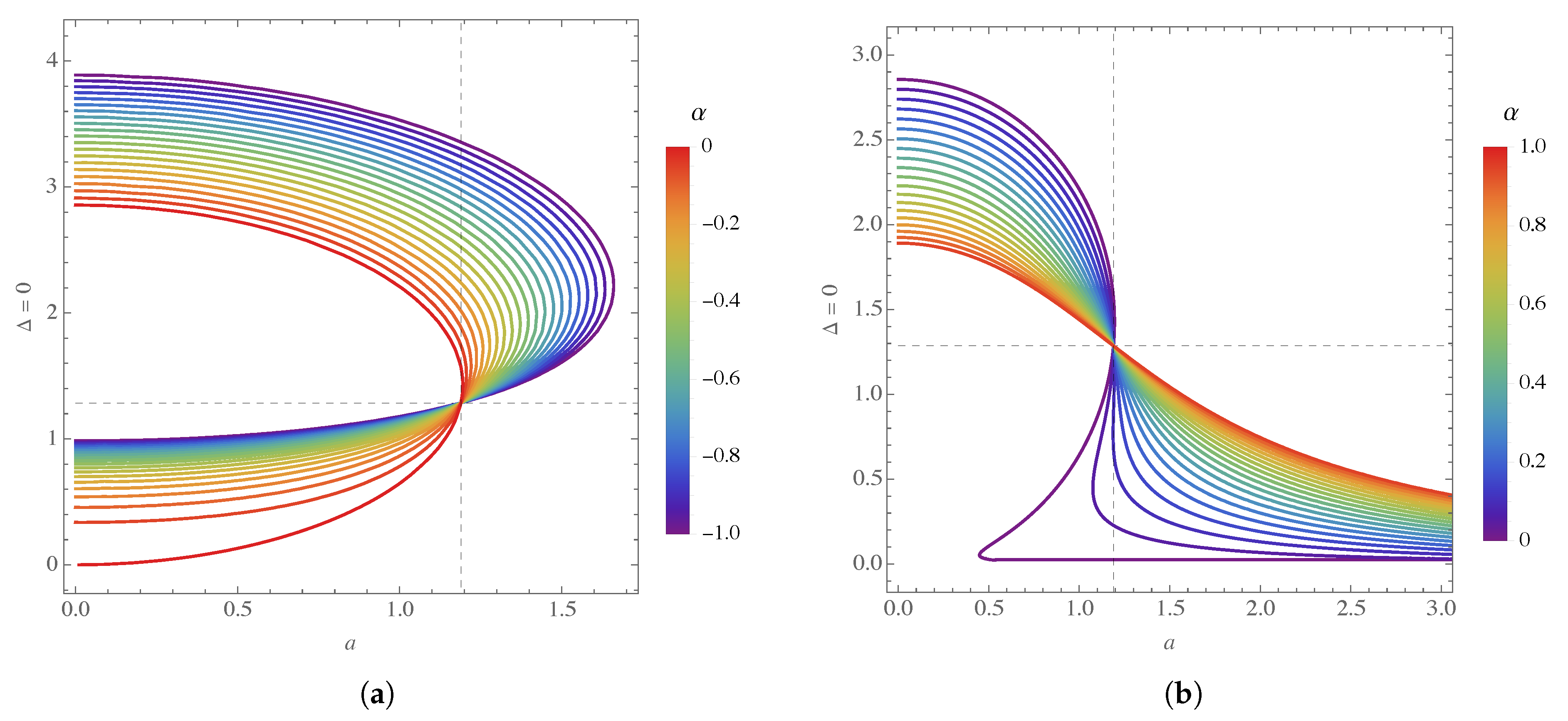
4. Horizons and the Causal Structure

The black hole horizons are identified by the polynomial equation $\Delta =0$, whose discriminant is given by

$$\begin{array}{c}{\mathcal{D}}_{\Delta }\equiv \mathrm{Disc}(\Delta =0)=-10976\left(1-\gamma \right){\gamma }^3{\alpha }^3+4\left[\left(81\left(26-27\gamma \right)\gamma +277\right)M^2-588\left(1-\gamma \right)a^2\right]{\gamma }^2{\alpha }^2\hfill \\ \hfill +\left[\left(95-81\gamma \right)a^2{M}^2-72M^4-21\left(1-\gamma \right)a^4\right]\gamma \alpha +4a^4{M}^2-4\left(1-\gamma \right)a^6.\end{array}$$

(39)

In Figure 2, the regions where ${\mathcal{D}}_{\Delta }\ge 0$ have been shown for both cases of $\alpha \le 0$ and $\alpha >0$. As can be observed from the diagrams, the case of $\alpha \le 0$ distinguishes between a black hole and a naked singularity through an extremal case where the two black hole horizons merge. On the other hand, for $\alpha >0$, we never encounter a naked singularity, as the black hole can have three horizons for certain values of $\alpha$. By merging two of these horizons, the black hole still retains an event horizon and a Cauchy horizon, which merge when ${\mathcal{D}}_{\Delta }=0$, leaving the black hole with only one horizon for all other corresponding values of $\alpha$. Note that the values of the spin parameter $a=a_{\mathrm{ext}}$, at which the horizons merge, can be obtained from the equation ${\mathcal{D}}_{\Delta }=0$, which yields

$$\begin{array}{ccc}\hfill a_{\mathrm{ext}}& =& {\displaystyle \frac{1}{\sqrt{6}}}\{{\displaystyle 〚}2\sqrt[3]{2}{M}^4+2M^2(486\sqrt[3]{2}\alpha {(1-\gamma )}^2\gamma -{{\displaystyle [}{a}_0-2M^6+2430\alpha {(1-\gamma )}^2\gamma M^4+59049{\alpha }^2{(1-\gamma )}^4{\gamma }^2{M}^2{\displaystyle ]}}^{1/3})\hfill \\ & & +{{\displaystyle (}2a_0-4M^6+4860\alpha {(1-\gamma )}^2\gamma M^4+118098{\alpha }^2{(1-\gamma )}^4{\gamma }^2{M}^2{\displaystyle )}}^{2/3}\hfill \\ & & -84\alpha (1-\gamma )\gamma {{\displaystyle (}{a}_0-2M^6+2430\alpha {(1-\gamma )}^2\gamma M^4+59049{\alpha }^2{(1-\gamma )}^4{\gamma }^2{M}^2{\displaystyle )}}^{1/3}{\displaystyle 〛}\hfill \\ & & \times 〚(1-\gamma ){{\displaystyle [}{a}_0-2M^6+2430\alpha {(1-\gamma )}^2\gamma M^4+59049{\alpha }^2{(1-\gamma )}^4{\gamma }^2{M}^2{\displaystyle ]}}^{1/3}{〛}^{-1}{{\displaystyle \}}}^{1/2},\hfill \end{array}$$

(40)

in which $a_0=9M^2\sqrt{3\alpha {(1-\gamma )}^2\gamma {\left[243\alpha {(1-\gamma )}^2\gamma -4M^2\right]}^3}$. For each fixed value of $\alpha$ and $\gamma$, if $a>{\alpha }_{\mathrm{ext}}$ holds, one can expect a naked singularity for $\alpha \le 0$, and a one-horizon black hole for $\alpha >0$. The conditions stated above can be observed in the behavior of the $\Delta$ function for fixed $\alpha$ and $\gamma$, as shown in Figure 3, where different values of the spin parameter have been taken into account. As we can observe, for $\alpha \le 0$, the equation $\Delta =0$ has two real positive roots when $a<a_{\mathrm{ext}}$ and one real positive root when $a=a_{\mathrm{ext}}$. For $a>a_{\mathrm{ext}}$, no real positive roots exist. In the case of $\alpha >0$, as inferred from Figure 2b, there are two distinct values for $a_{\mathrm{ext}}$, namely $a_{{\mathrm{ext}}_1}$ and $a_{{\mathrm{ext}}_2}$. When $a_{{\mathrm{ext}}_1}<a<a_{{\mathrm{ext}}_2}$, there are three real positive roots for $\Delta =0$, corresponding to a black hole with three horizons. At $a=a_{{\mathrm{ext}}_1}$ or $a=a_{{\mathrm{ext}}_2}$, two of these roots coalesce, leaving two positive roots. When $a<a_{{\mathrm{ext}}_1}$ or $a>a_{{\mathrm{ext}}_2}$, the two remaining roots also merge, resulting in a black hole with a single horizon. It is also informative to show, graphically, the behavior of the equation $\Delta =0$ within both scenarios of the $\alpha$ parameter. In Figure 4, we have plotted the profile of this equation for different values of the $\alpha$ parameter, regarding changes in the spin parameter, when $\gamma$ is fixed. It can be directly inferred from the diagrams that, for $\alpha \le 0$, the equation $\Delta =0$ has two real positive roots, which merge into a single point as the spin parameter increases, corresponding to the EBH. In contrast, for $\alpha >0$, the equation $\Delta =0$ yields three real positive roots for small values of the spin parameter. As the spin parameter increases, the number of real positive roots decreases, eventually leaving only one horizon for larger values of the spin parameter.

One can also calculate analytically the roots of $\Delta =0$, which give

$$\begin{array}{ccc}& & r_1={\displaystyle \frac{4}{1-\gamma }}\sqrt{{\displaystyle \frac{{\chi }_2}{3}}}\cos \left({\displaystyle \frac{1}{3}}\arccos \left({\displaystyle \frac{3{\chi }_3}{{\chi }_2}}\sqrt{{\displaystyle \frac{3}{{\chi }_2}}}\right)-{\displaystyle \frac{4\pi }{3}}\right)+{\displaystyle \frac{2M}{3(1-\gamma )}},\hfill \end{array}$$

(41)

$$\begin{array}{ccc}& & r_2={\displaystyle \frac{4}{1-\gamma }}\sqrt{{\displaystyle \frac{{\chi }_2}{3}}}\cos \left({\displaystyle \frac{1}{3}}\arccos \left({\displaystyle \frac{3{\chi }_3}{{\chi }_2}}\sqrt{{\displaystyle \frac{3}{{\chi }_2}}}\right)-{\displaystyle \frac{2\pi }{3}}\right)+{\displaystyle \frac{2M}{3(1-\gamma )}},\hfill \end{array}$$

(42)

$$\begin{array}{ccc}& & r_3={\displaystyle \frac{4}{1-\gamma }}\sqrt{{\displaystyle \frac{{\chi }_2}{3}}}\cos \left({\displaystyle \frac{1}{3}}\arccos \left({\displaystyle \frac{3{\chi }_3}{{\chi }_2}}\sqrt{{\displaystyle \frac{3}{{\chi }_2}}}\right)\right)+{\displaystyle \frac{2M}{3(1-\gamma )}},\hfill \end{array}$$

(43)

where

$$\begin{array}{ccc}& & {\chi }_2=-{\displaystyle \frac{1}{12}}\left[3a^2(1-\gamma )+42\alpha \gamma (1-\gamma )-4M^2\right],\hfill \end{array}$$

(44a)

$$\begin{array}{ccc}& & {\chi }_3=-{\displaystyle \frac{M}{216}}\left[9a^2(1-\gamma )-9\alpha \gamma \left(27{\gamma }^2-40\gamma +13\right)-8M^2\right].\hfill \end{array}$$

(44b)

Note that the correspondence of these roots to the black hole horizons depends strictly on the sign of the $\alpha$ parameter. For $\alpha \le 0$, when all roots are real, the black hole possesses a Cauchy and an event horizon, which are determined respectively by $r_{-}=r_2$ and $r_{+}=r_3$, with the other root being negative, i.e., $r_1<0$. As discussed before, the EBH occurs when $r_{-}=r_{+}$, beyond which a naked singularity arises. On the other hand, for $\alpha >0$, there exists an intermediate horizon $r_{-}=r_1<r_{\mathrm{in}}=r_2<r_{+}=r_3$ between the inner Cauchy horizon and the event horizon, when the conditions are favorable. This horizon disappears for $a=a_{{\mathrm{ext}}_{1,2}}$, and finally, $r_{-}$ also disappears when the above conditions are not satisfied, leaving a black hole with only one horizon $r_{+}$.

It is important to emphasize that, in addition to horizons, stationary black holes exhibit other hypersurfaces where static observers, whose world-lines are expressed as $\mathit{u}={(-g_{tt})}^{-1/2}{\mathbf{\xi }}^t$, cannot exist. Here, ${\mathbf{\xi }}^t$ represents the time-like Killing vector of the spacetime, aligned with the time coordinate. These hypersurfaces are known as static limits, where the observer’s four-velocity $\mathit{u}$ becomes null. The radii of these static limits, $r_{\mathrm{sl}}$, can be obtained by replacing $a\to a\cos \theta$ in the solutions (41)–(43). In this sense, we obtain two hypersurfaces defined by the radii $r_{{\mathrm{sl}}_{+}}$ and $r_{{\mathrm{sl}}_{-}}$, which constrain the regions where a static observer can exist. These surfaces obey the hierarchy $r_{{\mathrm{sl}}_{+}}\ge r_{+}\ge r_{-}\ge r_{{\mathrm{sl}}_{-}}$. Thus, the outer ergoregion is identified as $r_{+}\le r\le r_{{\mathrm{sl}}_{+}}$, while the inner ergoregion is identified by $r_{{\mathrm{sl}}_{-}}\le r\le r_{-}$. Within these regions, no static observer can exist. Considering the Cartesian coordinates $x=r\sin \theta \cos \varphi$, $y=r\sin \theta \sin \varphi$, and $z=r\cos \theta$, Figure 5 and Figure 6 demonstrate several examples of the ergoregions for negative and positive values of the $\alpha$ parameter, respectively. According to the diagrams, for $\alpha <0$, the interior ergoregions become more similar to those of the KBH as we reduce the $\gamma$ parameter. However, the extremality for the RMBH shows significant differences from that of a KBH. The same holds for the corresponding naked singularity. When $\alpha >0$, the significant differences are more apparent for the three-horizon black holes, as the interior ergosurface never forms inside the smallest horizon. Once again, by decreasing the value of $\gamma$, the spacetime mimics the exterior geometry of a KBH, which, in the examined cases, corresponds to a naked singularity. For the cases of $a<a_{{\mathrm{ext}}_1}$ and $a>a_{{\mathrm{ext}}_2}$, as demonstrated in Figure 3b, a one-horizon black hole is formed, which is small for the former case and significantly larger for the latter case.

Now that the spacetime structure of the RMBH has been studied in detail, beginning in the next section, we turn our attention to the parametrization of null geodesics in the exterior geometry of the black hole, which has been obtained within the MNJA, through the method of separation of the Hamilton–Jacobi equation.

5. Separation of the Hamilton–Jacobi Equation and Null Geodesics

It has been shown in Ref. [25] that the stationary spacetimes obtained from the NJA, in the case that they can be presented in Boyer–Lindquist-like coordinates, will also allow separability of the Hamilton–Jacobi equation. For the case of $A\left(r\right)=B\left(r\right)$, this separability has also been studied in Ref. [20] in the context of the MNJA, and for the case of $A\left(r\right)\ne B\left(r\right)$, this separability has been studied in Ref. [27]. There, the authors argue that although, due to the complexity of (38), it is a formidable task to determine a general solution for $\mathrm{\Psi }$ when $A\left(r\right)\ne B\left(r\right)$, this function, however, does not need to be identified explicitly in the study of null geodesics, since the separability of the Hamilton–Jacobi equation is independent of this function. In fact, the Hamilton–Jacobi equation is given by

$${\displaystyle \frac{\partial \mathcal{S}}{\partial \tau }}+\mathcal{H}=0,$$

(45)

in which $\mathcal{S}$ is the Jacobi action, $\tau$ is the affine parameter of the geodesic curves, and $\mathcal{H}$ is the canonical Hamiltonian, expressed as

$$\mathcal{H}={\displaystyle \frac{1}{2}}{g}^{\mu \nu }{p}_{\mu }{p}_{\nu },$$

(46)

with $\mathit{p}$ being the conjugate momentum covector, which is defined as

$$p_{\mu }={\displaystyle \frac{\partial \mathcal{S}}{\partial x^{\mu }}}.$$

(47)

In this manner, the constants of motion can be defined by exploiting the spacetime symmetries associated with the t and $\varphi$ coordinates. These constants are given by $E=-p_t$ and $L=p_{\varphi }$, where E represents the energy and L denotes the angular momentum of the test particles. Consequently, we can adopt the ansatz

$$\mathcal{S}={\displaystyle \frac{m^2}{2}}\tau -Et+L\varphi +{\mathcal{S}}_r\left(r\right)+{\mathcal{S}}_{\theta }\left(\theta \right),$$

(48)

for the Jacobi action, in which m is the test particles’ mass. By applying this ansatz, along with the definitions given in (46) and (47), and the line element in (37), the Hamilton–Jacobi Equation (45) yields

$$-{\displaystyle \frac{1}{\mathrm{\Psi }\Delta }}{\left[E\left(K+a^2\right)-aL\right]}^2+{\displaystyle \frac{p_{\theta }^2}{\mathrm{\Psi }}}+{\displaystyle \frac{1}{\mathrm{\Psi }{\sin }^2\theta }}{\left(aE{\sin }^2\theta -L\right)}^2+{\displaystyle \frac{\Delta p_r^2}{\mathrm{\Psi }}}=-m^2.$$

(49)

For null geodesics, it is naturally $m=0$, and hence, the conformal factor $\mathrm{\Psi }$ does not contribute. Accordingly, we can infer the equation

$$\Delta p_r^2-{\displaystyle \frac{1}{\Delta }}{\left[E\left(K+a^2\right)-aL\right]}^2=-\left[p_{\theta }^2+{\displaystyle \frac{1}{{\sin }^2\theta }}{\left(aE{\sin }^2\theta -L\right)}^2\right]\equiv \mathcal{K},$$

(50)

where we have separated the r-dependent segment of the equation from the $\theta$-dependent part, using a constant $\mathcal{K}$ defined as

$$\mathcal{K}=\mathcal{Q}+{\left(aE-L\right)}^2,$$

(51)

with $\mathcal{Q}$ representing Carter’s constant [44]. Based on this method, the equations for $p_r$ and $p_{\theta }$ are obtained as

$$\begin{array}{ccc}\hfill p_r^2& =& {\displaystyle \frac{1}{{\Delta }^2}}{\left[E\left(K+a^2\right)-aL\right]}^2-{\displaystyle \frac{1}{\Delta }}\left[\mathcal{Q}+{\left(aE-L\right)}^2\right],\hfill \end{array}$$

(52)

$$\begin{array}{ccc}\hfill p_{\theta }^2& =& \mathcal{Q}+a^2{E}^2{\cos }^2\theta -L^2{\cot }^2\theta .\hfill \end{array}$$

(53)

As we can see from the above equations, the Hamilton–Jacobi equation is fully separable for null geodesics in the line element (37). It is important to highlight that the NJA admits the separability of the Hamilton–Jacobi equations only if the rotating spacetime’s line element can be written in Boyer–Lindquist-like coordinates. In the context of the MNJA, however, this separability always holds for null geodesics. Now, since $p_{\mu }=g_{\mu \nu }{u}^{\nu }=g_{\mu \nu }\left(d{x}^{\nu }/d\tau \right)$, with the help of Equations (52) and (53), we can write the full set of equations of motion for null geodesics as follows:

$$\begin{array}{ccc}\hfill \mathrm{\Psi }{\displaystyle \frac{dt}{d\tau }}& =& {\displaystyle \frac{E}{\Delta }}[{\left(K+a^2\right)}^2-a^2\Delta {\sin }^2\theta -a\left(K+a^2-\Delta \right)\xi ],\hfill \end{array}$$

(54)

$$\begin{array}{ccc}\hfill \mathrm{\Psi }{\displaystyle \frac{dr}{d\tau }}& =& E\sqrt{\mathcal{R}\left(r\right)},\hfill \end{array}$$

(55)

$$\begin{array}{ccc}\hfill \mathrm{\Psi }{\displaystyle \frac{d\theta }{d\tau }}& =& E\sqrt{\Theta \left(\theta \right)},\hfill \end{array}$$

(56)

$$\begin{array}{ccc}\hfill \mathrm{\Psi }{\displaystyle \frac{d\varphi }{d\tau }}& =& {\displaystyle \frac{E}{\Delta {\sin }^2\theta }}[\left(\Delta -a^2{\sin }^2\theta \right)\xi +a{\sin }^2\theta \left(K+a^2-\Delta \right)],\hfill \end{array}$$

(57)

where

$$\begin{array}{ccc}\hfill \xi & =& {\displaystyle \frac{L}{E}},\hfill \end{array}$$

(58a)

$$\begin{array}{ccc}\hfill \eta & =& {\displaystyle \frac{\mathcal{Q}}{E^2}},\hfill \end{array}$$

(58b)

are the gauge-invariant constants of motion, and we have also defined

$$\begin{array}{ccc}\hfill \mathcal{R}\left(r\right)& =& {\left(K+a^2-a\xi \right)}^2-\Delta \left[\eta +{\left(a-\xi \right)}^2\right],\hfill \end{array}$$

(59a)

$$\begin{array}{ccc}\hfill \Theta \left(\theta \right)& =& \eta +{\cos }^2\theta \left(a^2-{\displaystyle \frac{{\xi }^2}{{\sin }^2\theta }}\right).\hfill \end{array}$$

(59b)

It is essential to rely on the conditions $R\left(r\right)\ge 0$ and $\Theta \left(\theta \right)\ge 0$ for the null trajectories to exist in the exterior geometry of the black hole.

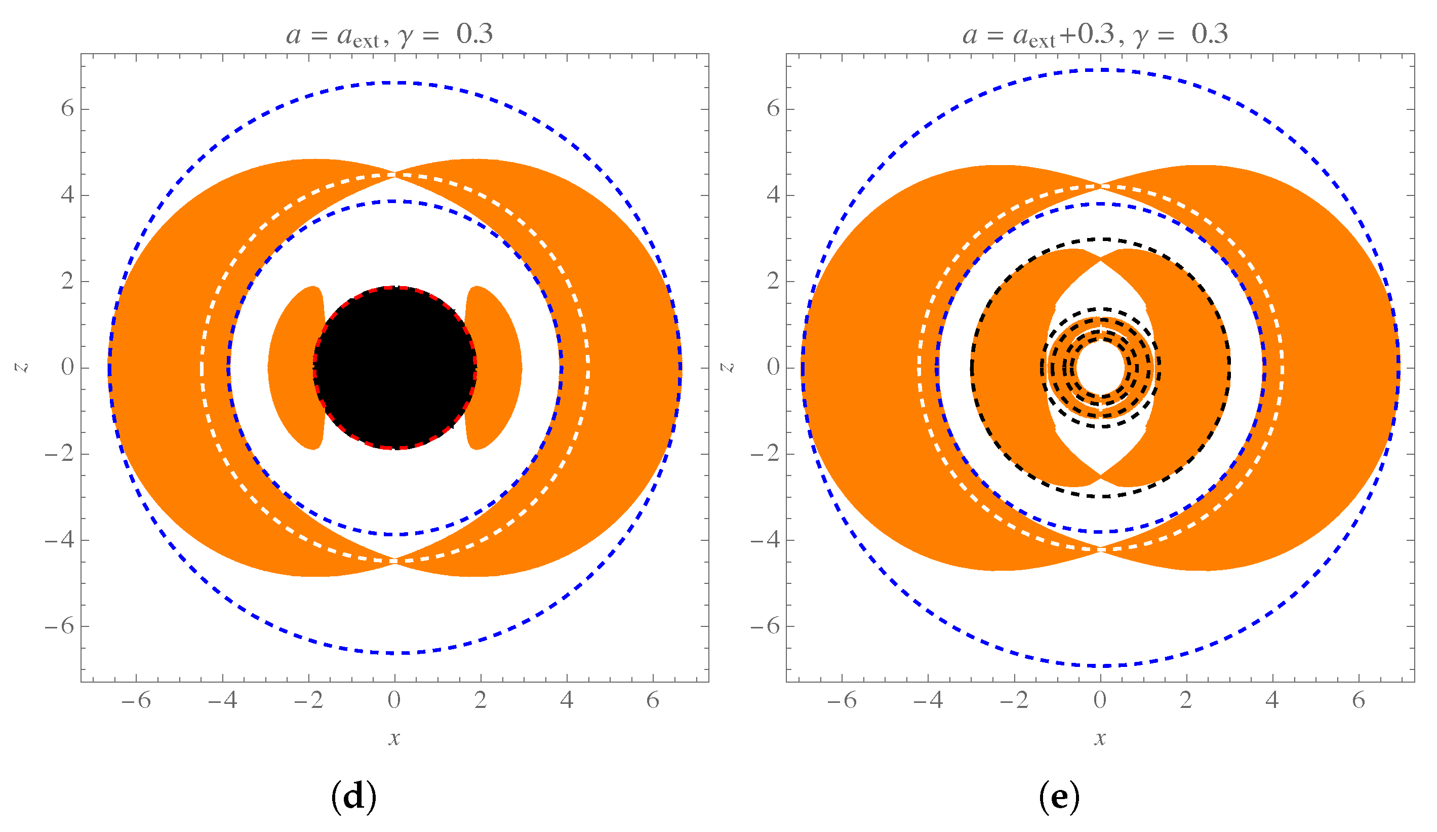
5.1. Orbits of Constant Radius and the Photon Regions

In curved spacetimes, understanding particle and photon trajectories involves analyzing their radial motion. For light rays, this analysis centers on the radial equation of motion, leading to different types of orbits, such as deflecting, captured, and spherical (critical) orbits. Spherical photon orbits, in particular, represent paths where the radial coordinate remains constant, skimming the black hole’s horizon. These orbits are critical because they determine whether a photon escapes or plunges into the black hole, and they are inherently unstable, forming an infinite sequence of photon rings that define the black hole’s shadow. In static spacetimes like Schwarzschild, these orbits are planar; however, in rotating black holes, frame-dragging creates a photon region where spherical orbits become non-planar. This region, bounded by the innermost and outermost circular orbits, defines the photon orbits, as extensively studied in KBH solutions (see Refs. [45,46,47]). Research on these orbits and their observational significance has expanded significantly in Kerr and Kerr-like spacetimes (see Refs. [40,48,49,50,51,52,53,54,55,56,57,58,59,60,61,62]).

In fact, spherical photon orbits at a given radius $r_p$ are determined under the criteria $\mathcal{R}\left(r_p\right)=0={\mathcal{R}}^{\prime }\left(r_p\right)$ [50]. Exploiting the form given in Equation (59a), these equations provide the sets of solutions

$$\begin{array}{ccc}& & {\xi }_p={\left({\displaystyle \frac{K+a^2}{a}}\right)}_{r_p},\hfill \end{array}$$

(60)

$$\begin{array}{ccc}& & {\eta }_p=-{\left({\displaystyle \frac{K^2}{a^2}}\right)}_{r_p},\hfill \end{array}$$

(61)

and

$$\begin{array}{ccc}& & {\xi }_p={\left({\displaystyle \frac{K+a^2}{a}}-{\displaystyle \frac{2K^{\prime }\Delta }{a{\Delta }^{\prime }}}\right)}_{r_p},\hfill \end{array}$$

(62)

$$\begin{array}{ccc}& & {\eta }_p={\left({\displaystyle \frac{4\Delta {\left(K^{\prime }\right)}^2}{{\left({\Delta }^{\prime }\right)}^2}}-{\displaystyle \frac{1}{a^2}}{\left[K-{\displaystyle \frac{2K^{\prime }\Delta }{{\Delta }^{\prime }}}\right]}^2\right)}_{r_p}.\hfill \end{array}$$

(63)

These equations determine the critical impact parameter for light rays on constant-r orbits. However, it is clear from Equation (61) that ${\eta }_p<0$, which leads to a non-physical result. Thus, we disregard the solutions in (60) and (61) and instead consider those in Equations (62) and (63) as the critical constants of motion for spherical photon orbits. Notably, for planar orbits with $\theta =\pi /2$, one can infer from Equations (56) and (59b) that ${\eta }_p=0$. This result allows us to use Equation (63) to obtain the radii of planar circular photon orbits. For the RMBH spacetime, given the complexity of the metric functions (4) and (5), this equation results in a polynomial of the fifteenth order, rendering the radii of planar photon orbits analytically intractable. However, numerical solutions can be used to determine the radii of prograde and retrograde planar circular orbits, $r_{p_{-}}$ and $r_{p_{+}}$, respectively, which define the inner and outer boundaries of the photon region. The photon region is characterized by the condition $\Theta \left(\theta \right)\ge 0$ for spherical photon orbits, using the critical impact parameters in Equations (62) and (63) in the angular potential (59b). By solving for the radii with ${\eta }_p=0$, we illustrate examples of the photon regions forming around the RMBH, as shown in Figure 7 and Figure 8, for various parameter values as exemplified in Figure 5 and Figure 6. In these diagrams, in addition to the radii of planar orbits $r_0$, we have also shown the radii of polar orbits, which indicate the spherical orbits for photons with no associated angular momentum. These photons traverse the entire polar angle, passing through the poles without any change in the azimuthal angle. The radii of such orbits are thus obtained by solving the equation ${\xi }_p=0$ using the expression in Equation (62). As observed from the diagrams, photon regions can form within $r_{p_{-}}$ for both cases, as these regions are bounded by the black hole’s event horizon. Notably, photon regions can also form inside the event horizon (see, for example, Ref. [52]), with these regions bounded by the radii of circular orbits within the black hole. When a naked singularity forms for $\alpha <0$, these regions replicate, generating photon regions of decreasing size as they approach the singularity. For black holes with $\alpha >0$, interesting features emerge, as the interior photon regions (those within $r_{p_{-}}$) vary in size and can form distinct branches, each containing a separate spherical polar orbit.

It is important to note that, for a distant observer, the photons residing within the photon regions (i.e., photons on spherical orbits) form the innermost photon rings, as they complete numerous half-orbits around the black hole before reaching the observer (for further discussion, see Refs. [63,64,65], as well as the foundational works in Refs. [66,67,68]). These photons thus play a key role in defining the true boundary of the shadow (or the critical curve), which will be explored in the next subsection.

5.2. The Black Hole Shadow

The study of light propagation around black holes holds significant importance in astrophysics, especially given the insights enabled by advances in observational astronomy. Photons on unstable orbits in the gravitational field of a black hole either fall onto the event horizon or escape to infinity. To a distant observer, those that escape appear as a bright photon ring that bounds the black hole shadow [46,69,70,71]. In particular, Luminet’s 1979 optical simulation of a SBH and its accretion [71] provided detailed insights into photon rings formed in the highly warped regions around black holes. These insights helped scientists refine the shadow of rotating black holes within their respective photon rings. Subsequently, mathematical techniques to determine the size and shape of a KBH’s shadow were developed by Bardeen [46,47], later expanded upon by Chandrasekhar [45], and further generalized (see Refs. [52,72,73,74,75,76]). These methods enabled rigorous analytical, numerical, and observational studies across various black hole spacetimes in general relativity and alternative theories of gravity [25,27,39,42,43,77,78,79,80,81,82,83,84,85,86,87,88,89,90,91,92,93,94,95,96,97,98,99,100,101,102,103,104,105,106]. As a result, black hole shadows have become essential in understanding light propagation near event horizons. Recent studies have also explored correlations between black hole shadow properties and fundamental parameters, including thermodynamic quantities [107,108].

Historically, various definitions have been proposed in the literature to describe the visual characteristics of black holes. Synge introduced the concept of the escape cone [69], while Zeldovich and Novikov referred to the cone of gravitational radiation capture [109]. Bardeen, Chandrasekhar, and Luminet further popularized terms like the optical appearance of black holes and black hole image, which are now widely used to describe how black holes appear visually [45,47,71,110]. The term black hole shadow, introduced by Falcke, Melia, and Agol [111], specifically refers to the dark region within the apparent boundary of the black hole, which is sometimes termed the photon ring [55,112] or the critical curve [113] (see Ref. [114] for further historical insights). In the context of the current study, the shadow is supposed to be bounded by the innermost light rings that represent lensed images of the luminous background.

Technically, in order to identify the shape of the black hole shadow, one might construct a celestial two-dimensional plane that spans the black hole’s image in the eyes of a distant observer. For the case of the RMBH, since the spacetime is asymptotically finite, it is convenient to identify the celestial plane by means of the celestial coordinates [73]

$$\begin{array}{ccc}& & X=\underset{r_o\to \infty }{\lim }\left(-r_o^2\sin {\theta }_o{\left.{\displaystyle \frac{\mathrm{d}\varphi }{\mathrm{d}r}}\right|}_{(r_o,{\theta }_o)}\right),\hfill \end{array}$$

(64)

$$\begin{array}{ccc}& & Y=\underset{r_o\to \infty }{\lim }\left(r_o^2{\left.{\displaystyle \frac{\mathrm{d}\theta }{\mathrm{d}r}}\right|}_{(r_o,{\theta }_o)}\right),\hfill \end{array}$$

(65)

for an observer located at the point $(r_o,{\theta }_o)$, where $r_o$ is the observer’s radial distance to the black hole, and ${\theta }_o$ is the observer’s inclination angle. Exploiting the equations of motion (55)–(57), one can derive the celestial coordinates for an observer at infinity. From the expressions (4) and (5), it is evident that at infinity $A\left(r_o\right)=B\left(r_o\right)=1-\gamma$, and hence, using the definitions (64) and (65), the celestial coordinates are obtained as

$$\begin{array}{ccc}& & X=-{\displaystyle \frac{{\xi }_p\left(r_p\right)}{\sin {\theta }_o}}-{\displaystyle \frac{a\gamma \sin {\theta }_o}{1-\gamma }},\hfill \end{array}$$

(66)

$$\begin{array}{ccc}& & Y=\pm \sqrt{{\eta }_p\left(r_p\right)+a^2{\cos }^2{\theta }_o-{\xi }_p^2\left(r_p\right){\cot }^2{\theta }_o},\hfill \end{array}$$

(67)

which, as expected, incorporates the conical parameter $\gamma$. Obviously, for $\gamma =0$, the above coordinates resemble those for asymptotically flat spacetime (such as for KBH) given in Ref. [45]. To demonstrate the critical curves, it is also convenient to locate the observer on the equatorial plane by setting ${\theta }_o=\pi /2$, and hence, the celestial coordinates that will be used for plotting the shadow boundaries take the form

$$\begin{array}{ccc}& & X=-{\xi }_p\left(r_p\right)-{\displaystyle \frac{a\gamma }{1-\gamma }},\hfill \end{array}$$

(68)

$$\begin{array}{ccc}& & Y=\pm \sqrt{{\eta }_p\left(r_p\right)}.\hfill \end{array}$$

(69)

Note that at each point on the critical curve in the celestial plane, one can consider a circle centered at the origin, whose radius $R_c$ can be calculated by using the expressions in Equations (62) and (63) in the celestial coordinates (66) and (67), which yields

$$\begin{array}{ccc}\hfill R_c^2& =& X^2+Y^2\hfill \\ & =& {\displaystyle \frac{1}{2{(1-\gamma )}^2}}{\left[a^2\left(3-2\gamma +\left(1-2\gamma \right)\cos \left(2{\theta }_o\right)\right)+4\left(1-\gamma \right)K-{\displaystyle \frac{8\left(1-\gamma \right)K^{\prime }\Delta \left({\Delta }^{\prime }-\left(1-\gamma \right)K^{\prime }\right)}{{\left({\Delta }^{\prime }\right)}^2}}\right]}_{r_p}.\hfill \end{array}$$

(70)

Now, considering the critical constants in Equations (62) and (63), we take $r_p$ as the curve parameter and generate the shadow boundaries in the X–Y plane. In Figure 9, several examples of the critical curves have been plotted for the RMBH with different spin parameters, while the parameters $\alpha$ and $\gamma$ are also considered to be varying in some examples. As indicated by the diagrams, for a fixed value of $\alpha$, increasing the $\gamma$ parameter significantly enlarges the shadow compared to that of a KBH. Notably, for positive values of $\alpha$, the critical curves can resemble those of a Kerr naked singularity; however, here they correspond to RMBHs with either one or two horizons rather than to naked singularities. This is a distinctive feature of the RMBH spacetime, suggesting that high-spin RMBHs may manifest through unclosed photon rings. In these cases, photon regions do not form in the conventional sense, implying that the constants of motion $\xi$ and $\eta$, as given by Equations (58a) and (58b), do not permit a peak in the gravitational effective potential for photons approaching from all distances. Consequently, for certain black hole parameter values, the number of spherical photon orbits is reduced, with no solutions for $r_p$ under these conditions. In such scenarios, the majority of photons are either deflected toward an observer at infinity, forming alternative photon rings, or are deflected onto the event horizon and captured. Thus, the unclosed shadow boundaries correspond to a small subset of innermost unstable photon trajectories that reside on spherical orbits. Although previous studies have demonstrated that the shadows of KBHs and Kerr naked singularities may be indistinguishable to distant observers, it has also been shown that photon rings for black holes and naked singularities can exhibit observational differences [67,115,116,117,118,119]. For the RMBH, however, as inferred from the critical curves, unclosed photon rings do not necessarily correspond to naked singularities. This is further evident from the shadow diagrams for positive values of $\alpha$, which confirm that no naked singularities are present in the spacetime.

6. Shadow Observables and Constraints from the EHT

In this section, we begin by characterizing the shape of the black hole shadow through key observables, which we then apply to the RMBH to analyze the behavior of these observables specific to this black hole. Finally, we use these observables as tools to compare with EHT data to constrain the black hole parameters.

Recently, numerous studies have explored the deformation and distortion of black hole shadows (see, for instance, Refs. [87,98,112,120,121,122,123,124,125]). Following these approaches, the shadow can be characterized by the following features:

(i)

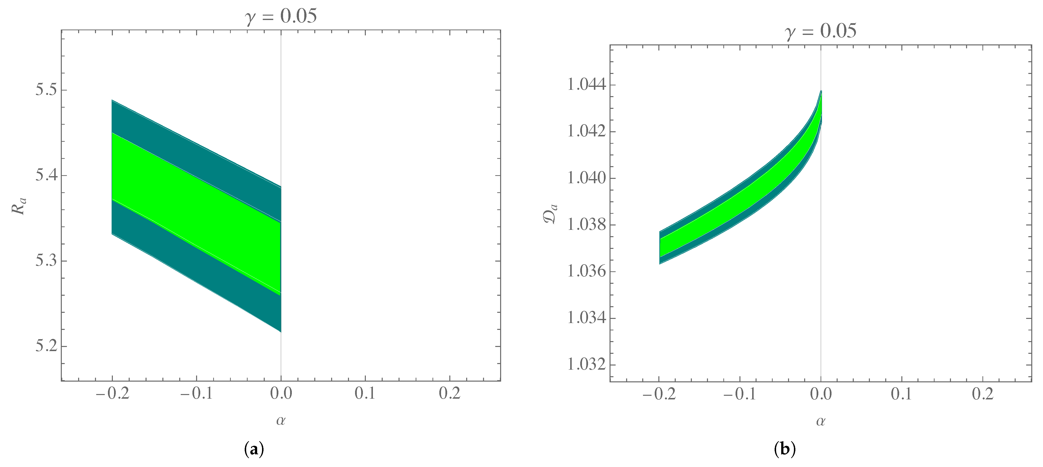
The areal radius $R_a$, which quantifies the size of the black hole shadow, is defined as

$$\begin{array}{ccc}& & R_a=\sqrt{{\displaystyle \frac{{\mathcal{A}}_s}{\pi }}},\hfill \end{array}$$

(71)

in which ${\mathcal{A}}_s$ is the area enclosed by the critical curve, given by

$${\mathcal{A}}_s=2\int Y\left(r\right)\mathrm{d}X\left(r\right)=2{\int }_{r_{p_{-}}}^{r_{p_{+}}}Y\left(r\right)X^{\prime }\left(r\right)\mathrm{d}r,$$

(72)

where the radii of planar orbits $r_{p_{\pm }}$ are determined from the equation $Y^2\left(r_p\right)=0$.

(ii)

The shadow deformation ${\mathcal{D}}_s$, which describes the shadow’s asymmetry, is given by

$${\mathcal{D}}_s={\displaystyle \frac{\delta Y}{\delta X}}={\displaystyle \frac{Y_t-Y_b}{X_r-X_l}}={\displaystyle \frac{2Y_t}{X_r-X_l}},$$

(73)

where the subscripts t, b, l, and r denote the top, bottom, left, and right extremities of the shadow, as illustrated in Figure 10, which depicts the geometric form of an oblate shadow.

For simplicity, we assume $Y_b=-Y_t$, justifying the factor of 2 in Equation (72) due to the shadow’s reflectional symmetry along the X-axis.

(iii)

The fractional deviation parameter ${\delta }_s$, which measures the deviation of the shadow’s diameter from that of the SBH, is defined as

$${\delta }_s={\displaystyle \frac{{\overline{R}}_{\mathrm{sh}}}{3\sqrt{3}}}-1,$$

(74)

where

$${\overline{R}}_{\mathrm{sh}}^2={\displaystyle \frac{1}{2\pi }}{\int }_0^{2\pi }\left[{\left(X-X_c\right)}^2+{\left(Y-Y_c\right)}^2\right]\mathrm{d}\psi ,$$

(75)

represents the average radius of the shadow, with $(X_c,Y_c=0)$ locating the geometric center of the shadow, where $X_c=(X_r+X_l)/2$. Additionally,

$$\psi =arctan\left({\displaystyle \frac{Y}{X-X_c}}\right),$$

(76)

is the angular position of points on the shadow boundary relative to the center.

Note that $X_r$ and $X_l$ are identified as $X\left(r_{p_{\pm }}\right)$, while the top end $Y_t$ corresponds to $Y\left(r_t\right)$, where $r_t$ is determined from the condition $\mathrm{d}Y/\mathrm{d}X=0$. Considering the celestial coordinates in Equations (66) and (67), along with the expressions in (62) and (63), the latter condition leads to the equation

$$2\left(a^2{s}_o^2-\Delta \right)K^{\prime }+\left[a^2\left(1-s_o^2\right)+K\right]{\Delta }^{\prime }=0,$$

(77)

where $s_o\equiv \sin {\theta }_o$. In Figure 11, we present the behavior of the areal radius, the deformation, and the deviation as functions of the $\alpha$ parameter for two different inclination angles.

Note that the discontinuous curves in the diagrams correspond to the discontinuous photon rings (as illustrated in some examples in Figure 9). In these cases, the celestial coordinates X and Y cannot be computed as real quantities, typically because the light rays fail to orbit stably around the black hole (see the discussion in the previous section). As observed from the diagrams in Figure 11a,d for each fixed $\gamma$-parameter, the areal radius smoothly decreases within its continuous value domain as the $\alpha$-parameter increases. Furthermore, an increase in the spin parameter leads to a reduction in the areal radius, which is consistent with the expected behavior for classical Kerr-like black holes in GR. Conversely, for a fixed $\gamma$-parameter, an increase in the $\alpha$-parameter results in a rise in the deformation, with a larger deformation for faster-rotating black holes. By comparing panels (b) and (e) of Figure 11, we can observe that for the same parameter values, a higher inclination angle leads to an increase in the deformation. Finally, as shown in Figure 11c,f, the deviation parameter is always positive, indicating that the average shadow radius of the RMBH is larger than that of the SBH and decreases rapidly as the $\alpha$-parameter increases. However, the positivity of ${\delta }_s$ also implies that as the spin parameter increases, the deviation diminishes. This trend is evident in the diagrams for both inclination angles and is in agreement with the behavior of the areal radius demonstrated in Figure 11a,d.

6.1. Constraints from the M87* Observations

The EHT observational results from the shadow images of M87* revealed the areal radius and deformation of the shadow, respectively, as $4.31M\le R_a\le 6.08M$ and $1\le {\mathcal{D}}_s\le 1.33$ [1]. Furthermore, it has been shown that the spin parameter of M87* is approximately $a=(0.9\pm 0.05)M$ [126]. Following the discussion in Ref. [127], we assume ${\theta }_o={17}^{\circ }$. Considering the spin parameter of M87* mentioned above, we observe from Figure 11a,b that the values of $R_a$ for the corresponding curve do not lie within the range observed for M87*. This suggests that the $\gamma$-parameter should be smaller. In Figure 12a, we have plotted the areal radius and the deformation as functions of $\alpha$ for the spin parameter of M87* within its $1\sigma$ and $2\sigma$ uncertainties, where the $\gamma$ parameter has been fixed to $0.05$.

As observed from the behavior of $R_a$, the value $\gamma =0.05$ places the domain of confidence within an acceptable range regarding the M87* observations. However, considering the range of $R_a$ covered within the $2\sigma$ uncertainty, it can be concluded that this parameter will still lie within the confident domain of M87* observations if the chosen value of $\gamma$ is doubled. Thus, we infer that the $\gamma$ parameter performs best within the range $0\le \gamma \lesssim 0.1$. Furthermore, the physically reliable range of $\alpha$ within these data is $-0.2\lesssim \alpha \le 0$, which can also be regarded as its observational constraint. Therefore, the negative branch of $\alpha$ holds more astrophysical significance. These constraints have been tested for the deformation in Figure 12b. Note that the range of ${\mathcal{D}}_s$ in diagrams Figure 11b,e for $\gamma =0.3$ is already within the acceptable ranges, particularly for $a=0.9M$. However, we see that for $\gamma =0.05$, the results are still acceptable. Hence, we can confidently adopt the new domain for $\gamma$ as asserted above, since it respects the validity of $R_a$ within the observational data.

6.2. Constraints from the Sgr A* Observations

The parameters of Sgr A* observed by the EHT are specified by the Very Large Telescope Interferometer (VLTI) and Keck observatories. These observations have constrained the areal radius and the fractional deviation peculiar to Sgr A* as $4.5M\le R_a\le 5.5M$ and $-0.17\le {\delta }_s\le 0.01$ by VLTI, and $4.3M\le R_a\le 5.3M$ and $-0.14\le {\delta }_s\le 0.05$ by Keck [2]. Furthermore, the inclination angle determined by the EHT was approximately ${\theta }_o<{50}^{\circ }$ for two classes of models used in simulations. For this purpose, two different spin parameters, $a=0.5M$ and $a=0.94M$, were applied to satisfy a series of EHT constraints in the general relativistic magnetohydrodynamic (GRMHD) simulations. On the other hand, recent analysis of Sgr A* suggests that its spin should be $a=(0.9\pm 0.06)M$ [127]. This value is taken into account in this subsection to constrain the parameters of the RMBH. Additionally, a reliable inclination of ${30}^{\circ }$ is assumed. In Figure 13, we have plotted the behavior of $R_a$ and ${\delta }_s$ for the RMBH, considering the spin parameter of Sgr A* within its $1\sigma$ and $2\sigma$ uncertainties.

As inferred from the left panel, the values of the areal radius lie within the observational data derived from VLTI and Keck, with $\gamma =0.05$ as the upper limit. This indicates that larger values of $\gamma$ would violate the observational constraints. Therefore, this suggests that, while the $\alpha$ parameter can still respect the domain $-0.2\lesssim \alpha \le 0$, the $\gamma$ parameter should be less than 0.05. This is also consistent with the behavior of ${\delta }_s$ within Sgr A* observations, as for the chosen value of $\gamma =0.036$, the fractional deviation becomes ${\delta }_s\approx 0.05$, which is the upper limit of this parameter according to the Keck observations. Hence, to be consistent with the Sgr A* observations, the $\gamma$ parameter should lie within the domain $0\le \gamma \lesssim 0.036$. Notably, this range just covers a portion of the acceptable values constrained by the M87* observational data. Thus, we can infer that the Sgr A* observations impose more stringent constraints on the parameters of the RMBH.

Based on these constraints, in Figure 14, we have plotted the shadow of the RMBH, considering the values for the $\alpha$ and $\gamma$ parameters that are in agreement with both the M87* and Sgr A* observations, as discussed above.

As we can see, within the observational constraints, the shadow radius of the RMBH is slightly larger than that of a KBH. Furthermore, in contrast to the oblateness of the shadow of a fast-rotating KBH, the shadow of a fast-rotating RMBH exhibits sharpness. This is an important feature of the weakly coupled GMC in the spacetime of the RMBH, which manifests itself in the peculiar shape of the shadow.

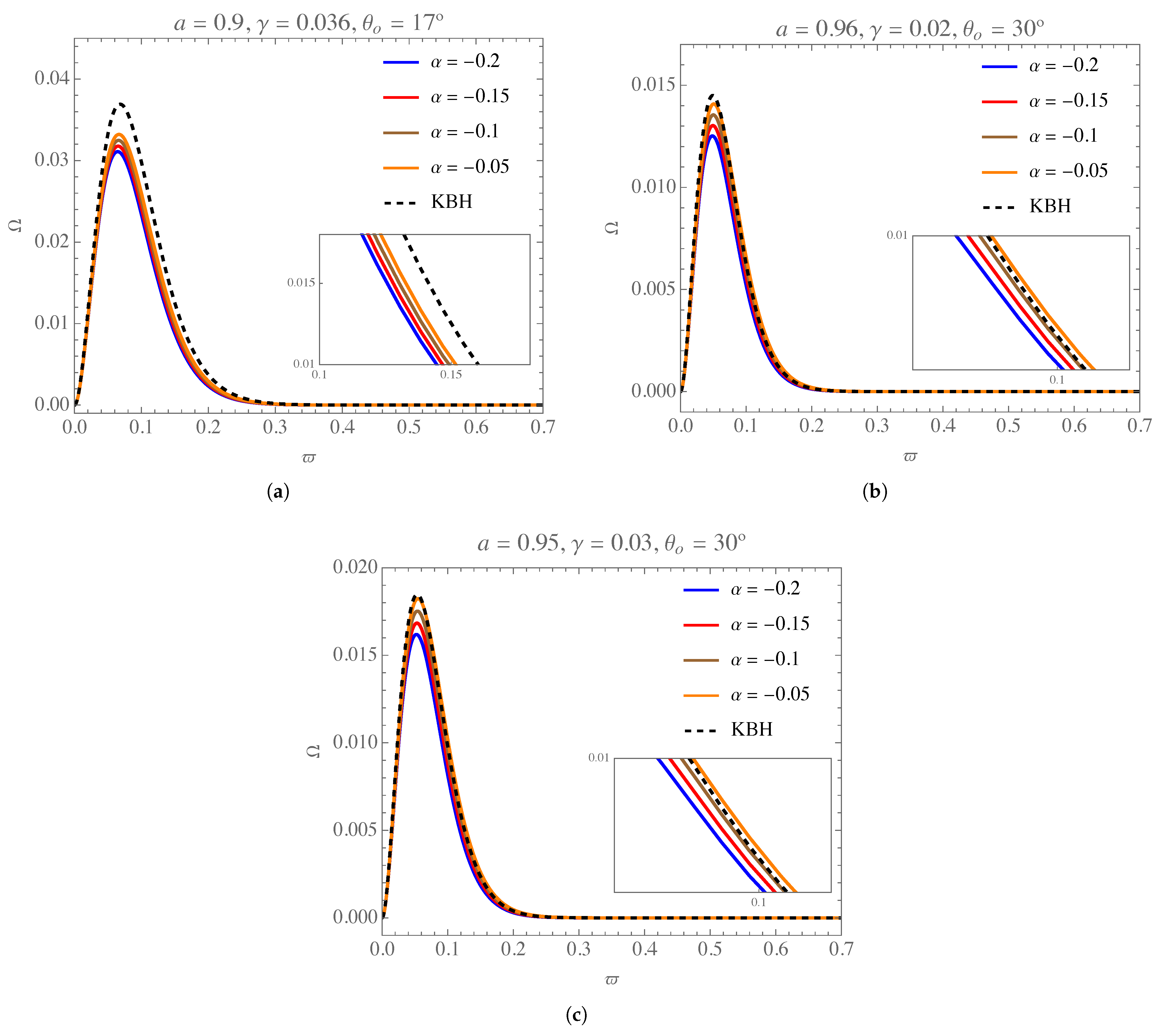
7. The Energy Emission Rate

From the quantum mechanical perspective, on the black hole’s event horizon, particles can be created and annihilated, and those with positive energy can escape the event horizon by tunneling. This process sets black holes into radiation, which may eventually cause them to evaporate. Black hole evaporation occurs due to Hawking radiation, a quantum effect in which black holes emit thermal radiation, gradually losing mass and energy over time until they eventually vanish [128]. At high energy levels, Hawking radiation is typically emitted within a finite cross-sectional area, denoted as ${\sigma }_l$. For distant observers positioned far from the black hole, this cross-section gradually approaches the shadow cast by the black hole [129,130]. It has been shown that ${\sigma }_l$ is directly linked to the area of the photon ring and can be mathematically represented as [130,131,132]

$${\sigma }_l\approx \pi {\overline{R}}_{\mathrm{sh}}^2.$$

(78)

Accordingly, the energy emission rate of the black hole can be expressed as

$$\Omega \equiv {\displaystyle \frac{{\mathrm{d}}^{2}E\left(\varpi \right)}{\mathrm{d}\varpi \mathrm{d}t}}={\displaystyle \frac{2{\pi }^2{\sigma }_l}{e^{\varpi /T_{\mathrm{H}}^{+}}-1}}{\varpi }^3\approx {\displaystyle \frac{2{\pi }^3{\overline{R}}_{\mathrm{sh}}^2{\varpi }^3}{e^{\varpi /T_{\mathrm{H}}^{+}}-1}},$$

(79)

where $\varpi$ is the emission frequency, and $T_{\mathrm{H}}^{+}=\kappa /2\pi$ is the Hawking temperature at the event horizon, where

$$\kappa ={\left.{\displaystyle \frac{{\Delta }^{\prime }\left(r\right)}{2\left(a^2+r^2\right)}}\right|}_{r_{+}},$$

(80)

is the surface gravity at the event horizon. It is straightforward to verify that for a zero spin parameter (i.e., $a=0$), this quantity reduces to $\kappa =A^{\prime }\left(r_{+}\right)/2$, which is the surface gravity of the event horizon for static black holes. In Figure 15, some examples of the behavior of $\Omega$ versus changes in the frequency $\varpi$ are plotted for the RMBH, with black hole parameters taken within the observationally accepted domains, as identified in the previous section. As observed from the diagrams, the larger the $\gamma$ parameter, the higher the energy emission rate for all values of the coupling constant $\alpha$. Hence, the GMC results in a faster-evaporating black hole. It is also observed that faster-rotating black holes emit less energy. Consequently, for higher spin parameters, the profiles of the RMBH resemble those of the KBH. Furthermore, as the observer’s inclination increases, the energy emission rate decreases. According to the diagrams, we can infer that the largest emission rate for the RMBH corresponds to the lower limit of the spin parameter, the upper limit of the coupling constant, and the upper limit of the GMC. However, note that such cases exhibit significantly lower energy emission rates than the KBH.

8. Summary and Conclusions

In this study, we analyzed the shadow properties of a rotating black hole with a weakly coupled GMC, i.e., the RMBH, which is derived by applying MNJA from the seed static spacetime. We showed that the GMC, by creating a deficit angle, modifies the black hole’s causal structure, photon regions, and shadow observables, while general relativity remains the background theory. Our findings reveal that the combined influence of the GMC and rotation produces distinct shadow features, which could potentially differentiate the RMBH from the Kerr-like black holes of GR. Our shadow analysis demonstrated how both the GMC and the weak coupling constant modify the size, circularity, and shape of the shadow, resulting in deviations that may be detectable in astrophysical observations. The investigation of critical curves in the shadow showed that, for specific values of the GMC and coupling parameters, certain photon trajectories remain open, especially under high-spin conditions. These open photon rings indicate incomplete spherical photon orbits, forming unique shadow boundaries for rotating black holes with GMC. Such characteristics may provide observable signatures that help distinguish the RMBH from the KBH. Moreover, using shadow observables, including the areal radius $R_a$ and the shadow deformation parameter ${\mathcal{D}}_s$, we constrained the GMC parameter $\gamma$ and weak coupling constant $\alpha$ by comparing theoretical shadow predictions with observational data from the EHT for M87* and Sgr A*. This analysis restricted the GMC parameter to $0\le \gamma \lesssim 0.036$ and the weak coupling constant to $-0.2\lesssim \alpha \le 0$. These constraints provide important experimental limits on the parameter space for black holes with GMC, offering insights into the symmetry-breaking scale associated with global monopoles in astrophysical scenarios. We further examined the black hole’s energy emission rate, observing that higher values of the GMC correspond to increased emission rates, suggesting a faster evaporation process. Our analysis indicates that emission rates are inversely related to the spin parameter, with higher rotation leading to a reduced emission rate. Additionally, observers at larger inclination angles experience decreased emission rates, suggesting that inclination angle and rotation significantly influence the black hole’s energy profile. In conclusion, our study underscores the potential of black hole shadow observations as a tool for testing nonminimal coupling theories and detecting topological defects like global monopoles. By constraining the GMC and coupling parameter, our results also provide a potential phenomenological test for nonminimal gravity. Future research may extend this analysis by exploring additional shadow observables, such as asymmetry or lensing rings, or by examining the behavior of GMC in stronger coupling regimes. Such investigations could further clarify the role of symmetry-breaking mechanisms and topological defects in shaping black hole spacetimes, providing valuable insights into modified gravity and early-universe physics.

References

- Akiyama, K.; et al.; [Event Horizon Telescope Collaboration] First M87 Event Horizon Telescope Results. I. The Shadow of the Supermassive Black Hole. Astrophys. J. 2019, 875, L1. [Google Scholar] [CrossRef]
- Akiyama, K.; et al.; [Event Horizon Telescope Collaboration] First Sagittarius A* Event Horizon Telescope results. I. The shadow of the supermassive black hole in the center of the Milky Way. Astrophys. J. Lett. 2022, 930, L12. [Google Scholar] [CrossRef]
- Vilenkin, A. Cosmic strings and domain walls. Phys. Rept. 1985, 121, 263–315. [Google Scholar] [CrossRef]
- Barriola, M.; Vilenkin, A. Gravitational field of a global monopole. Phys. Rev. Lett. 1989, 63, 341–343. [Google Scholar] [CrossRef]
- Achucarro, A.; Gregory, R. Turning inside out the AdS/CFT correspondence. Phys. Rev. Lett. 1999, 83, 1046–1049. [Google Scholar] [CrossRef]
- Nucamendi, U.; Salgado, M. Scalar hairy black holes and solitons in asymptotically flat space-times. Phys. Rev. D 2001, 63, 125016. [Google Scholar] [CrossRef]
- Kibble, T.W.B. Topology of cosmic domains and strings. J. Phys. A Math. Gen. 1976, 9, 1387. [Google Scholar] [CrossRef]
- Vilenkin, A.; Shellard, E. Cosmic Strings and Other Topological Defects; Cambridge Monographs on Mathematical Physics, Cambridge University Press: Cambridge, UK, 1994. [Google Scholar]
- Barros, A.; Romero, C. Global monopoles in Brans-Dicke theory of gravity. Phys. Rev. D 1997, 56, 6688–6691. [Google Scholar] [CrossRef]
- Liu, D.J.; Zhang, Y.L.; Li, X.Z. A self-gravitating Dirac–Born–Infeld global monopole. Eur. Phys. J. C 2009, 60, 495–500. [Google Scholar] [CrossRef]
- Caramês, T.R.P.; Bezerra de Mello, E.R.; Guimarães, M.E.X. Gravitational Field of a Global Monopole in a Modified Gravity. Int. J. Mod. Phys. Conf. Ser. 2011, 3, 446–454. [Google Scholar] [CrossRef]
- Caramês, T.R.P.; Fabris, J.C.; Bezerra de Mello, E.R.; Belich, H. f(R) global monopole revisited. Eur. Phys. J. C 2017, 77, 496. [Google Scholar] [CrossRef]
- Lambaga, R.D.; Ramadhan, H.S. Gravitational field of global monopole within the Eddington-inspired Born-Infeld theory of gravity. Eur. Phys. J. C 2018, 78, 436. [Google Scholar] [CrossRef]
- Nascimento, J.R.; Olmo, G.J.; Porfírio, P.J.; Petrov, A.Y.; Soares, A.R. Global monopole in Palatini f(R) gravity. Phys. Rev. D 2019, 99, 064053. [Google Scholar] [CrossRef]
- Gußmann, A. Scattering of axial gravitational wave pulses by monopole black holes and QNMs: A semianalytic approach. Class. Quantum Gravity 2021, 38, 035008. [Google Scholar] [CrossRef]
- Chatzifotis, N.; Mavromatos, N.E.; Theodosopoulos, D.P. Global monopoles in the extended Gauss-Bonnet gravity. Phys. Rev. D 2023, 107, 085014. [Google Scholar] [CrossRef]
- Caramês, T.R.P. Nonminimal global monopole. Phys. Rev. D 2023, 108, 084002. [Google Scholar] [CrossRef]
- Fathi, M.; Villanueva, J.; Caramês, T.R.; Morales-Díaz, A. Null geodesics around a black hole with weakly coupled global monopole charge. Ann. Phys. 2025, 472, 169863. [Google Scholar] [CrossRef]
- Newman, E.T.; Janis, A.I. Note on the Kerr Spinning-Particle Metric. J. Math. Phys. 1965, 6, 915–917. [Google Scholar] [CrossRef]
- Azreg-Aïnou, M. Generating rotating regular black hole solutions without complexification. Phys. Rev. 2014, D90, 064041. [Google Scholar] [CrossRef]
- Azreg-Aïnou, M. From static to rotating to conformal static solutions: Rotating imperfect fluid wormholes with(out) electric or magnetic field. Eur. Phys. J. C 2014, 74, 2865. [Google Scholar] [CrossRef]
- Bertolami, O.; Böhmer, C.G.; Harko, T.; Lobo, F.S.N. Extra force in f(R) modified theories of gravity. Phys. Rev. D 2007, 75, 104016. [Google Scholar] [CrossRef]
- Fisher, S.B.; Carlson, E.D. Nuclear limits on nonminimally coupled gravity. Phys. Rev. D 2022, 105, 024020. [Google Scholar] [CrossRef]
- March, R.; Bertolami, O.; Muccino, M.; Gomes, C.; Dell’Agnello, S. Cassini and extra force constraints to nonminimally coupled gravity with a screening mechanism. Phys. Rev. D 2022, 105, 044048. [Google Scholar] [CrossRef]
- Shaikh, R. Black hole shadow in a general rotating spacetime obtained through Newman-Janis algorithm. Phys. Rev. D 2019, 100, 024028. [Google Scholar] [CrossRef]
- Rodrigues, M.E.; Junior, E.L.B. Comment on “Generic rotating regular black holes in general relativity coupled to nonlinear electrodynamics”. Phys. Rev. D 2017, 96, 128502. [Google Scholar] [CrossRef]
- Junior, H.C.D.L.; Crispino, L.C.B.; Cunha, P.V.P.; Herdeiro, C.A.R. Spinning black holes with a separable Hamilton–Jacobi equation from a modified Newman–Janis algorithm. Eur. Phys. J. C 2020, 80, 1036. [Google Scholar] [CrossRef]
- Xu, Z.; Wang, J. Kerr-Newman-AdS black hole in quintessential dark energy. Phys. Rev. D 2017, 95, 064015. [Google Scholar] [CrossRef]
- Toshmatov, B.; Stuchlík, Z.; Ahmedov, B. Rotating black hole solutions with quintessential energy. Eur. Phys. J. Plus 2017, 132, 98. [Google Scholar] [CrossRef]
- Toshmatov, B.; Stuchlík, Z.; Ahmedov, B. Generic rotating regular black holes in general relativity coupled to nonlinear electrodynamics. Phys. Rev. D 2017, 95, 084037. [Google Scholar] [CrossRef]
- Kumar, R.; Ghosh, S.G. Rotating black hole in Rastall theory. Eur. Phys. J. C 2018, 78, 750. [Google Scholar] [CrossRef]
- Azreg-Aïnou, M.; Haroon, S.; Jamil, M.; Rizwan, M. Rotating normal and phantom Einstein–Maxwell–dilaton black holes: Geodesic analysis. Int. J. Mod. Phys. D 2019, 28, 1950063. [Google Scholar] [CrossRef]
- Contreras, E.; Ramirez–Velasquez, J.M.; Rincón, A.; Panotopoulos, G.; Bargueño, P. Black hole shadow of a rotating polytropic black hole by the Newman–Janis algorithm without complexification. Eur. Phys. J. C 2019, 79, 802. [Google Scholar] [CrossRef]
- Haroon, S.; Jusufi, K.; Jamil, M. Shadow Images of a Rotating Dyonic Black Hole with a Global Monopole Surrounded by Perfect Fluid. Universe 2020, 6, 23. [Google Scholar] [CrossRef]
- Kumar, R.; Ghosh, S.G. Rotating black holes in 4 D Einstein-Gauss Gravity Its Shad. J. Cosmol. Astropart. Phys. 2020, 2020, 053. [Google Scholar] [CrossRef]
- Contreras, E.; Rincón, A.; Panotopoulos, G.; Bargueño, P.; Koch, B. Black hole shadow of a rotating scale-dependent black hole. Phys. Rev. D 2020, 101, 064053. [Google Scholar] [CrossRef]
- Jusufi, K.; Jamil, M.; Chakrabarty, H.; Wu, Q.; Bambi, C.; Wang, A. Rotating regular black holes in conformal massive gravity. Phys. Rev. D 2020, 101, 044035. [Google Scholar] [CrossRef]
- Liu, C.; Zhu, T.; Wu, Q.; Jusufi, K.; Jamil, M.; Azreg-Aïnou, M.; Wang, A. Shadow and quasinormal modes of a rotating loop quantum black hole. Phys. Rev. D 2020, 101, 084001. [Google Scholar] [CrossRef]
- Fathi, M.; Olivares, M.; Villanueva, J.R. Ergosphere, Photon Region Structure, and the Shadow of a Rotating Charged Weyl Black Hole. Galaxies 2021, 9, 43. [Google Scholar] [CrossRef]
- Fathi, M.; Olivares, M.; Villanueva, J.R. Spherical photon orbits around a rotating black hole with quintessence and cloud of strings. Eur. Phys. J. Plus 2023, 138, 7. [Google Scholar] [CrossRef]
- Fathi, M.; Villanueva, J.R.; Cruz, N. Spherical Particle Orbits around a Rotating Black Hole in Massive Gravity. Symmetry 2023, 15, 1485. [Google Scholar] [CrossRef]
- Zahid, M.; Sarikulov, F.; Shen, C.; Ahmedov, S.; Rayimbaev, J. Shadow of rotating black holes surrounded by dark fluid with Chaplygin-like equation of state and constraints from EHT results. Class. Quantum Gravity 2024, 41, 205004. [Google Scholar] [CrossRef]
- Raza, M.A.; Rayimbaev, J.; Sarikulov, F.; Zubair, M.; Ahmedov, B.; Stuchlík, Z. Shadow of novel rotating black hole in GR coupled to nonlinear electrodynamics and constraints from EHT results. Phys. Dark Universe 2024, 44, 101488. [Google Scholar] [CrossRef]
- Carter, B. Global Structure of the Kerr Family of Gravitational Fields. Phys. Rev. 1968, 174, 1559–1571. [Google Scholar] [CrossRef]
- Chandrasekhar, S. The Mathematical Theory of Black Holes; Oxford Classic Texts in the Physical Sciences; Oxford University Press: Oxford, UK, 2002. [Google Scholar]
- Bardeen, J.M.; Press, W.H.; Teukolsky, S.A. Rotating Black Holes: Locally Nonrotating Frames, Energy Extraction, and Scalar Synchrotron Radiation. Astrophys. J. 1972, 178, 347–370. [Google Scholar] [CrossRef]
- Bardeen, J. Timelike and null geodesics in the Kerr metric. In Proceedings of the Les Houches Summer School of Theoretical Physics: Black Holes, 1973; pp. 215–240. Available online: https://inis.iaea.org/records/g26q5-w9k04 (accessed on 24 March 2025).
- Stoghianidis, E.; Tsoubelis, D. Polar orbits in the Kerr space-time. Gen. Relativ. Gravit. 1987, 19, 1235–1249. [Google Scholar] [CrossRef]
- Cramer, C.R. Using the Uncharged Kerr Black Hole as a Gravitational Mirror. Gen. Relativ. Gravit. 1997, 29, 445–454. [Google Scholar] [CrossRef]
- Teo, E. Spherical Photon Orbits Around a Kerr Black Hole. Gen. Relativ. Gravit. 2003, 35, 1909–1926. [Google Scholar] [CrossRef]
- Johannsen, T. Photon Rings Around Kerr And Kerr-Like Black Holes. Astrophys. J. 2013, 777, 170. [Google Scholar] [CrossRef]
- Grenzebach, A.; Perlick, V.; Lämmerzahl, C. Photon regions and shadows of Kerr-Newman-NUT black holes with a cosmological constant. Phys. Rev. 2014, D89, 124004. [Google Scholar] [CrossRef]
- Perlick, V.; Tsupko, O.Y. Light propagation in a plasma on Kerr spacetime: Separation of the Hamilton-Jacobi equation and calculation of the shadow. Phys. Rev. D 2017, 95, 104003. [Google Scholar] [CrossRef]
- Charbulák, D.; Stuchlík, Z. Spherical photon orbits in the field of Kerr naked singularities. Eur. Phys. J. C 2018, 78, 879. [Google Scholar] [CrossRef]
- Johnson, M.D.; Lupsasca, A.; Strominger, A.; Wong, G.N.; Hadar, S.; Kapec, D.; Narayan, R.; Chael, A.; Gammie, C.F.; Galison, P.; et al. Universal interferometric signatures of a black hole’s photon ring. Sci. Adv. 2020, 6, eaaz1310. [Google Scholar] [CrossRef] [PubMed]
- Himwich, E.; Johnson, M.D.; Lupsasca, A.; Strominger, A. Universal polarimetric signatures of the black hole photon ring. Phys. Rev. D 2020, 101, 084020. [Google Scholar] [CrossRef]
- Gelles, Z.; Himwich, E.; Johnson, M.D.; Palumbo, D.C.M. Polarized image of equatorial emission in the Kerr geometry. Phys. Rev. D 2021, 104, 044060. [Google Scholar] [CrossRef]
- Ayzenberg, D. Testing gravity with black hole shadow subrings. Class. Quantum Gravity 2022, 39, 105009. [Google Scholar] [CrossRef]
- Das, A.; Saha, A.; Gangopadhyay, S. Study of circular geodesics and shadow of rotating charged black hole surrounded by perfect fluid dark matter immersed in plasma. Class. Quantum Gravity 2022, 39, 075005. [Google Scholar] [CrossRef]
- Anjum, A.; Afrin, M.; Ghosh, S.G. Investigating effects of dark matter on photon orbits and black hole shadows. Phys. Dark Universe 2023, 40, 101195. [Google Scholar] [CrossRef]
- Chen, Y.X.; Huang, J.H.; Jiang, H. Radii of spherical photon orbits around Kerr-Newman black holes. Phys. Rev. D 2023, 107, 044066. [Google Scholar] [CrossRef]
- Andaru, L.; Alam, A.; Jayawiguna, B.; Ramadhan, H. Spherical orbits around Kerr-Newman and regular black holes. Res. Sq. 2023, preprint. [Google Scholar] [CrossRef]
- Gralla, S.E.; Holz, D.E.; Wald, R.M. Black hole shadows, photon rings, and lensing rings. Phys. Rev. D 2019, 100, 024018. [Google Scholar] [CrossRef]
- Bisnovatyi-Kogan, G.S.; Tsupko, O.Y. Analytical study of higher-order ring images of the accretion disk around a black hole. Phys. Rev. D 2022, 105, 064040. [Google Scholar] [CrossRef]
- Tsupko, O.Y. Shape of higher-order images of equatorial emission rings around a Schwarzschild black hole: Analytical description with polar curves. Phys. Rev. D 2022, 106, 064033. [Google Scholar] [CrossRef]
- Claudel, C.M.; Virbhadra, K.S.; Ellis, G.F.R. The geometry of photon surfaces. J. Math. Phys. 2001, 42, 818–838. [Google Scholar] [CrossRef]
- Virbhadra, K.S. Relativistic images of Schwarzschild black hole lensing. Phys. Rev. D 2009, 79, 083004. [Google Scholar] [CrossRef]
- Virbhadra, K. Compactness of supermassive dark objects at galactic centers. Can. J. Phys. 2024, 102, 523–528. [Google Scholar] [CrossRef]
- Synge, J.L. The Escape of Photons from Gravitationally Intense Stars. Mon. Not. Roy. Astron. Soc. 1966, 131, 463–466. [Google Scholar] [CrossRef]
- Cunningham, C.T.; Bardeen, J.M. The Optical Appearance of a Star Orbiting an Extreme Kerr Black Hole. Astrophys. J. Lett. 1972, 173, L137. [Google Scholar] [CrossRef]
- Luminet, J.P. Image of a spherical black hole with thin accretion disk. Astron. Astrophys. 1979, 75, 228–235. [Google Scholar]
- Bray, I. Kerr black hole as a gravitational lens. Phys. Rev. 1986, D34, 367–372. [Google Scholar] [CrossRef]
- Vázquez, S.E.; Esteban, E.P. Strong-field gravitational lensing by a Kerr black hole. Nuovo Cimento B Ser. 2004, 119, 489. [Google Scholar] [CrossRef]
- Grenzebach, A. The Shadow of Black Holes. In The Shadow of Black Holes: An Analytic Description; Springer International Publishing: Cham, Swizterland, 2016; pp. 55–79. [Google Scholar] [CrossRef]
- Perlick, V.; Tsupko, O.Y.; Bisnovatyi-Kogan, G.S. Black hole shadow in an expanding universe with a cosmological constant. Phys. Rev. 2018, D97, 104062. [Google Scholar] [CrossRef]
- Bisnovatyi-Kogan, G.S.; Tsupko, O.Y. Shadow of a black hole at cosmological distances. Phys. Rev. 2018, D98, 084020. [Google Scholar] [CrossRef]
- de Vries, A. The apparent shape of a rotating charged black hole, closed photon orbits and the bifurcation set A 4. Class. Quantum Gravity 1999, 17, 123–144. [Google Scholar] [CrossRef]
- Kramer, M.; Backer, D.; Cordes, J.; Lazio, T.; Stappers, B.; Johnston, S. Strong-field tests of gravity using pulsars and black holes. New Astron. Rev. 2004, 48, 993–1002. [Google Scholar] [CrossRef]
- Shen, Z.Q.; Lo, K.Y.; Liang, M.C.; Ho, P.T.P.; Zhao, J.H. A size of ∼1 au for the radio source Sgr A* at the centre of the Milky Way. Nature 2005, 438, 62–64. [Google Scholar] [CrossRef]
- Psaltis, D. Probes and Tests of Strong-Field Gravity with Observations in the Electromagnetic Spectrum. Living Rev. Relativ. 2008, 11, 9. [Google Scholar] [CrossRef]
- Harko, T.; Kovács, Z.; Lobo, F.S.N. Testing Hořava-Lifshitz gravity using thin accretion disk properties. Phys. Rev. 2009, D80, 044021. [Google Scholar] [CrossRef]
- Amarilla, L.; Eiroa, E.F.; Giribet, G. Null geodesics and shadow of a rotating black hole in extended Chern-Simons modified gravity. Phys. Rev. 2010, D81, 124045. [Google Scholar] [CrossRef]
- Amarilla, L.; Eiroa, E.F. Shadow of a rotating braneworld black hole. Phys. Rev. 2012, D85, 064019. [Google Scholar] [CrossRef]
- Yumoto, A.; Nitta, D.; Chiba, T.; Sugiyama, N. Shadows of multi-black holes: Analytic exploration. Phys. Rev. 2012, D86, 103001. [Google Scholar] [CrossRef]
- Amarilla, L.; Eiroa, E.F. Shadow of a Kaluza-Klein rotating dilaton black hole. Phys. Rev. 2013, D87, 044057. [Google Scholar] [CrossRef]
- Atamurotov, F.; Abdujabbarov, A.; Ahmedov, B. Shadow of rotating non-Kerr black hole. Phys. Rev. 2013, D88, 064004. [Google Scholar] [CrossRef]
- Abdujabbarov, A.A.; Rezzolla, L.; Ahmedov, B.J. A coordinate-independent characterization of a black hole shadow. Mon. Not. R. Astron. Soc. 2015, 454, 2423–2435. [Google Scholar] [CrossRef]
- Psaltis, D.; Özel, F.; Chan, C.K.; Marrone, D.P. A general relativistic null hypothesis test with event horizon telescope observations of the black hole shadow in Sgr A*. Astrophys. J. 2015, 814, 115. [Google Scholar] [CrossRef]
- Abdujabbarov, A.; Amir, M.; Ahmedov, B.; Ghosh, S.G. Shadow of rotating regular black holes. Phys. Rev. D 2016, 93, 104004. [Google Scholar] [CrossRef]
- Johannsen, T.; Broderick, A.E.; Plewa, P.M.; Chatzopoulos, S.; Doeleman, S.S.; Eisenhauer, F.; Fish, V.L.; Genzel, R.; Gerhard, O.; Johnson, M.D. Testing General Relativity with the Shadow Size of Sgr A*. Phys. Rev. Lett. 2016, 116, 031101. [Google Scholar] [CrossRef]
- Amir, M.; Singh, B.P.; Ghosh, S.G. Shadows of rotating five-dimensional charged EMCS black holes. Eur. Phys. J. C 2018, 78, 399. [Google Scholar] [CrossRef]
- Tsukamoto, N. Black hole shadow in an asymptotically flat, stationary, and axisymmetric spacetime: The Kerr-Newman and rotating regular black holes. Phys. Rev. 2018, D97, 064021. [Google Scholar] [CrossRef]
- Cunha, P.V.P.; Herdeiro, C.A.R. Shadows and strong gravitational lensing: A brief review. Gen. Relativ. Gravit. 2018, 50, 42. [Google Scholar] [CrossRef]
- Mizuno, Y.; Younsi, Z.; Fromm, C.M.; Porth, O.; De Laurentis, M.; Olivares, H.; Falcke, H.; Kramer, M.; Rezzolla, L. The current ability to test theories of gravity with black hole shadows. Nat. Astron. 2018, 2, 585–590. [Google Scholar] [CrossRef]
- Mishra, A.K.; Chakraborty, S.; Sarkar, S. Understanding photon sphere and black hole shadow in dynamically evolving spacetimes. Phys. Rev. 2019, D99, 104080. [Google Scholar] [CrossRef]
- Psaltis, D. Testing general relativity with the Event Horizon Telescope. Gen. Relativ. Gravit. 2019, 51, 137. [Google Scholar] [CrossRef]
- Dymnikova, I.; Kraav, K. Identification of a Regular Black Hole by Its Shadow. Universe 2019, 5, 163. [Google Scholar] [CrossRef]
- Kumar, R.; Ghosh, S.G. Black Hole Parameter Estimation from Its Shadow. Astrophys. J. 2020, 892, 78. [Google Scholar] [CrossRef]
- Kumar, R.; Kumar, A.; Ghosh, S.G. Testing Rotating Regular Metrics as Candidates for Astrophysical Black Holes. Astrophys. J. 2020, 896, 89. [Google Scholar] [CrossRef]
- Narzilloev, B.; Hussain, I.; Abdujabbarov, A.; Ahmedov, B. Optical properties of an axially symmetric black hole in the Rastall gravity. Eur. Phys. J. Plus 2022, 137, 645. [Google Scholar] [CrossRef]
- Zahid, M.; Rayimbaev, J.; Sarikulov, F.; Khan, S.U.; Ren, J. Shadow of rotating and twisting charged black holes with cloud of strings and quintessence. Eur. Phys. J. C 2023, 83, 855. [Google Scholar] [CrossRef]
- Nozari, K.; Saghafi, S. Asymptotically locally flat and AdS higher-dimensional black holes of Einstein–Horndeski–Maxwell gravity in the light of EHT observations: Shadow behavior and deflection angle. Eur. Phys. J. C 2023, 83, 588. [Google Scholar] [CrossRef]
- Fathi, M.; Villanueva, J.; Aguilar-Pérez, G.; Cruz, M. Black hole in a generalized Chaplygin–Jacobi dark fluid: Shadow and light deflection angle. Phys. Dark Universe 2024, 46, 101598. [Google Scholar] [CrossRef]
- Sánchez, L.A. Shadow of a renormalization group improved rotating black hole. Eur. Phys. J. C 2024, 84, 1056. [Google Scholar] [CrossRef]
- Khan, S.U.; Rayimbaev, J.; Sarikulov, F.; Abdurakhmonov, O. Optical features of rotating quintessential charged black holes in de-Sitter spacetime. Chin. J. Phys. 2024, 90, 690–706. [Google Scholar] [CrossRef]
- Jafarzade, K.; Hendi, S.H.; Jamil, M.; Bahamonde, S. Kerr–Newman black holes in Weyl–Cartan theory: Shadows and EHT constraints. Phys. Dark Universe 2024, 45, 101497. [Google Scholar] [CrossRef]
- Zhang, M.; Guo, M. Can shadows reflect phase structures of black holes? Eur. Phys. J. 2020, C80, 790. [Google Scholar] [CrossRef]
- Belhaj, A.; Chakhchi, L.; El Moumni, H.; Khalloufi, J.; Masmar, K. Thermal image and phase transitions of charged AdS black holes using shadow analysis. Int. J. Mod. Phys. A 2020, 35, 2050170. [Google Scholar] [CrossRef]
- Zel’dovich, Y.B.; Novikov, I.D. Relativistic Astrophysics. II. Sov. Phys. Uspekhi 1966, 8, 522–577. [Google Scholar] [CrossRef]
- Luminet, J.P. Seeing Black Holes: From the Computer to the Telescope. Universe 2018, 4, 86. [Google Scholar] [CrossRef]
- Falcke, H.; Melia, F.; Agol, E. Viewing the Shadow of the Black Hole at the Galactic Center. Astrophys. J. 1999, 528, L13. [Google Scholar] [CrossRef]
- Johannsen, T.; Psaltis, D. Testing the no-hair theorem with observations in the electromagnetic spectrum. II. Black hole images. Astrophys. J. 2010, 718, 446–454. [Google Scholar] [CrossRef]
- Gralla, S.E. Measuring the shape of a black hole photon ring. Phys. Rev. D 2020, 102, 044017. [Google Scholar] [CrossRef]
- Perlick, V.; Tsupko, O.Y. Calculating black hole shadows: Review of analytical studies. Phys. Rep. 2022, 947, 1–39. [Google Scholar] [CrossRef]
- Virbhadra, K.S.; Narasimha, D.; Chitre, S.M. Role of the scalar field in gravitational lensing. Astron. Astrophys. 1998, 337, 1–8. [Google Scholar]
- Virbhadra, K.S.; Ellis, G.F.R. Gravitational lensing by naked singularities. Phys. Rev. D 2002, 65, 103004. [Google Scholar] [CrossRef]
- Virbhadra, K.S.; Keeton, C.R. Time delay and magnification centroid due to gravitational lensing by black holes and naked singularities. Phys. Rev. D 2008, 77, 124014. [Google Scholar] [CrossRef]
- Virbhadra, K. Distortions of images of Schwarzschild lensing. Phys. Rev. D 2022, 106, 064038. [Google Scholar] [CrossRef]
- Tavlayan, A.; Tekin, B. Instability of a Kerr-type naked singularity due to light and matter accretion and its shadow. Class. Quantum Gravity 2024, 41, 065004. [Google Scholar] [CrossRef]
- Hioki, K.; Maeda, K.i. Measurement of the Kerr spin parameter by observation of a compact object’s shadow. Phys. Rev. D 2009, 80, 024042. [Google Scholar] [CrossRef]
- Tsukamoto, N.; Li, Z.; Bambi, C. Constraining the spin and the deformation parameters from the black hole shadow. J. Cosmol. Astropart. Phys. 2014, 2014, 043. [Google Scholar] [CrossRef]
- Amir, M.; Ghosh, S.G. Shapes of rotating nonsingular black hole shadows. Phys. Rev. D 2016, 94, 024054. [Google Scholar] [CrossRef]
- Tsupko, O.Y. Analytical calculation of black hole spin using deformation of the shadow. Phys. Rev. D 2017, 95, 104058. [Google Scholar] [CrossRef]
- Ayzenberg, D.; Yunes, N. Black hole shadow as a test of general relativity: Quadratic gravity. Class. Quantum Gravity 2018, 35, 235002. [Google Scholar] [CrossRef]
- Afrin, M.; Kumar, R.; Ghosh, S.G. Parameter estimation of hairy Kerr black holes from its shadow and constraints from M87*. Mon. Not. R. Astron. Soc. 2021, 504, 5927–5940. [Google Scholar] [CrossRef]
- Tamburini, F.; Thidé, B.; Della Valle, M. Measurement of the spin of the M87 black hole from its observed twisted light. Mon. Not. R. Astron. Soc. Lett. 2020, 492, L22–L27. [Google Scholar] [CrossRef]
- Daly, R.A.; Donahue, M.; O’Dea, C.P.; Sebastian, B.; Haggard, D.; Lu, A. New black hole spin values for Sagittarius A* obtained with the outflow method. Mon. Not. R. Astron. Soc. 2023, 527, 428–436. [Google Scholar] [CrossRef]
- Hawking, S.W. Black hole explosions. Nature 1974, 248, 30–31. [Google Scholar]
- Belhaj, A.; Benali, M.; El Balali, A.; El Moumni, H.; Ennadifi, S.E. Deflection angle and shadow behaviors of quintessential black holes in arbitrary dimensions. Class. Quantum Gravity 2020, 37, 215004. [Google Scholar] [CrossRef]
- Wei, S.W.; Liu, Y.X. Observing the shadow of Einstein-Maxwell-Dilaton-Axion black hole. J. Cosmol. Astropart. Phys. 2013, 2013, 063–063. [Google Scholar] [CrossRef]
- Décanini, Y.; Folacci, A.; Raffaelli, B. Fine structure of high-energy absorption cross sections for black holes. Class. Quantum Gravity 2011, 28, 175021. [Google Scholar] [CrossRef]
- Li, P.C.; Guo, M.; Chen, B. Shadow of a spinning black hole in an expanding universe. Phys. Rev. D 2020, 101, 084041. [Google Scholar] [CrossRef]
Disclaimer/Publisher’s Note: The statements, opinions and data contained in all publications are solely those of the individual author(s) and contributor(s) and not of MDPI and/or the editor(s). MDPI and/or the editor(s) disclaim responsibility for any injury to people or property resulting from any ideas, methods, instructions or products referred to in the content. |
© 2025 by the author. Licensee MDPI, Basel, Switzerland. This article is an open access article distributed under the terms and conditions of the Creative Commons Attribution (CC BY) license (https://creativecommons.org/licenses/by/4.0/).
Share and Cite
Fathi, M. Shadow Analysis of an Approximate Rotating Black Hole Solution with Weakly Coupled Global Monopole Charge. Universe 2025, 11, 111. https://doi.org/10.3390/universe11040111
Fathi M. Shadow Analysis of an Approximate Rotating Black Hole Solution with Weakly Coupled Global Monopole Charge. Universe. 2025; 11(4):111. https://doi.org/10.3390/universe11040111
Chicago/Turabian StyleFathi, Mohsen. 2025. "Shadow Analysis of an Approximate Rotating Black Hole Solution with Weakly Coupled Global Monopole Charge" Universe 11, no. 4: 111. https://doi.org/10.3390/universe11040111
APA StyleFathi, M. (2025). Shadow Analysis of an Approximate Rotating Black Hole Solution with Weakly Coupled Global Monopole Charge. Universe, 11(4), 111. https://doi.org/10.3390/universe11040111